White Rose Research Online URL for this paper:
http://eprints.whiterose.ac.uk/123954/
Version: Accepted Version
Proceedings Paper:
Jiang, M., Liu, W. orcid.org/0000-0003-2968-2888 and Li, Y. (2017) Study of wind profile
prediction with a combination of signal processing and computational fluid dynamics. In:
Proceedings - IEEE International Symposium on Circuits and Systems. 2017 IEEE
International Symposium on Circuits and Systems (ISCAS), 28-31 May 2017, Baltimore,
MD, USA. IEEE . ISBN 9781467368520
https://doi.org/10.1109/ISCAS.2017.8050595
[email protected] https://eprints.whiterose.ac.uk/
Reuse
Unless indicated otherwise, fulltext items are protected by copyright with all rights reserved. The copyright exception in section 29 of the Copyright, Designs and Patents Act 1988 allows the making of a single copy solely for the purpose of non-commercial research or private study within the limits of fair dealing. The publisher or other rights-holder may allow further reproduction and re-use of this version - refer to the White Rose Research Online record for this item. Where records identify the publisher as the copyright holder, users can verify any specific terms of use on the publisher’s website.
Takedown
If you consider content in White Rose Research Online to be in breach of UK law, please notify us by
Study of Wind Profile Prediction with a
Combination of Signal Processing and
Computational Fluid Dynamics
Mengdi Jiang
a, Wei Liu
a, Yi Li
ba
Communications Research Group, Department of Electronic and Electrical Engineering University of Sheffield, Sheffield, S1 4ET, United Kingdom
{mjiang3, w.liu}@sheffield.ac.uk
b
School of Mathematics and Statistics
University of Sheffield, Sheffield, S3 7RH, United Kingdom [email protected]
Abstract—Wind profile prediction at different scales plays
a crucial role for efficient operation of wind turbines and wind power prediction. This problem can be approached in two different ways: one is based on statistical signal process-ing techniques and both linear and nonlinear models can be employed either separately or combined together for profile prediction; on the other hand, wind/atmospheric flow analysis is a classical problem in computational fluid dynamics (CFD) in applied mathematics, which employs various numerical methods and algorithms, although it is an extremely time-consuming process with high computational complexity. In this work, a new method is proposed based on synergy’s between the signal processing approach and the CFD approach, by alternating the operations of a quaternion-valued least mean square (QLMS) algorithm and the large eddy simulation (LES) in CFD. As demonstrated by simulation results, the proposed method has a much lower computational complexity while maintaining a comparable prediction result.
Index Terms—wind profile prediction, linear prediction,
quaternion-valued signal processing, computational fluid dynam-ics
I. INTRODUCTION
Wind profile (including speed and direction in our context) prediction at different scales (short-term, mid-term and long-term) plays a crucial role for efficient operation of wind turbines and wind power prediction. This problem can be approached in two different ways: one is based on statistical signal processing techniques and both linear and nonlinear (such as artificial neural networks) models can be employed either separately or combined together for profile prediction; on the other hand, wind/atmospheric flow analysis is a classical problem in computational fluid dynamics (CFD) in applied mathematics, which employs various numerical methods and algorithms, although it is an extremely time-consuming pro-cess with high computational complexity. The aim of this work is to develop efficient and effective methods for wind profile/atmospheric flow prediction based on synergies
be-tween the statistical signal processing approach and the CFD approach.
For the signal processing side, recently, the hypercomplex concepts have been introduced to solve problems related to three or four-dimensional signals [1], such as vector-sensor array signal processing [2], color image processing [3] and wind profile prediction [4], [5]. In many of the cases, the traditional complex-valued adaptive filtering operation needs to be extended to the quaternion domain to derive the corre-sponding adaptive algorithms, such as the quaternion-valued Least Mean Square (QLMS) algorithm in [6]. Since wind velocity in our study is three-dimensional, based on the wind data produced from CFD with a chosen sampling frequency, the QLMS algorithm derived earlier can be used to predict the wind velocity effectively.
On the other hand, as a branch of fluid mechanics, CFD adopts numerical approaches and algorithms to tackle various fluid flow problems. Usually, computers are used to solve the equations that model the motions of liquids and gases with suitable boundary conditions. There are some simulation methods being used to solve wind prediction problems, such as direct numerical simulation (DNS), large eddy simulation (LES) and the subgrid-scale (SGS) model. In our work, we will use the LES as well as the state-of-art SGS models to simulate the wind field around wind farms, and use the DNS method to produce reference signals.
To combine the QLMS algorithm and the LES and SGS simulation models together, two approaches can be adopted here: one is to combine the results of QLMS prediction and LES by an appropriate weighting function and the other is to alternate their operations in series. Here, as the first step in our research, we will focus on the alternating method and show that its running time is much shorter than the CFD method while still maintaining a comparable prediction result. We will leave the first approach as a topic for our future research.
based prediction method including the QLMS algorithm is introduced in Sec. II, while the CFD based methods are presented in Sec. III. The proposed alternating method is described in Sec. IV. Simulation results are provided in Sec. V, and conclusions are drawn in Sec. VI.
II. SIGNALPROCESSINGBASEDPREDICTION
For the signal processing based approach, we can use the Wiener solution for quasi-stationary scenarios and the QLMS algorithm for the more general case with constantly changing data statistics. Here we introduce the QLMS algorithm first, followed by the quaternion-valued Wiener solution.
A. The QLMS Algorithm
The following is a brief review of the QLMS algorithm. The output y[n]and errore[n]of a standard adaptive filter can be expressed as
y[n] = wT[n]x[n] (1)
e[n] = d[n]−wT[n]x[n], (2)
wherew[n] is the adaptive weight vector with a length ofL, d[n]is the reference signal,x[n] = [x[n], x[n−1],· · ·, x[n−
L+1]]T is the input sample sequence vector, and{·}T denotes
the transpose operation. The cost function based on the instan-taneous squared quaternion-valued error is J0[n] =e[n]e∗[n].
Its gradient is given by
∇w∗J0[n] =
∂J0[n]
∂w∗ (3)
∇wJ0[n] =
∂J0[n]
∂w (4)
with respect to w∗[n] and w[n], respectively. According to
[7], [8], the conjugate gradient gives the maximum steepness direction for the optimization surface. Therefore, the conjugate gradient ∇w∗J0[n] will be used to derive the update of the
coefficient weight vector.
Then, we have the final gradient result
∇w∗J0[n] =−
1 2e[n]x
∗[n]. (5)
With the general update equation for the weight vector
w[n+ 1] =w[n]−µ∇w∗J0[n], (6)
we arrive at the following update equation for the QLMS algorithm with a step sizeµ
w[n+ 1] =w[n] +µ(e[n]x∗[n]). (7)
Note that although the above update equation has a similar form as the traditional complex-valued LMS algorithm, here the order of the parameters can not be changed since the quaternion algebra is not commutable.
To obtain the Wiener solution, we minimize the mean squared prediction error as follows
min
w E{e[n]e
∗[n]}, (8)
whereE{}represents the expectation operation.
From [9], [10], based on the instantaneous gradient result, the optimum solutionwoptshould satisfy
E{−1
2x[n]e
∗[n]}= 0. (9)
In particular,
E{x[n]e∗[n]} = E{x[n]d∗[n]} −E{x[n]x[n]Hw∗
opt} = p−Rsw∗opt= 0, (10)
where the cross-correlation vector p = E{x[n]d∗[n]} and
the covariance matrix Rs = E{x[n]s[n]H}. Note that the
superscriptH denotes Hermitian transpose. Then, we have
w∗
opt=R−
1
s p. (11)
The covariance matrix Rs can be expressed in expanded
form using the condition of wide-sense stationarity [11]
Rs=
r(0) r(1) · · · r(L−1)
r∗(1) r(0) · · · r(L−2)
..
. ... . .. ...
r∗(L−1) r∗(L−2) · · · r(0)
(12)
wherer(k),k= 0,1,· · · , L−1is the autocorrelation function of the process for a lag ofk, given by
r(k) =E[s[n]s∗[n−k]], k= 0,1,· · ·, L−1. (13)
Correspondingly, the cross-correlation vector p can be de-scribed by the expanded form below
p= [p(0), p(−1),· · ·, p(1−L)]T
. (14)
wherep(−k) =E[s(n)d∗[n]],k= 0,1,· · ·, L−1.
III. CFD BASEDSIMULATIONMETHODS
In this section, we give a review of CFD by introducing some basic CFD concepts and simulation methods. In partic-ular, two of the most popular simulation methods called DNS and LES are presented.
A. Fluid Dynamics Equations
The Navier-Stokes equations are the basis of fluid mechan-ics. They are essentially the mathematical formulation of the Newton’s second law applied to fluid motions. The general expression of the equation is
ρ(∂u
is the dynamic viscosity of the field. The left hand side of the equation is acceleration of the fluid, whilst on the right side are (the gradient of) the forces, including pressure and viscous force. Together with the conservation of mass and suitable boundary conditions, the Navier-Stokes equation can model a large class of fluid motions accurately [12].
B. Turbulence
The second term on the left hand side of equation (15) represents the contribution from the advection of fluid particles to fluid acceleration, and is customarily called the inertial force. The second term on the right hand side represents the viscous force. The ratio of these two forces is defined as the Reynolds number (Re). As it turns out, when Re is large, the flows tend to become unstable and generate a spectrum of high frequency components in the velocity signal. Such a regime of fluid motions is called turbulence. Atmospheric flows, including the wind fields around wind farms, are always turbulence [13]. Due to presence of the high frequency components, the CFD calculation of the velocity signal in turbulent wind fields becomes very time consuming unless simplified models are introduced.
C. Direct Numerical Simulation (DNS)
DNS is a simulation method for turbulence, which solves the Navier-Stokes equation directly without employing any turbulence models [14]. It is easy as well as accurate to apply. However, the computational cost can be very high if Re is large. Therefore, this method is not yet applicable to practical situations [12], such as the atmospheric flows that we will be dealing with. Nevertheless, we can choose to use DNS to generate the velocity signals in this study as a reference when we compare the accuracies of different prediction methods.
D. Large Eddy Simulation (LES) and Subgrid-Scale (SGS) Models
Large eddy simulation (LES) is a popular modeling ap-proach for turbulence proposed by Joseph Smagorinsky to simulate atmospheric air currents [15], and first explored by Deardorff in 1970 [16], where we eliminate the small length scales of the velocity field and simulate the large scales only, which reduces the calculation cost. However, due to nonlinear nature of the Navier-Stokes equation, the small scales are coupled to the large scales. The effects of small scales have to be modeled; otherwise, the solution will diverge. The model adopted is called the subgrid-scale model.
In our study, we will use the LES as well as the state-of-art SGS models to simulate the wind field around wind farms.
IV. THECOMBINEDAPPROACH
As mentioned, there are different ways of combining the signal processing approach and the CFD approach to obtain a
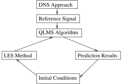
Initial Conditions DNS Approach
QLMS Algorithm Reference Signal
[image:4.612.332.541.53.198.2]LES Method Prediction Results
Fig. 1. The alternating process.
more effective and efficient method for wind profile prediction. In our current study, we mainly focus on the issue of efficiency, i.e. we aim to develop a method which can achieve a similar level of accuracy as the CFD approach but with a lower complexity. Certainly, it is possible to increase the complexity of the new method a little (but still lower than the original CFD approach) and achieve a more accurate result and in this case the new method could be more efficient and at the same time more effective as well.
In the combined method, the signal processing part employs the QLMS algorithm, while for the CFD part, LES based on the Smagorinsky SGS model will be employed. The alternating process is described as follows. First, the QLMS algorithm is used to obtain the predicted wind velocity, and then we use the prediction result as the initial conditions for the LES method for calculating the next stage of the wind velocity. In the next round, the same process is repeated. The process flow chart is shown in Fig. 1.
As the LES approach is accurate but time consuming with a high computational cost, and the QLMS algorithm has a very low complexity, an alternating combination of these two will produce a method with a much lower complexity.
NORMALISEDPREDICTIONERROR
P e1 e2
1 0.0538 0.0854 2 0.0969 0.0762 3 0.0889 0.0811 4 0.1115 0.0842 5 0.0880 0.0759
6 0.0861 0.0924 7 0.1042 0.1028 8 0.1013 0.0973 9 0.1022 0.0871
10 0.0960 0.0820
TABLE II RUNNINGTIME(SECONDS)
P t1 t2
1 260.9 214.1 2 484.6 380.4 3 832.2 533.2
4 1432.5 657.4 5 1813.6 787 6 1951.4 1015.9 7 2338.9 1253.2
8 2465 1177.1 9 2489.3 1464.7 10 3134.3 1646.4
sampling frequency with reasonable range of errors and use this sampling frequency to apply the QLMS algorithm and the CFD method for alternating prediction.
V. SIMULATION
Simulation results will be provided in this section to show the performance of the proposed alternating method. Based on an analysis of the correlation generated by the CFD data, we have chosen the sampling frequency as 1/6 Hz for this data set, i.e. the sampling interval between adjacent samples is 6 seconds. The other parameters are: the length of the FIR filter is L= 16and the step size isµ= 1×10⁻⁵
.
The results are shown in Table I, where the first column is the prediction advance value P, e1 the normalised error
between the LES method and the DNS method, ande2 is the
normalised error between the combined method and the DNS method. We can see that in terms of the normalised prediction error, the two methods have a very similar performance. As to the computational complexity, we show the running time of the two methods in Table II, wheret1 andt2 are for the LES
method and the alternating method, respectively. We can see that the running time for the LES method is nearly doubled when compared to the alternating method as the prediction advance step increases, highlighting the clear advantage of the proposed combined alternating method.
VI. CONCLUSIONS
In this work, both the CFD approach and the signal processing approach have been reviewed briefly, and a new
combined method is proposed by alternating the operation of the QLMS algorithm and the LES method one by one. As demonstrated by computer simulations, the proposed method has a much lower computational complexity with roughly half of the running time of a standard LES operation, while still maintaining a comparable performance in terms of prediction accuracy. In the future, a thorough study of this new method will be performed and its various extension/variation will also be investigated.
VII. ACKNOWLEDGEMENTS
This work is partially funded by National Grid UK and the National Natural Science Foundation of China (61628101).
REFERENCES
[1] N. Le Bihan and J. Mars, “Singular value decomposition of quaternion matrices: a new tool for vector-sensor signal processing,” Signal Pro-cessing, vol. 84, no. 7, pp. 1177–1199, 2004.
[2] X. Zhang, W. Liu, Y. Xu, and Z. Liu, “Quaternion-based worst case constrained beamformer based on electromagnetic vectoe-sensor arrays,” in Proc. IEEE International Conference on Acoustics, Speech, and Signal Processing, Vancouver, Canada, May 2013, pp. 4149–6153. [3] S. Pei and C. Cheng, “Color image processing by using binary
quaternion-moment-preserving thresholding technique,”IEEE Transac-tions on Image Processing, vol. 8, no. 5, pp. 614–628, 1999. [4] C. C. Took and D. P. Mandic, “The quaternion LMS algorithm for
adaptive filtering of hypercomplex processes,” IEEE Transactions on Signal Processing, vol. 57, no. 4, pp. 1316–1327, 2009.
[5] M. D. Jiang, W. Liu, Y. Li, and X. R. Zhang, “Frequency-domain quaternion-valued adaptive filtering and its application to wind profile prediction,” inProc. of the IEEE TENCON Conference, Xi’an, China, October 2013.
[6] M. D. Jiang, Y. Li, and W. Liu, “Properties of a general quaternion-valued gradient operator and its application to signal processing,”
Frontiers of Information Technology & Electronic Engineering, vol. 17, pp. 83–95, 2016.
[7] D. P. Mandic, C. Jahanchahi, and C. C. Took, “A quaternion gradient operator and its applications,”IEEE Signal Processing Letters, vol. 18, no. 1, pp. 47–50, 2011.
[8] D. H. Brandwood, “A complex gradient operator and its application in adaptive array theory,”IEE Proceedings H (Microwaves, Optics and Antennas), vol. 130, no. 1, pp. 11–16, 1983.
[9] W. Liu, “Antenna array signal processing for a quaternion-valued wireless communication system,” inThe Benjamin Franklin Symposium on Microwave and Antenna Sub-systems (BenMAS), Philadelphia, US, September 2014.
[10] ——, “Channel equalization and beamforming for quaternion-valued wireless communication systems,” Journal of the Franklin Institute, DOI: 10.1016/j.jfranklin.2016.10.043, 2016.
[11] S. Haykin,Adaptive Filter Theory, 3rd ed. Englewood Cliffs, New York: Prentice Hall, 1996.
[12] J. Ferzige and M. Peric,Computational methods for fluid dynamics. Springer, 2001.
[13] S. B. Pope,Turbulent flows. Cambridge university press, 2000. [14] S. Orszag, “Analytical theories of turbulence,”Journal of Fluid
Mechan-ics, vol. 41, no. 02, pp. 363–386, 1970.
[15] J. Smagorinsky, “General circulation experiments with the primitive equations: I. the basic experiment*,”Monthly weather review, vol. 91, no. 3, pp. 99–164, 1963.
[16] J. Deardorff, “A numerical study of three-dimensional turbulent channel flow at large reynolds numbers,”Journal of Fluid Mechanics, vol. 41, no. 02, pp. 453–480, 1970.