A STUDY OF A NEW
ELECTROMECHANICAL ENERGY CONVERSION PROCESS USING SUPERCONDUCTING FREQUENCY MODULATED RESONATORS
Thesis by Huan-chun Yen
In Partial Fulfillment of the Requirements for the Degree of
Doctor of Philosophy
California Institute of Technology Pasadena, California
1977
-iii-ACKNOWLEDGEt~ENT
I would like to express my sincere appreciation to the following persons who have made this work possible.
Professor J.E.Mercereau for his valuable advice, constructive criticism and continuous interest throughout this research,
Dr. G.J.Dick for his ingenious insight to this problem and many other things that he has taught me.
Dr. K.W.Shepard for his continuous interest, encouragement and help toward this research.
Dr. T.Yogi for his numerous personal advices and assistance in carrying out the experiment.
Dr. H.Notarys for his general help in the daily operation of the laboratory.
Mr. J.R.Delayen for his generosity of sharing his apparatus and data with me.
All the previous and present graduate student colleagues for making the laboratory also a pleasant place to work at nights.
~1r. S.Santantonio for his skillful machining of various reso-nators used for this study.
tvlr. E.P.Boud for his helpful and kind advice in addition to the technical assistance.
Ms. G.Kusudo for her enthusiastic administrative and general assistance for all my years as a graduate student.
-iv-Engineers, Inc, for the kind permission to reproduce the following figures;2.1, 2,9, 2,10, 3,1, 3,2, 3,3 which originally appeared in IEEE Trans MAG-11 and MAG-13.
The financial assistance throughout my graduate study is pro-vided by the California Institute of Technology and is greatly appreciated.
-v-ABSTRACT
Experimental demonstrations and theoretical analyses of a new electromechanical energy conversion process which is made feasible only
by the unique properties of superconductors are presented in this dissertation. This energy conversion process is characterized by a highly efficient direct energy transformation from microwave energy into mechanical energy or vice versa and can be achieved at high power level. It is an application of a well established physical principle known as the adiabatic theorem (Boltzmann-Ehrenfest theorem) and in this case time dependent superconducting boundaries provide the necessary interface between the microwave energy on one hand and the mechanical work on the other. The mechanism which brings about the conversion is another known phenomenon - the Doppler effect. The resonant frequency of a superconducting resonator undergoes continuous infinitesimal shifts when the resonator boundaries are adiabatically changed in time by an external mechanical mechanism. These small frequency shifts can accumulate coherently over an extended period of time to produce a macroscopic shift when the resonator remains
-vi-A highly reentrant superconducting resonator resonating in the range of 90 to 160 MHz was used for demonstrating this new conversion technique. The resonant frequency was mechanically modulated at a rate of two kilohertz. Experimental results showed that the time
evolution of the electromagnetic energy inside this frequency modulated (FM) superconducting resonator indeed behaved as predicted and thus demonstrated the unique features of this process. A proposed usage of FM superconducting resonators as electromechanical energy conversion devices is given along with some practical design considerations.
This device seems to be very promising in producing high power
(
~
lOW/cm3) microwave energy at 10 - 30 GHz.Weakly coupled FM resonator system is also analytically studied for its potential applications. This system shows an interesting switching characteristic with which the spatial distribution of micro-wave energies can be manipulated by external means. It was found that if the modulation was properly applied, a high degree (>95%) of uni-directional energy transfer from one resonator to the other could be accomplished. Applications of this characteristic to fabricate high efficiency energy switching devices and high power microwave
-vii-TABLE OF CONTENTS I. INTRODUCTION
References
II. FREQUENCY MODULATED (FM) SUPERCONDUCTING RESONATORS AND THEIR APPLICATIONS AS ELECTROMECHANICAL ENERGY CONVERSION DEVICES
1
6
7
2.1 Introduction 7
2.2 Adiabatic Principle (Boltzmann-Ehrenfest Theorem) 10 2.3 Experimental Studies of the New Electromechanical
Energy Conversion Scheme
2.3.1 Tunable Reentrant Resonator
2.3.2 Preparation of Superconducting Surface 2.3.3 Cryogenic Apparatus
2.3.4 RF Measurements
(a) Statically Tuned Resonators (b) Dynamically Modulated Resonators 2.3.5 Error Estimations
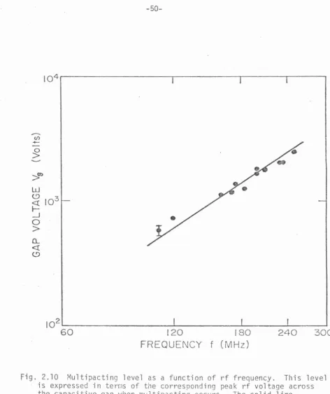
2.4 Results and Discussions
2.4.1 Static Electromagnetic Properties 2.4.2 Dynamic Electromagnetic Properties
(a) Typical Results 'tJith Small Frequency
16 17 25 27 29 29 34 45
46 46
51
Modulations 54
(b) Typical Results with Large Frequency
Modulations 63
2.5 Electromechanical Energy Conversion Devices Using
-viii-2.5,1 Brief Discussion of Conventional Electromecha-nical Devices for Energy Conversion 67 2,5.2 Characteristics of Electromechanical Energy
Conversion Devices Using Superconducting FM
Resonators 69
2,5,3 Some Design Considerations 79
2.6 Brief Comparison with Conventional Parametric Amp 1 ifi ers
2.7 Conclusions References
III, COUPLED FM RESONATOR SYSTEMS AND THEIR APPLICATIONS TO MICROWAVE ENERGY SWITCHING AND HIGH POWER MICROWAVE PULSE GENERATION
82
83
86
87
3.1 Introduction 87
3.2 Qualitative Analyses of Coupled Resonant Systems 87 3,3 Semiquantitative Study of Coupled Resonant System 104 3,4 Some Possible Applications Using Coupled
Super-conducting FM Resonator Systems 114
3.4.1 Characteristics of Energy Switching Devices 114 3.4.2 Characteristics of High Power Microwave
Generators 116
3.5 Conclusions References
Appendix A, AD I ABA TIC THEOREr1
Appendix B. A BRIEF DESCRIPTION OF THE ELECTROSTATIC TRANSDUCER
Appendix C. COUPLED MODE CALCULATION
117 119 120
_,_
Chapter I
INTRODUCTION
This thesis concerns a new process of energy conversion which is made feasible only by the unique properties of superconductors. The main thrust for this study is that with present-day superconduc-tivity technology, this application appears quite practical. In this dissertation we will not deal with the fundamental aspects of the superconductivity phenomena, instead, we will study the underlying principles for this application using our knowledge of superconductiv-ity and achievable technical expertise.
Superconductivity is a manifestation of a macroscopic coherent electronic state in certain metals, alloys and compounds when cooled below 23•K or so. It is characterized by the absence of d.c. electri-cal resistance (the perfect electrical conductivity) and by a perfect or near perfect diamagnetism (the Meissner effect). During the last three decades, a great deal of progress has been made both in under-standing the fundamental processes involved in the superconductivity and in advancing technologies for superconducting material processing. As a result, numerous practical applications based on these unique properties of superconductors have been proposed, demonstrated and realized, ranging from tiny quantum devices to huge superconducting magnet systems. Among these applications, the latter has been undoubt-edly the most successful application so far (1 ,2). Despite these notable achievements, almost all branches of applied superconductivity are still being actively pursued (3,4).
-2-identically zero for direct currents, It becomes finite however for time varying currents (a.c) even though it can remain quite
small up to frequencies in the infrared region. Physically this
finite a.c. loss can arise because of the inertia of the
super-conducting electrons inside the superconductor which prevents them
from responding to the external electric field instantaneously. The lagging in response results in incomplete screening of external
field which allows the field to penetrate into a thin layer (called
•
penetration depth, usually about several hundred A thick) on the
superconductor surface. The loss occurs when the normal electrons
which coexist with superconducting ones at finite temperature are driven by this residual field inside the penetration depth. However, this loss mechanism based on the superconducting-normal electron
model (two fluid model) is only a phenomenological account of the
possible mechanism. In 1957 Bardeen, Cooper and Schrieffer advanced
a microscopic theory of superconductivity based on quantum mechanics
(BCS theory) (5). There a new, dominant loss mechanism involving
the excitation of quasiparticles across a non-zero energy gap out of
the condenstate of a superconductor was proposed. Experimentally only part of the observed surface resistance can be explained in terms of this microscopic mechanism. The origin of the remaining part
-3-the surface resistance generally was also found to depend on the magnetic and/or electric field that the superconductor surface experienced (6,7,8,9).
Experimental studies at high field level have previously been associated with the effort to generate intense rf* fields inside superconducting resonators for charged particle accelerators. These studies have shown that the residual surface resistance Rs possibly
is due to dielectric loss on the surface, magnetic flux trapped inside superconductor, or acoustic phonon generation or any combination of them (6,7,8,9). Furthermore, these studies also showed that intense rf magnetic fields up tol600 gauss and rf electric fieldsup to 70 MV/m were obtainable inside microwave resonators, even exceeding the ther-modynamic values in some cases (6,10,11 ).
The implication of this spectacular reduction in rf surface resistance as well as the ability to support intense electromagnetic fields inside a resonator, is that superconductors can be used to fabricate devices and machinery operated at high rf power level. Such a development is now possible since the material technology for pro-ducing large high quality superconducting surfaces has become "routine" in many laboratories. This field is now known as "high power rf
superconductivity." Almost all previous high power rf applications have been centered around building superconducting particle
accelera-tors and related devices. Resonators of fixed resonant frequency
have been exclusively used in these applications and a good
-4-ing of their electromagnetic characteristics has been achieved. Proto-type superconducting accelerators are under development at several places both in the United States and abroad.
Tunable superconducting resonators whose resonant frequencies can
be continuously tuned or modulated on the other hand have not drawn
similar attention. The main reason seems to be lack of obvious
applications of frequency modulated (FM) resonators. There has been
a proposed application of FM resonator as an ultra sensitive
displace-ment transducer in the past (12). However the motivation behind the present work is to demonstrate the development of FM resonators as a new class of novel high power devices. In this dissertation,
ana-lytic and/or experimental foundations are laid illustrating the principle and its implementation via superconductivity as well as
some possible applications which are in turn evaluated with existing
superconductivity technologies. Among these applications are efficient electromechanical energy conversion devices; microwave energy switches and high power microwave pulse generators. Although basic physical concepts underlying these applications have been known for sometime and often appear in other contex~of physics, the subtleties of
applying these concepts in conjunction with extraordinary properties
of superconductors~to build useful devices and machinery are unique
and less familiar and will be explored in this dissertation.
The content of each chapter is outlined below: Chapter II deals with analytical and experimental studies on the properties of a
single FM resonator, using a highly reentrant resonator as an example.
present-
-5-ed along with some practical considerations. Chapter III discusses the behavior of a system composed of coupled FM resonators. The spatial and temporal energy distribution among the resonators are derived with the results applied to energy switching and pulse generation applicat-ions.
-6-References
1. V.L.Newhouse, Applied Superconductivity Vol. l
&
2. (AcademicPress, New York, 1975).
2. S.Foner and B.Schwartz, Superconducting Machines and Devices
(Plenum Press, New York, 1974).
3. 1974 Applied Superconductivity Conference, IEEE Trans. Mag. MAG-11,
95-883 (1975).
4. 1976 Applied Superconductivity Conference, IEEE Trans. Mag. MAG-13,
11-887 (1976).
5. J.Bardeen, L.N.Cooper and J.R.Schrieffer, Phys. Rev. 108,
1175-1204 (1957).
6. T.Yogi, Ph.D. Thesis, California Institute of Technology (1977).
7. J.Halbritter, IEEE Trans. Mag. MAG-11, 427-430 (1975).
8. J.M.Pierce, J. Appl. Phys. 44, 1342-1347 (1973).
9. J.R.Delayen, H.C.Yen, G.J.Dick, K.W.Shepard and J.E.Mercereau,
IEEE Trans. Mag. MAG-11, 408-410 (1975).
10. J.P.Turneaure and N.T.Viet, Appl. Phys. Lett.~. 333-335 (1970).
11. K.Schnitzke, H.Martens, B.Hillenbrand and H.Diepers, Phys. Lett.
45A, 241-242 (1973)
12. G.J.Dick and H.C.Yen, Proceedings of 1972 Applied Superconductivity
-7-Chapter II
FREQUENCY MODULATED (FM) SUPERCONDUCTING RESONATORS AND THEIR APPLICATIONS AS ELECTROMECHANICAL ENERGY CONVERSION DEVICES
2.1 Introduction
Resonators of fixed boundaries have been well studied in conven-tional microwave electronics. The resonant frequencies and correspond-ing mode configurations are determined by the resonator geometry and are mathematically obtained by solving Maxwell equations with appro-priate fixed boundary conditions. For an ideal resonator, a particular nondegenerate mode once excited will persist indefinitely in time. Since the resonator modes are standing wave modes, the electromagnetic energy associated with an excited mode is completely confined to
within the ideal conducting enclosure of the resonator. The fixed conducting boundaries of the resonator provide an isolating barrier across which no energy can flow into or out of the resonator.
-8-the resonator, mechanical energy can be exchanged with the
electro-magnetic energy via a moving boundary. This mode of energy exchange
is characterized by a direct conversion of low frequency mechanical
energy into high frequency electromagnetic energy or vice verse. The mechanism which brings about this energy conversion scheme
can be understood in terms of the familiar Doppler effect. To
illustrate this point, let us consider a specific example, namely an
ideal cylindrical resonator of radius Rand height h whose TE 111 mode is excited. The radius R is assumed to be fixed but the height can
be varied by making one end movable so that the resonator can be
tuned (modulated). This mode whose frequency depends only on the
position of the movable end for a given radius is characterized by
the absence of a longitudinal electric field along the axial direction of the cylinder. The longitudinal magnetic field has the usual
standing wave pattern which can be regarded as composed of two waves travelling oppositely to each other and being reflected at the two ends
of the cylinder. If the movable end is slowly moved inward, the reso-nant frequency f is increased. But each time the wave is reflected from the moving end, its frequency is Doppler shifted by a very small
amount. The shift is such that the new oscillation frequency matches the instantaneous resonant frequency to a high degree of accuracy. The mismatch
depends on the rate at which the end boundary is moved and can be made
-9-it nevertheless can accumulate from many reflections over a long
period of time to produce a macroscopic frequency change. Concurrent-ly with the frequency change, the time averaged electromagnetic energy associated with the oscillation inside the resonator is also changed by the same factor, because it can be shown quite generally the el
ec-tromagnetic energy is proportional to the oscillation frequency in
this ad1abatic limit (see further discussion in Sec. 2.2). The
increase in energy comes from the mechanical work done by the external modulation mechanism on the high frequency electromagnetic force
which is the counterpart of the Lorentz force at low frequencies
indicating the energy exchange with outside is now possible.
In order for the aforementioned accumulation to take place, we have tacitly assumed that the electromagnetic oscillation is sustained forever. This actually requires that two conditions be satisfied. The first condition which has already been assumed is that modulation must be done slowly so that over one period of the electromagnetic oscillation, the change in frequency is infinitesimally small. Under this adiabatic condition, the resonant oscillation will adjust to and follow the quasi-static change of the boundary. The second condition which bears directly to the usage of superconductors is that the electromagnetic energy inside the resonator should not decay
-10-of these two conditions are further discussed later in Sec.2.2, Sec. 2.4 and Sec. 2.5.
In this chapter, experimental evidence is presented to demonstrate the unique features of this new electromechanical energy conversion process using a superconducting resonator. The application of this scheme to fabricate practical devices is then discussed. The outline of each section is as follows: Section 2.2 reviews the fundamental
principle governing slowly frequency modulated resonators. Section
2.3 covers the experimental methods employed to study this conversion
scheme. Section 2.4 discusses the experimental results. Section 2.5
introduces an efficient electromechanical energy conversion device using an FM superconducting resonator as a component. The character-istics of this type device are then evaluated. A brief comparison with more familiar parametric amplifiers is also presented in Sec. 2.6.
2.2 Adiabatic Principle (Boltzmann-Ehrenfest Theorem)
The adiabatic principle is one of the important basic physical principles underlying this electromechanical energy conversion scheme. A general treatment leading to the Boltzmann formula and its
applicat-ion to an adiabatic transformatapplicat-ion resulting in adiabatic invariants of Ehrenfest has been given by L.Brillouin(l). Since we are interested in a system executing quasi-sinusoidal harmonic oscillation at
fre-quency f, the adiabatic principle will be reviewed here in terms of
harmonic oscillation parameters.
appli-
-11-cable to an adiabatically frequency modulated resonator, the results
obtained there are also applicable here. This is not completely
unexpected because after all the resonator is the counterpart of LC
resonant circuit at high frequency and quite often the essential
resonator characteristics can be obtained from its equivalent LC
circuit without the detailed knowledge of the field configurations.
In any case, the same results can br~ obtained from the first principle
with a given resonator geometry even though in reality this can be a
very complicated exercise. If we briefly summarized the results obtained
in Appendix A, the Boltzmann-Ehrenfest theorem can be stated as
follows: when a transformation is carried out on an ideal periodic
system of period T
= 1/f
by a very slow and continuous change of itsconstraint parameters, the product TW remains constant and constitutes
an adiabatic invariant of the transformation, where W is the total
energy of the system averaged over one period of oscillation.*
Mathe-matically, this theorem states that if the adiabatic condition
1
fTtT
df(t)
dt << f(t) ( 2. l )
is satisfied then for a dissipationless system the quantity W(t)/f111
is an adiabatic invariant. This comes about because as shown in
Appendix A,
* Strictly speaking, frequency is not defined for non-periodic osc~
-12-(2.2)
where
W(O),w(O)
ande
0 are respectively the initial energy, angular frequency and phase. s _
~
~~
is a dimensionless parameter charact-erizing the slowness of the adiabatic process. It can be seen from Eq.(2.1) that sis a very small number in the adiabatic limit. If we average Eq.(2.2) over one oscillating period, the right hand side of Eq.(2.2) becomes vanishingly small because the averaged trigonometric terms are essentially zero to a high degree of accuracy* (in addition to the smallness of s). Therefore we haveW(t) = constant f(t)
(2.3)
The bar indicates an averaging over one intrinsic oscillation period has been performed.
In this system, there are two scales of time variation that differ by several orders of magnitude from each other (adiabatic condition). The rapid time variation takes place approximately over the intrinsic oscillation period, in this example, the rf oscillation period. The slow time variation takes place approximately over the time scale during which the constraint parameters change significantly. The de-tailed electric and magnetic field distributions (or equivalently, the charge and current distributions) belong to the former and the total instantaneous energy, the oscillating frequency etc. belong to the
-13-latter category.*
Equation (2.1) shows that the theorem requires the frequency
change during one period of oscillation be infinitesimally small
compared to the frequency itself. In general a quantity A(t) is said to be adiabatically varied if it satisfies the following relationship:
1 dA(t)
f(t) dt
« A(t) (2.4)
A dimensionless parameter sA as defined by Eq(2.5) can then be used to measure the slowness of the changing in A(t).
(2.5)
If A(t) is the instantaneous angular frequency, we have for a
mecha-nically modulated microwave resonator at 1 GHz
s w 'V _ ____,1 _ _ ~ --....!,-=--~- 'V 1 0-6
w(t)·,m 21T·l09·10-4
(2.6)
where ' m is the characteristic mechanical modulation time- The value -4
of 10 sec for ' m is considered as near the upper limit achievable
with present rotating machines. This shows s is indeed a very small
w
number as assumed before. Thus when an adiabatically varying quantity
A(t) can be expanded into an ascending power series in sA, second or
*Since quantities that vary appreciably only over many rf oscillating periods are of main interest, let it be understood that whenever they are expressed in the form A(t), an average over one rf period is
assumed unless otherwise stated. In that limit, they can be considered as the instantaneous values. Hereafter the bar over an averaged
-14-higher order terms can be completely neglected. Quite often even the
first order terms are negligible too, This gives us some insights into
the nature of the adiabatic invariant. An invariant strictly speaking
is not a constant,rather its difference from a constant value can be
made as small as we wish and for practical purpose can be treated
as a constant.
If dissipations are present in the quasiperiodic system, adiabatic
invariants no longer exist. In Appendix A, it is shown that in the
presence of dissipation, Eq.(2.3) is replaced by Eq. (2.7).
W(t) _
(t
dtf(t) - constant·exp{ -
1
0 'p(t) ) (2. 7)where 'p(t) is the instantaneous energy decay time which can depend on
the frequency and therefore the time. The exponent of Eq.(2.7) shows
the integral effect of all the losses up to the time t when started
with a fixed amount of energy at t = 0.
Take time derivative of Eq.(2.7) we obtain
~=W(-1-ut 'm
( d ) -1
where 'm
=
dt lnf_1 )
'p
( 2. 8)
is previously identified as the characteristic
modulation time. Clearly if the dissipation is so excessive that
Tp « Tm' the system behavior is dominated by the irreversible decaying
process without noticeable modulation effect at all. On the other
hand, if the energy does not dissipate significantly (such as the case
with a superconducting resonator) so that TP >> Tm the system is
prac-tically dominated by the modulation effect. As noted before, in the
-15-and energy to change gradually as a result of continuous Doppler's shift
upon reflecting from a moving boundary many times. As for the moving
boundary, the modulation causes it to experience a continuous net momentum and energy transfer across the boundary because both the
total energy and momenta are conserved for the whole system (electro-magnetic fields, resonator and modulation source). The net momentum transfer across the boundary results in a pressure exerted upon it, while the net energy transfer results in the energy conversion between
electromagnetic and mechanical forms. This conversion process based
upon Doppler effect is intrinsically highly efficient and if done adiabatically is also reversible. The reason is that the interplay of
the energy conversion is purely electromechanical in nature rather than
thermodynamical, therefore ordinary thermodynamic limitation does not apply here. If we bonow the concept of "entropy" from thermodynamics, this process can be viewed from a different angle. The state when an
ideal fixed resonator is at resonance is no doubt a very special state of the system (the familiar notion of eigenstate). In order for an
oscillation to sustain itself indefinitely, the phase change over an
"oscillating path" has to be exactly a multiple of 2'1T. In a way,the state
meeting this requirement represents a highly "ordered" state with a
minimal "entropy". When the boundary is adiabatically modulated, the
oscillation inside is sustained and made to follow external modulation. The phase relationship is preserved through continuous change in fre-quency. Thus for this process, the system remains highly "ordered"
and the system "entropy" is unchanged. Furthermore, the slowness is
-16-modulation can cause sufficiently large phase change so that the
instantaneous state of the oscillation depends very critically on the
detail nature of the modulation. It is interesting to note that the
requirement of reversibility and its consequence of no increase in
"entropy" are the same for a reversible thermodynamic process.
How-ever, the similarity ends here. For an electromechanical conversion
there is no fundamental limitation on how much mechanical energy r.an
be converted i~to electromagnetic energy through modulations or vice
versa; while for a thermodynamic conversion it is limited by the
tem-perature of the two thermal baths which are employed in the process
in a very fundamental way. The reason that the temperature plays
such an important role in the thermodynamic conversion is that the
mechanical work available is extracted from the internal energy of
the working medium used in the conversion process. Microscopically
the internal energy comes from the highly incoherent thermal energies
associated with the internal degrees of freedom. Temperature is merely
a macroscopic parameter used to characterize this internal energy.
Thus the thermodynamic conversion actually converts a highly incoherent
internal energy into a highly coherent mechanical energy. On the
contrary, our electromechanical conversion converts an already coherent
oscillation energy into another coherent form (mechanical energy) or
vice versa.
2.3 Experimental Studies of the New Electromechanical Energy Conversion
Scheme.
A highly reentrant superconducting resonator was used to study
-17-the static electromagnetic properties of this resonator have been
studied in great detail, the results will be concisely presented only
to the extent which is useful for our purpose of demonstrating this conversion technique.* The dynamic electromagnetic properties are
then presented to show the time dependent behavior of the stored
electromagnetic energy inside the resonator as a result of the electro-mechanical energy conversion.
2.3.1 Tunable Reentrant Resonator
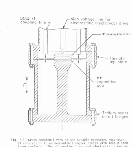
Cross sectional view of the reentrant resonator used in this
study is shown in Fig. 2.1. The resonator consists of three demountable pieces -- a circular base with a post located at the center, a
cylin-drical housing and a thin top plate. They were machined out of oxygen
free high conductivity copper (OFHC) for easy lead electroplating and
assembly. Indium gaskets were exclusively used for vacuum seals as
well as rf current carrying joints.
The electromagnetic properties of this reentrant cavity were
evaluated in terms of a lumped parameter model consisting of a tance terminated coaxial transmission line. Because of strong
capaci-tive loading of this reentrant design, the resonant frequency was de-termined to a large extent by the size of the capacitive gap between
the top plate and the central pole.
The thickness of the top plate was reduced to 50 mils in an
annular region as shown in Fig.2,1 in order to maximize the mechanical compliance of this element. The minimum thickness was determined by
the necessity of conducting the heat generated by rf losses in the rf
50.0.
rf coupling
-18-high voltage line for
electrostatic mechanical drive
- - T r a n s d u c e r
flexible
top plate
rf
capacitive gap
Indium sea Is on all flanges
Fig. 2.1 Cross sectional view of the tunable reentrant resonator.
It consists of three demountable copper pieces with lead-plated
inner surfaces. The rf coupling lines and electrostatic mecha
[image:26.569.43.503.75.582.2]
-19-capacitive region to the external helium bath. The present design
provides a thermal conductivity of about one watt per •K temperature
rise in the center of the top plate and a mechanical compliance of
2.5xl06 newton/m.
Frequency tuning of the resonator was accomplished by changing
the rf gap size through mechanical deformation of the top plate both
statically and dynamically. For the former, the top plate was
static-ally loaded through a mechanical linkage causing it to deflect with an
amplitude of a few mils which corresponds to a frequency range of 80
to 300 MHz. Any frequency within that range could be obtained
reproduc-ibly to within 20 KHz. All the static frequency dependent
electro-magnetic properties were studies with this method.
For dynamic tuning, the fundamental mechanical mode (drumhead
mode) of the top plate was excited by an electrostatic transducer as
shown in Fig.2.1.* The plate was excited to vibrate with a few mil
amplitude by an alternating voltage of a few kilovolts at the frequency
of its fundamental mode (about two kilohertz). Thus the cavity could
be frequency modulated rapidly at the rate of about 1012 Hz/sec. The
time dependent electromagnetic properties and electromechanical energy
conversion were studied with this method.
In order to understand the experimental results, the relationship
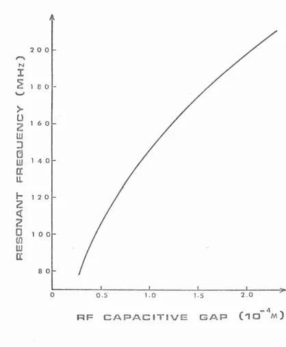
between ·the rf capacitive gap size and the resonant frequency is
need-ed. This was found experimentally by putting various circular brass
shims of known thickness between the top plate and the cylindrical
-20-housing so that the gap size d could be known before the resonant frequency f was measured. The functional relationship between f and
d was then found by fitting experimental data pairs (f,d) with the
best fitting given by
1 = 0.4357 + 0.037
f2
a
(2.9)h -4
w ere f is in 100 MHz and d in 10 m. Eq.(2.9) is plotted in Fig.2.2. Because the geometry of our cavity is much smaller than the free space wavelength at the resonant frequency, lumped parameter
approximation consisting of an equivalent inductance L and a
capaci-tance C is expected to be sufficient for most first order calculations.
The equivalent inductance L is equal to the total inductance of the
coaxial section and does not change with the frequency. Its value was calculated from the geometry of the coaxial section and found to
-8
be 2.62 x 10 h. The equivalent capacitance C consists of two parts
c
1 andc
2:c
1 comes from the capacitance of the coaxial section andis a constant (about 3.43 pf), while
c
2 comes from the ''parallel plate capacitance'' of the gap region and is time dependent. Over thefrequency range of interest,
c
2 becomes the dominant part withc
1accounting for only 4% to 8% of the total equivalent capacitance.
From the known equivalent inductance L and capacitance C, the
resonant frequency was found by the usual relationship (2nf)2 =
~C'
and was given by1 = 0.436 + 0.0355 (2.10)
~
d~
N
:I
~
""""
>
u
2
w
:J
l'J
w
a
LL
...
2
~2
0
Ul
w
a
-21-200
1 8 0
1 2 0
0 o.s 1.0
RF CAPACITIVE
l-5
GAP
(10 -4 ) MFig. 2.2 Best fit of t~e experimentally determined resonant frequency
[image:29.567.81.499.69.576.2]
-22-compares very favorably with Eq.{2.9), indicating lumped parameter
approximation is indeed adequate.
The field distributions in the resonator are characterized by a highly concentrated axial electric field in the gap region and a
vanishingly small radial electric field in regions far from it. A
schematic diagram showing the field lines of the fundamental mode is
given in Fig.2.3. The magnetic field was deliberately made small
everywhere inside the resonator because the resonator was originally
designed to study the electrical properties of lead surface,therefore
magnetic field was minimized to suppress its effects. It turns out
this arrangement is also suitable for our present purpose. Not only
is large frequency modulation easily achieved, but the modulation
process is simple enough to make model calculation possible as
illus-trated below.
The energy content W(t) inside the resonator at any instant t
is given by
(2.11)
where the integral is carried out over the resonator volume at that
instant. E{r,t)* and H{r,t) are respectively the instantaneous
elec-tric and magnetic field inside. £ and ~ are respectively the
permit-tivity and the permeability of the volume V. The energy change in
W(t) can be realized by changing the field strengths as well as the
-23
-•
•
•
•
•
•
•
•
•
ELECTRIC FIELD LINE
e MAGNETIC FIELD LINE
Fig. 2.3 Schematic drawing of the field profiles of the fundamental
resonant ~ode. It shows a large axial electric field concentrated
in the rf gap region and generally weak field elsewhere. The gap
[image:31.571.154.450.95.526.2]
-24-in the adiabatic limit, the volume change is extremely small over one intrinsic oscillation period (refer to previous discussion in Sec. 2.1 and 2.2). If we average Eq.(2.ll) over one rf period, and take into account the fact the contribution from either term is almost identical*, we have
W(t) =
r
~ Eo
2c~,t)dV
(2.12))vol
where our averaging convention has been used. It should be pointed out that all the time variations in Eq.(2. 12) which include the chang-ing in the field amplitude and volume are now on a much slower scale. If we define an 11instantaneous" effective volume Veff so that
(2.13)
where Epk(t) is the uniform peak electric field across the parallel
plate gap region. As noted before, since the electric field is highly concentrated in the gap region for this resonator, the effective
volume Veff is expected to be roughly equal to the instantaneous gap volume (refer to Fig. 2.1).
Equation (2.13) is in consistency with the lumped parameter approximation because under the same conditions, the energy is given by
W(t) = }
C(t)V~(t)
( 2.14)
-25-where C(t) is the instantaneous equivalent capacitance, and Vg(t) is the peak voltage across the gap.
Since the field is quite uniform in the gap region, Eq.(2.14) can be further written as
=
l (
1 + Cl ) ·c
2(t) ·d2(t)Ep2k(t)2 C2(t) (2.15)
(2.16)
where A is the area of the parallel plate and Vgap is the gap volume
enclosed by the area A and height d(t). Compared with Eq.(2.13) we
get
cl
veff = vgap(l +c
2(t))
(2. 17)
cl
Because the factor (1 +
c-{t))
varies from 1.042 to 1.087 in this2
study, using a constant of value of 1.065 only incurs an error of less
than 2.2% in the energy over the entire range. Later we will use these
results for data analysis.
2.3.2 Preparation of Superconducting Surface
After the required parts were machined out of OFHC copper, they
-26-then with levigated alumina polishing compound (grain size 1~3 ~). Subsequent lead electroplating essentially followed the standard in-dustrial procedures* with minor modifications. Since detailed inform-mation is available elsewhere (3), only a brief description is given below:
(1) Cleaning: After mechanical polishing, organic material was removed with organic solvents such as acetor.e and trichloroethylene. The
copper surface was then electropolished in a phosphoric acid bath** with a lead cathode to remove among other things the copper oxide, (2) Electroplating: Immediately after electropolishing, the solution was rinsed away and the work piece was placed in a lead fluoroborate bath*** with lead electrodes made out of 99.9% purity lead foil.
Initially a few short D.C. pulses (~1 sec) were applied at a current density of 80 A/cm2 to insure a complete coverage. Subsequently plating was continued at reduced current density of 8 mA/cm2 until desired thickness was obtained.
(3) Chemical polishing: After plating, work piece was rinsed with
deionized water before being chemically polished with an acid mix-ture**** and chelated with diluted EDTA.
(4) Drying: The surface was then treated with 7,5% ammonia and rinsed with acetone before being blown dry with dry nitrogen gas.
* Electroplating Engineering Handbook. ed. by A. Kenneth Graham
(Reinhold Publishing Corporation).
**The electropolishing solution is a mixture of one part Electro-Glo "200" (Electro-Glo Co. Chicago) and three parts 85% phosphoric acid by volume.
***One part "Shinol LF-3" (Harstan Chemical Company Brooklyn, N.Y.), 23 parts of 50% lead fluoborate and 26 parts of H~O by volume.
-27-(5) Preserving: Before the resonator was assembled, the plated pieces
were kept in vacuum or inside a pressured chamber filled with dry
nitrogen gas to preserve the fresh lead surface.
The properties of superconducting lead surface obtained in this
method have been published and can be found elsewhere (2).
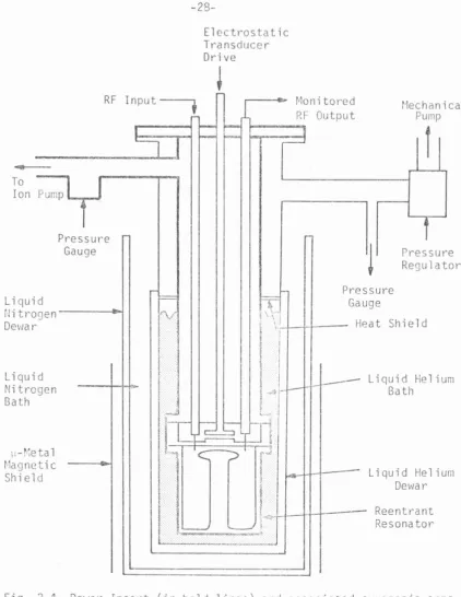
2.3.3 Cryogenic Apparatus
After electroplating, the resonator was assembled before it
was attached to the bottom of a dewar insert and pumped down to a
-5
pressure of 10 Torr or lower to prevent further surface deterioration.
Indium gaskets were used for vacuum seals. A schematic diagram of
the dewar, the insert and their accessories is shown in Fig.2.4.
The insert consisted mainly of three verticle probes: two
were SOn coaxial lines for rf circuits; the third was used either as
a high voltage line or a mechanical linkage. For low temperature
experiments, a 4 inch stainless steel dewar was used along with
stand-ard cryogenic equipment as shown. Ambient earth magnetic field was
reduced with a mu-metal shield to below 15 milligauss over the
exper-imental region. The temperature of the helium bath was varied by
pumping on its vapor in conjunction with a pressure regulation system.
The temperature was determined by monitoring the equilibrium vapor
pressure by a Wallace and Trernan pressure gauge, and converting by
the 1958 He4 scale of temperature. Typical temperature variation
covered in the experiments ranged from 4.2 •K to 2 °K. During the
(continued from previous page)
****
One part of glacial acetic acid, 2 parts of6 parts of 30% H/02, 9 parts of saturated EDTA,
H
2
o,
all by volume.70% nitric acid,
-28-Electrostatic Transducer Drive
•
RF Input
---,f
1 ~1oni to red
,1. RF Output
tlechan i cal Pump
•
ToIon Pump( J
1
PressureGauge
Liquid
!litro~en---l~oi De\-Jar
...-l--~ ~ - ~----... J
I
~- r---~l
i
Pressure Gauge
f
i
Pressure RegulatorHeat Shield
Liquid Nitrogen Bath
- - + - I H •
f.J-
~
~r--1 ----Liquid Helium Bath1 -~~eta 1
nagnetic
Shield
h-
L
.
l
l
'~
i
·~
'c....
;:>r
I
I
I
1,h
'==="'---
'
L.r-...4-+--t---- L i qui d He 1 i um
De\-Ja r
~~--~+--- Reentrant
Resonator
Fig. 2.4 Dewar Insert (in bold lines) and associated cyrogenic appa -ratus used in this study. Non1a ll y the resonator was operated at 4.2 K. For lm.ver-temperature operation, a r1echanical pump was used to pump on the helium vapor in connection with a pressure
[image:36.572.79.501.53.599.2]
-29-experiments, the pressure inside the resonator was maintained below -7
10 Torr with a differential ion pump.
2.3.4 RF Measurements
Standard rf instrumentation was used for all the experiments. To insure proper impedance matching, all the electronics including coaxial lines were made to have characteristic impedance of 50n. For a study of the static frequency dependent properties, the technique followed standard procedures for exciting a superconducting resonator of fixed resonant frequency discussed below in subsection (a). For the study of the time dependent properties, an electronic scheme was designed to inject and monitor the time dependent rf energy inside the resonator as discussed below in subsection (b).
(a) Statically tuned resonators:
When the resonator was statically tuned, rf excitation was accomplished by one of the following methods; namely the phase-locked loop or a self-oscillation loop. The block diagrams showing the elec-tronic components and arrangements for both methods are given in Figs,2.5 and 2.6 respectively. Since the detailed theory of the loop operations and measurement techniques are discussed extensively in the literature (4), only a simplified theory of operation relating the measured quantities to the properties of the resonator is given here. Our notations will follow those in (5).
MODULATION.---, R F OUTPUT PULS E GENE RA TOR TRIG . INPUT RF OUTPUT F RE Q U E N -VOLTA GE CO N TRO L L E D OSCl LLATOR FREQ UENCY CONT R OL INPUT DC AM PLIFI E R CY I ~ ~ COUN TE R
0
OSClL LO-~ SCO P E R F voLT M E Te R
I
1
P HAS E 0 R 1 S HIFTER POW E R METE R-{
~;
E
~
PPU 'I>P
INC D lR ECTIONAl COUPLER1---~>
PREF RE SON AT O R ~ '--. . ,. PO WER D IVI D E R Fig. 2 . 5 B l ock diagram of a phase -locked loop for exc i tinQ a highQ
resonator of fixed resona n t frequenciesPULSE
GENERATOR
0
OSCILLO- SCOPE
RF
VOLTMETER OR
POWER METER PIN C PRE F PPU MIXER PREAMP POWER A MP LIFIER
VARIABLE ATTENUATOR
(CWMODEJ
AMPLITUDE Ll
MITER
FREQUENCY COUNTER
PHASE SHIFTER
'-1
~
P,NC O I Rt:CTIONAL COUPLER ,..._,___
_
... PREFPOWER DIVIDER
RESONATOR PPU Fig. 2.6 Block diagram of a self-oscillation loop for exciting a high
Q
resonator of fixed resonant frequencies.
-32-measured quantities were the unloaded power decay time Tpo• the
incident power Pine' the reflected power Pref and the monitored signal
Ppu (refer to Figs.2.4 and 2.5 for definitions of these quantities).
Conservation of energy requires
(2.18)
where Pdiss is the power dissipated in the resonator itself, dW
dt is
the time rate of change of the field energy stored inside the resonator.
For a fixed coupling, the monitored signal P is proportional
pu to the energy content W(t}, i.e.,
(2.19)
From the definition of the unloaded quality factor Q
0
Q
=
w~l =0 p-d. WTpO
lSS
(2.20)
we get
P. - p 1 d
1 nc ref _ 1 _ _ ~ 1 n P ) )
Ppu k dt pu ( 2. 21 )
Once the proportional constant k (coupling parameter) is known, the
energy content, and therefore the rf voltage across the capacitive
gap at steady state can be determined by the measured quantity Ppu as
indicated by Eqs. (2.10) and (2.14).
Experimentally, two methods were available for determining the
-33-Method I. At steady state, with incident rf energy probe critically
d
coupled to the resonator (i.e., when
df
= 0 and Pref = 0), we haveP. lnC
=
Pd. lSS + ppu (2.22)Since the monitoring probe was extremely weakly coupled to the
resonator
therefore
and
i.e.,
and
p pu « pd1 . ss
Pine "' Pdiss
w
"' P. 1nck =
~=
w
=
wW pdissTpo
PEU ·p T po inc
Thus by measuring Pine' Ppu' Tpo' one can determinek.
~1ethod I I
(2.23)
(2.24)
From Eq.(2.14) the energy content of the resonator is equal to
w
=l
cv
22 g
where C is the equivalent capacitance and Vg is the peak voltage
across the capacitive gap. Suppose an rf voltage is directly applied
-34-small hole in the center of the top plate. If the resonator is assumed to be an ideal open circuit at resonance, then the incident voltage V+ and the reflected voltage V at the resonator are related to the voltage across the gap V by the g following equation:
=
v
/2g (2.25)
Experimentally what was measured were the incident and reflected voltages at the respective ports of a directional coupler: V~ and V'. After taking into account the attenuation properly, we can relate
(V~, V~) to (V+' V_) with two attenuation coefficients a and 8 so that
V' = aV
+ +
(2.26)
V'
:;:;
f3VEquation (2.25) can be written as
V g :;:;
2~V
+ V _ :;:; 2j a f3 (2. 27)that is, Vg is determined by the measured V~, V~, a and f3.
The coupling parameter k is finally obtained as follows:
(2.28)
At a particular frequency, Ppu is measured for a given Vg and apply Eq.(2.28) to obtain the value of k.
(b) Dynamically modulated resonators
-35-described schemes for exciting the resonator become impractical because the resonant frequency is continuously changing rapidly in time. Our usual understanding of microwave resonator systems derived from solving Maxwell's equations with appropriate fixed boundary conditions can no longer directly apply. With boundaries constantly changing, the problem generally becomes not so well defined and harder to handle. However, in the limit of very slow change (adiabatic limit), the bound-aries can be regarded as quasi-static and the corresponding instanta-neous boundary value problem can be solved. The solution so obtained is assumed to approach the real situation in the slow limit.
Experimentally, an electronic scheme whose block diagram is shown in Fig. 2.7 was used to accomplish the excitation of the resonator. The thin top plate was driven to vibrate at its fundamental mechanical mode at a rate of about two kilohertz. The corresponding rf resonant frequency could ~hus be modulated over a wide range (up to a factor of two in resonant frequency) in the region of one to two hundred
megahertz. RF pulses of various durations ranging from 5 to 20 ~s were injected into the resonator through the incident probe at a specific point of the mechanical cycle when the frequency of the incident rf pulse matched the instantaneous resonant frequency. It was found pulses with width less than 5~s coupled poorly to the resonator. It is believed to be due to insufficient coupling to build up a noticeable amplitude. This is plausible because the typical voltage decay time
R F OSCILLATOR
@IXE:
"'
""
PULSE-v
.
v
'
GENERATOR .. P,NC TRIG .i
PULSE D :RE CTIONAL I SHAPI N G HI-VOL TA GE ~ COU P LER A T RANS u UCER DELAYED GAJ.! V ARIAB LE D R IVE --. PREF f ~....
DeLAY TRIG ....
~ ~ · r -I TR A NS-,..._0
V O LTAGE .A DUGR...
RESONA TOR...
...
....
D iVIDER SOQ 20 DB~
OSCIL LO-RF VOL T METE R P R~C ISIO N --.A ATT ENUATORPpu
SCO P E...
~ -v . '. P OWER METE R F ig . 2,7 B l ock d i ag ra m of t h e electro n ic sc h eme f or in jec t ing rf energy pu l ses in to a hi gh l y f requency mo d u l ated superconducting resonator . To coord i na t e the i nj ec tion and the p l ate vibrat i on , a sig n al derived f r an the transducer dr i v e was p h ase shifted before being used to trigger a pu l se generator which i n tu r n gated the rf energy,I w
-37-which is obtained when the resonator is driven by a CW source of the same strength. Furthermore, within 5 ~s, the resonator frequency
changes by about 1 MHz which which may be sufficient to cause some fre~uency
mismatch between the input and the resonator. Therefore the effective pulse duration is much less than 5 ~s, and the oscillation amplitude is further reduced.
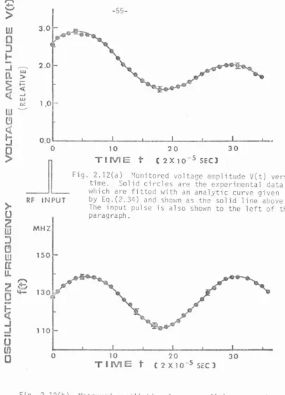
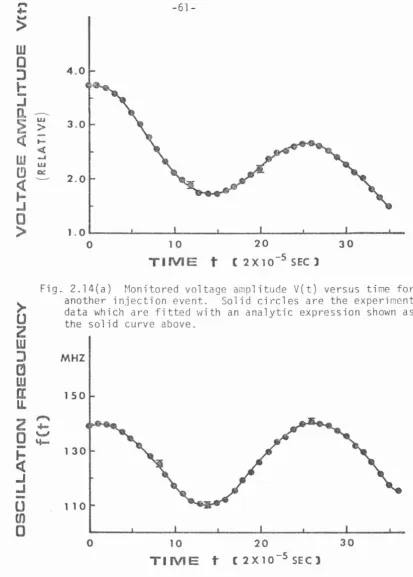
After injection, rf input ceased and the subsequent time evo-lution of the stored electromagnetic energy inside the FM resonator was monitored through another probe weakly coupled to the resonator. The monitored signal was then fed into a calibrated rf voltage
measuring device for amplitude measurement. The corresponding instan-taneous frequency was determined by beating this signal with a local oscillator (detailed information given below). To coordinate the rf energy injection and the plate vibration, an attenuated signal from the transducer drive was fed into a variable phase shifter. The
phase shifted signal triggered a pulse generator which in turn gated the rf energy. The amount of delay was adjusted manually to achieve resonance. The interval between injections was made to be longer than the power decay time, so that the observed signal was due to one event only. The scheme was also modified so that multiple pulses of different frequencies could be injected into the resonator at different mechanical phase points to examine their possible inter-action,
-38-quantities (V(t), f(t)), where V(t) is the monitored voltage amplitude*,
and f(t) is the instantaneous frequency. Operationally the voltage
observed through the monitoring probe was first fed into a terminated
rf voltage measuring system which had a bandwidth of at least 400 MHz
(the frequency of the modulated signal ranges from 95 MHz to 155 MHz
in this study). This terminated signal was displayed on a Tektronix
scope which had a bandwidth of about 150 MHz. For each rf energy
pulse injected, the corresponding evolution of the stored energy was
displayed on the scope. A polaroid picture of this trace was taken
for amplitude measurement later. A typical trace is shown in Fig. 2.11.
The amplitude measured from the expanded polaroid picture at any time
was corrected for any possible frequency dependence of the voltage
measurement system. This was done by feeding a calibrated rf signal
from a Hewlett-Packard 608F signal generator into the voltage
measure-ment system to produce the same amplitude at the same frequency on
the scope (frequency determination is discussed below). The calibrated
output of the oscillator was then read from an rf voltmeter. For
frequency measurement, the same monitored voltage V(t) was beat with
a local oscillator first before being displayed on the scope. Marks
showing the zero beat were used for frequency identification at these
instants. Because of finite time resolution on the scope screen as
well as finite width of zero beat mark, the frequency so determined
was an averaged frequency over at least two hundred rf cycles. The
-
39-amplitude measurement described above was carried out for each instant
where the frequency was also known.
Before proceeding to discuss the evolution of the stored energy,
the nature of our measured quantities V(t) and f(t) should be carefully
examined. This was necessary because on one hand the measurements
made actually represented information of what had already taken place
a while ago (typically 6 ns) at the resonator site. On the other
hand, the voltage V(t) contained frequency components that were
dis-tributed over a wide spectrum. For the voltage V(t) to represent
truthfully the history of the stored energy inside the resonator, the
time delay between the observation and actual event must be the same
for each frequency component, that is, the propagation medium in
between must be non-dispersive. Generally speaking, a signal
contain-ing a wide range of frequency components can be distorted by the
dispersion as well as the attenuation of the propagation medium.
The attenuation aspect (frequency response) can be corrected with a
calibrated source as explained above for the amplitude correction.
The dispersion effect however is much harder to eliminate unless a
non-dispersive medium can be found. An experiment was done to check
the dispersion properties of our measuring system. Signals from a
generator were fed directly into the measuring system, the resultant
time delay was measured for each frequency. It was found the delays
were within 4ns of each other for all frequencies of interest. This
small amount of difference in delay time causes no actual difficulty
-40-change is on the time scale of the mechanical period which is about
500 ~s. and the time resolution of each voltage amplitude measurement
from the polaroid picture is about 2 ~s during which the frequency
change is much less than 1 MHz. Obviously the voltage so measured
was an averaged value over several hundred rf cycles too.
There was another subtle point which had to be clarified before
the measured values could be used without ambiguity. As noted before
the voltage measurement and the frequency measurement were separately
carried out with the same monitored signal but slightly different
electronic circuits. The time delay between these two different
circuitry paths must be small enough so that it is legitimate to
correlate the frequency measurement to voltage measurement at
appar-ently the same point. Even though experimental deter~ination of this
relative delay was done with somewhat large uncertainty due to the
difficulty of comparing two quite different signals, it is
neverthe-less conservatively estimated to be no more than several ns by
con-sidering the behavior of the mixer used here for the frequency mixing.
With 2-3 ~s time resolution for actual measurement, this kind of delay
was completely buried inside the measurement error itself and causes
no additional uncertainty and ambiguity.
In order to study the time behavior of the stored energy W(t),
the relationship between the corrected voltage V(t) and W(t) has to
be known. Since the monitoring line was extremely weakly capacitively
coupled to the resonator before the top plate was induced to vibrate,
it was expected that the coupling would remain very weak for a not too
-41-A separate calibration was done to determine this frequency dependence. During the calibration the monitoring probe was clamped to a fixed position and was weakly coupled to the resonator. The resonant frequency was then changed by statically deforming the top plate*. For each frequency, the resonator was critically driven so that the peak voltage across the gap Vg was known (see subsection (a)). Plot-ting the ratio of the monitored vo1tage V(t) to Vg versus the fre-quency, a linear relationship was found from 100 MHz to 175 MHz,
indicating a lumped circuit approximation (see Fig. 2.8) with a constant coupling capacitance was adequate as elaborated further below.
In this lumped circuit approximation, the voltage amplitude V(t) and the peak voltage across the gap Vg are related by the follow-ing equations
(2.29)
where V1(t) and
v
2(t) are respectively the instantaneous voltages across the variable capacitor C and the termination resistor Rand are defined by the following equation*
v
1 ( t) -V (t)sin(ft
wdt + el )g 0
v
2(t) -V
(t)sin(~:
w
dt
+e2)
L
-42-FM
RESONATOR
Co
c
v
1 ( t) = V2(t) i RCo 1 ft -ooV2(t)dtwhere
v
1(t) - V (t)sin(ft wdt + e1)g 0
t
V2(t) - V ( t ) S i n
1
0
c.ud t + 0 2 )
R
50!}
Fig. 2.8 The equivalent circuit showing the relationship between the
instantaneous voltage across the rf capacitive gap V (t) to that
a~ross
thet~r
mination
resistor V?.(t) .. Vg(t) and V(t) are respec [image:50.572.117.420.106.459.2]
-43-where
e
1 ande
2 are the initial phases,Thus if V(t) is known, Vg(t) and therefore W(t) can then be obtained from Eqs,(2,29) and (2,14). The calibration asserted that the coupling capacitance C
0 is essentially constant. This is made clearer if we take liberty of Fourier analysis and treat the circuit as if it were time independent, then V and Vg are related by
(2.30)
Since monitoring line was weakly coupled to the resonator, C0 was found to be much less than 1 pf.* With R =
so
n
,
wRC0
~
10-3
~
10-4 Eq.(2.30) can be approximately written as
(2.31)
which is consistent with the calibration result.
It should be pointed out though that it is not immediately clear that Eq.(2.30) is also valid for a frequency modulated voltage source Vg. In any case, Eq.(2.29) is the fundamental equation relating Vg and V. It will be shown next that in the adiabatic limit, Eq.(2.31)
is the zeroth order solution of Eq.(2.29).
Because Eq.(2.29) involves quantities which vary either rapidly or slowiy in time, it is awkward to deal with them simultaneously. Since we are more interested in the slowly varying quantities, we
*Perform one static measurement and with known values of
v
9, V, w and R, C
-44-shall set up equations which contain them only.
Define
X
=J:
wdt +e
1n = 82 - 8
1
Differentiate Eq.(2.29) and equate the coefficients of sinx and cosx
terms on both sides we obtain the desired set of equations
dV dV V
CJf
= - wVs inn + ( dt + RC ) cos n0
dV V wV
9 = wVcosn + (dt + RC ) sin n 0
Eliminating n from these two equations, we have
Since
~
"'
~
«wV dt Tt'fl 9
dV
"'
v
<< wV <<dt fin
therefore (wV ) 2 "'
(
_
v
_
)2g
RC
0
i.e.
lvl "'
wc Rlv
I
0 y
which is identical to Eq.{2.3l).
v
RC
0 { ·: wRC « 1)
-45-Finally the stored energy is related to the measured quantities V(t), f(t) as follows:
W(t) =
~
C(t)V~(t)
1
v
2(t) (2.32)=
2L(41T 2
c
R)20 f 4 (t)
Equation (2.32) will form the basis of our comparison in Section 2.4.
2.3.5 Error Estimations
Errors of various measured quantities were estimated and clas-sified in the following categories.
(a) For both types of experiments, static and dynamic, the voltage was determined by comparison with a known signal through precision
variable attenuator, wideband band amplifiers and oscilloscope. Each measurement was compared to the output of a calibrated rf source
producing the same amount of response at the same frequency. The voltage was estimated to have an error of less than 1%.
(b) For power measurement, in the CW mode, a power meter was used. The reading error plus calibration error was about 1%. For pulsed mode, the voltage comparison described in (a) was used resulting in
an error in power of about 3%.
(c) The power decay time TP was measured from a photographed decaying oscilloscope trace. The error was estimated to be 3% or less.
-46-the time resolution of -46-the zero beat mark. The error ranges from 0.5 to 2.0 MHz depending on the frequency itself, worse at places where frequencies change rapidly. This amounts to 0.3% to 1.5% error in frequency.
(e) The total energy inside an FM resonator W(t) was calculated from the measured amplitude V(t) according to Eq.(2.32). V(t)