Outlier Detection using Projection Quantile Regression for Mass Spectrometry Data with Low Replication

T E C H N I C A L N O T E

Open Access

Outlier Detection using Projection Quantile

Regression for Mass Spectrometry Data with

Low Replication

Soo-Heang Eo, Daewoo Pak, Jeea Choi and HyungJun Cho

Abstract

Background: Mass spectrometry (MS) data are often generated from various biological or chemical experiments and there may exist outlying observations, which are extreme due to technical reasons. The determination of outlying observations is important in the analysis of replicated MS data because elaborate pre-processing is essential for successful analysis with reliable results and manual outlier detection as one of pre-processing steps is

time-consuming. The heterogeneity of variability and low replication are often obstacles to successful analysis, including outlier detection. Existing approaches, which assume constant variability, can generate many false positives (outliers) and/or false negatives (non-outliers). Thus, a more powerful and accurate approach is needed to account for the heterogeneity of variability and low replication.

Findings: We proposed an outlier detection algorithm using projection and quantile regression in MS data from multiple experiments. The performance of the algorithm and program was demonstrated by using both simulated and real-life data. The projection approach with linear, nonlinear, or nonparametric quantile regression was appropriate in heterogeneous high-throughput data with low replication.

Conclusion: Various quantile regression approaches combined with projection were proposed for detecting outliers. The choice among linear, nonlinear, and nonparametric regressions is dependent on the degree of heterogeneity of the data. The proposed approach was illustrated with MS data with two or more replicates.

Findings Background

Mass spectrometry (MS) data are often generated from various biological or chemical experiments. Such vast data is usually analyzed automatically in a computer process consisting of pre-processing, significance test, classifica-tion, and clustering. Elaborate pre-processing is essential for successful analysis with reliable results. One pre-processing step is required to detect outliers, which which are extreme due to technical reasons. The plausible outly-ing observations detected can be examined carefully, and then corrected or eliminated if necessary. However, as the manual examination of all observations for outlier detec-tion is time-consuming, plausible outlying observadetec-tions must be detected automatically.

*Correspondence: [email protected]

Department of Statistics, Korea University, Seoul, Korea

Identification of statistical outliers is the subject of some controversy in statistics[1]. Several outlier detection algo-rithms have been proposed for univariate data, including Grubbs’ test [2] and Dixon’s Q test [3]. These tests were designed to analyze data under the normality assump-tion, so that they may produce unreliable outcomes in the case of few replicates. Furthermore, they are not appli-cable for duplicated samples. Another naive approach to detect outliers statistically constructs lower and upper fences of differences between two samples,Q1−1.5IQR

andQ3+1.5IQR, whereQ1is the lower 25% quantile,Q3

is the upper 25% quantile, andIQR=Q3−Q1. They are

claimed to be outliers if they are smaller than the lower fence or larger than the upper fence. However, this may generate a spurious result because variability is heteroge-neous in high-throughput data even generated from MS experiments.

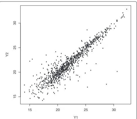
Figure 1 shows the log-scale scatter plot of the tech-nically duplicated samples under the same biological

15 20 25 30 15 20 25 30 Y1 Y2

Figure 1Scatter plot of duplicate samples.File: Scatter.pdf -Scatter plot of duplicate samples after log2 transformation from mass spectrometry proteomics data.

condition from a MS experiment. The variability differs according to the intensity levels in the plot, so that the naive outlier detection method, ignoring the heterogene-ity of variabilheterogene-ity, may often miss true outliers at high levels and select false outliers at low levels. If a number of technical replicates for each peptide under the same biological condition can be obtained in MS experiments, the examination of outliers can be conducted for each peptide. However, a small number of replicates is usually conducted for MS experiments due to the high cost of experiments and the limited supply of biological samples. Cho et al. [4] proposed a more elaborate approach for detecting outliers with low false positive and negative rates in MS data to solve the problem when the number of technical replicates is two. The algorithm was devel-oped by utilizing quantile regression for duplicate MS experiments. The R package (called OutlierD) that was also developed can only be used for duplicate experi-ments. Therefore, we here propose a new outlier detec-tion algorithm formultiplehigh-throughput experiments, particularly those with few, but more than two replicates.

Classical Approaches

Suppose that there arenreplicated samples andppeptides in MS data. Then letxijbe theith replicated sample from experiments under the same biological or experimental condition, wherei=1,. . .,nandj=1,. . .,p. For conve-nience, letyij=log2(xij). Typically,nis small andpis very large in high-throughput data,i.e.,p>>n. In addition, let y(1)j ≤y(2)j ≤ · · · ≤y(n)jbe ordered samples for peptide j, wherey(1)j = min1≤i≤nyijandy(n)j =max1≤i≤nyij, the smallest and the largest observations, respectively.

Outliers are often detected by the classical approaches such as Dixon’s Range Test and Grubbs test. Dixon’s Range Test, also known as Dixon’s Q-test [3], utilizes order statistics as follows.

Qj= (

y(2)j−y(1)j)

(y(n)j−y(1)j) or

(y(n)j−y(n−1)j)

(y(n)j−y(1)j) . (1) The denominator is the difference between the largest and smallest observations and the numerator is the difference between the smallest two values or the largest two values. If the test statistic Qj is smaller than the critical value given by Rorabacher [5], peptidejis flagged as an outlier. If n=2, the statistic is always 1; thus, this test is applicable forn≥3.

Grubbs’ test [2,6] also utilizes order statistics and its test statistic is defined as follows.

Tnj= (y(n)j− ¯y·j) sj

and T1j= (¯

y·j−y(1)j)

sj

, (2)

wherey¯·jis the sample mean andsjthe standard deviation for peptidej. The denominator is the standard deviation and the numerator is the difference between the small-est (or largsmall-est) value and the sample mean. If Tnj orT1j is smaller than the critical value, peptidejis flagged as an outlier. Ifn=2, the statistic is always 1/√2; thus, this test is also applicable forn≥3.

Proposed Methods

In duplicated experiments (n = 2), two observed values, x1jandx2jfor eachj, should be theoretically identical, but are not identical in practice due to their variability. Even though they are not identical, they should not differ sub-stantially. The tolerance of the difference between the two observed values from the same condition is not constant because their variability is heterogeneous. The variability of high-throughput data depends on intensity levels.

Cho et al. [4] proposed the construction of lower and upper fences using quantile regression in an MA plot with M and A values in vertical and horizontal axes, respectively, whereMjis the difference between replicated samples forjandAjis the average,i.e.,Mj = y1j−y2j = log₂(x1j/x2j) andAj = (y1j+y2j)/2 = (1/2)log2(x1jx2j) to detect the outliers accounting for the heterogeneity of variability.

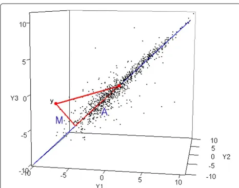
Figure 2Outlier detection using projection quantile regression. File: MA.pdf - Outlier detection using projection quantile regression for mass spectrometry data. The dotted lines representQ3(A)and the solid lines represent upper fences classifying outliers and non-outliers.

component (PC) becomes the center of each intensity level,i.e., a new axis for intensity levels. The experiments are replicated under the same biological and technical condition; hence, most variation can be explained by the first PC. It implies that it is enough to use the first PC practically. An outlier will have a large distance from its projection. Following the notations for applying quantile regression, we can define the distance of peptidejto the projection asMj and the length of the projection on the new axis as Aj. Then the first and third quantiles can be obtained by applying quantile regression on an MA plot withM and A in the vertical and horizontal axes, repectively; hence, the upper and lower fences can be constructed to classify the outliers.

Describing this projection approach in more detail, we first subtract the sample mean of each sample from each observation to shift the sample mean to the origin because the PC go through the sample means. The first PC vector vcan be found on the new sample space fromy∗₁,. . .,y∗_n and the projection of each peptide on the vectorvcan be obtained. Then, we can calculate the length of the projec-tion,|y∗_jv|/√vv, and the length of the difference between a vector of peptidejand the projection,|yj∗−(y_j∗v/vv)v|.

The length of the projection is multiplied by the sign of y∗_jv to distinguish the positive and negative directions. The signed length of the project and the length of the dif-ference are defined asAjandMjof peptidej, respectively. Outlying peptides will have unduly largeMvalues. Judg-ing whether it is undue or not depends onAjbecause the variability ofMvalues is heterogeneous. Like OutlierD, we obtain first and third quantiles,Q1andQ3,

depend-ing on intensity levels, and then construct the upper and

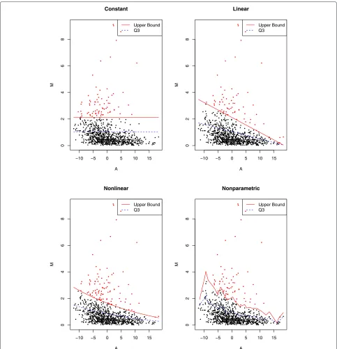
lower fences to classify outliers from normal observations. Quantile regression [7] is utilized on an MA plot to obtain the first and third quantile estimates,Q1(A) andQ3(A),

respectively, depending on the intensity levels A. The q-quantile linear quantile regression with {(Aj,Mj),j = 1,. . .,p}is used to find the parameters minimizing

{j:Mj≥g(Aj;θ0,θ1)}

q|Mj−g(Aj;θ0,θ1)| +

{j:Mj<g(Aj;θ0,θ1)}

(1−q)|Mj−g(Aj;θ0,θ1)| (3)

where 0 < q < 1, and g(Aj;θ0,θ1) = θ0 + θ1Aj.

Using Equation (3), the 0.25 and 0.75 quantile estimates, Q1(A) andQ3(A), are calculated depending on the

lev-elsA. Then, the lower and upper fences are constructed: Q1(A)−kIQR(A)andQ3(A)+kIQR(A), whereIQR(A)=

Q3(A)−Q1(A)andkis a tuning parameter. We setkto

1.5 as the default value in our algorithm and software pro-gram because the value is practically often used. A largerk value selects fewer peptides, while a smallerkselects more outliers. The value can be adjusted empirically according to the magnitude of the variation of the data.

We can obtain more flexible quantile estimates by non-linearandnonparametricquantile regression approaches [8]. For nonlinear quantile regression, the asymptotic function [9] can be employed:

g(Aj;θ1,θ2,θ3)=θ1{1−exp[−exp(θ2)×(Aj−θ3)]},

where θ1 is the asymptote, θ2 is the log rate, and θ3 is

the value of A at which the response becomes zero. In addition, Self-starting, Frank, Asymptotic with Offset and Copula functions can be employed. For nonparametric quantile regression, we utilize smoothing spline with the total variation regularization for univariate data to our algorithm [10]. A smoothing parameter plays a role in adjusting the degree of smoothness. We set it to 1 as the default, but it can be changed by users. The algorithm using projection can be summarized as follows.

Proposed Algorithm

1. Shift the sample means(y¯1,. . .,y¯n)to the origin (0,. . ., 0),i.e.,y∗_ij=yij− ¯yi.

2. Find the first PC vectorvusing PCA on the space of y∗₁,. . .,y∗n.

3. Obtain the projection of a vectory∗_j =(y₁∗_j,. . .,y∗_nj) of each peptidej onv, wherej=1,. . .,p.

4. Compute the signed length of the projection Aj=sign(y∗jv)|y∗jv|/

√

−10 −5 0 5 10 15

02468

Constant

A

M

Upper Bound Q3

−10 −5 0 5 10 15

02468

Linear

A

M

Upper Bound Q3

−10 −5 0 5 10 15

02468

Nonlinear

A

M

Upper Bound Q3

−10 −5 0 5 10 15

02468

Nonparametric

A

M

Upper Bound Q3

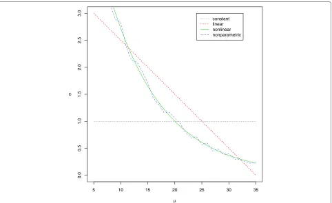
Figure 3Relationship between mean and variance for simulated data.File: Var.pdf - Constant, linear, nonlinear, and nonparametric relationship betweenμandσto generate the simulated data.

projectionMj= |y∗j −(yj∗v/vv)v|, where

j=1, 2,. . .,p.

5. Obtain the first and third quantile valuesQ1(A)and

Q3(A), on an MA plot using a quantile regression

approach. Then calculateIQR(A)=Q3(A)−Q1(A).

6. Construct the lower and upper fences,

LB(A)=Q1(A)-kIQR(A)andUB(A)=Q3(A)+

kIQR(A), wherek is a tuning parameter.

7. Declare peptidej as an outlier if it is located above the upper fence or under the lower fence.

Table 1 Sensitivities, specificities, and accuracies of the quantile and projection quantile methods for the simulated data from duplicated experiments

Simulated Under

n Method Constant Linear Nonlinear Nonparametric

Quantile

Constant (85.0, 99.5, 98.8) (84.7, 93.1, 92.6) (94.3, 87.6, 87.9) (94.3, 87.7, 88.0)

Linear (85.0, 99.5, 98.8) (83.7, 99.3, 98.5) (87.7, 94.7, 94.4) (87.3, 94.7, 94.3)

Nonlinear (85.0, 99.5, 98.8) (83.3, 99.3, 98.5) (87.7, 94.8, 94.5) (86.9, 94.9, 94.5)

Nonparametric (79.0, 99.2, 98.2) (81.6, 99.1, 98.2) (84.8, 99.0, 98.3) (84.8, 99.0, 98.3)

2 Projection Quantile

Constant (88.9, 99.1, 98.6) (69.7, 97.0, 95.7) (78.6, 94.1, 93.4) (78.8, 94.1, 93.3)

Linear (88.8, 99.1, 98.5) (86.5, 98.9, 98.3) (88.5, 96.1, 95.7) (88.2, 96.1, 95.7)

Nonlinear (88.8, 99.1, 98.5) (86.5, 98.9, 98.3) (88.3, 98.0, 97.6) (87.9, 98.0, 97.4)

Nonparametric (83.2, 98.7, 97.9) (84.4, 98.7, 98.0) (86.6, 98.6, 98.0) (86.0, 98.5, 97.9)

Results and discussion

We conducted a simulation study to investigate the performance of the proposed approaches. We also applied it to real-life data with three replicates of liquid chro-matography/tandem MS (LC-MS/MS) experiments.

Simulated data

Suppose that there are replicated samples with p =

1000 peptides. We considered two or more replicates,i.e., n ≥ 2. Assimilating reality, we first drew the meansμ_j from U(5, 35) and computed the variances σ_j2 with the

5 10 15 20 25 30 35

0.0

0.5

1.0

1

.5

2.0

2

.5

3.0

μ

σ

constant linear nonlinear nonparametric

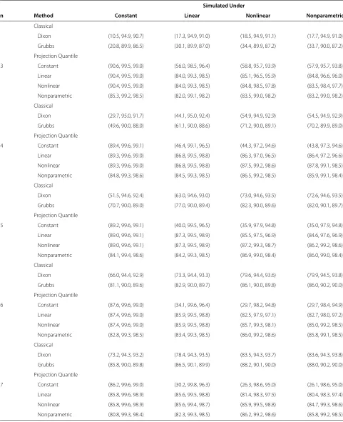
Table 2 Sensitivities, specificities, and accuracies of the classical and projection quantile methods for the simulated data from multiple experiments

Simulated Under

n Method Constant Linear Nonlinear Nonparametric

Classical

Dixon (10.5, 94.9, 90.7) (17.3, 94.9, 91.0) (18.5, 94.9, 91.1) (17.7, 94.9, 91.0)

Grubbs (20.8, 89.9, 86.5) (30.1, 89.9, 87.0) (34.4, 89.9, 87.2) (33.7, 90.0, 87.2)

Projection Quantile

3 Constant (90.6, 99.5, 99.0) (56.0, 98.5, 96.4) (58.8, 95.7, 93.9) (57.9, 95.7, 93.8)

Linear (90.4, 99.5, 99.0) (84.0, 99.3, 98.5) (85.1, 96.5, 95.9) (84.8, 96.6, 96.0)

Nonlinear (90.4, 99.5, 99.0) (84.0, 99.3, 98.5) (84.8, 98.5, 97.8) (83.5, 98.4, 97.7)

Nonparametric (85.3, 99.2, 98.5) (82.0, 99.1, 98.2) (83.5, 99.0, 98.2) (83.2, 99.0, 98.2)

Classical

Dixon (29.7, 95.0, 91.7) (44.1, 95.0, 92.4) (54.9, 94.9, 92.9) (54.5, 94.9, 92.9)

Grubbs (49.6, 90.0, 88.0) (61.1, 90.0, 88.6) (71.2, 90.0, 89.1) (70.2, 89.9, 89.0)

Projection Quantile

4 Constant (89.4, 99.6, 99.1) (46.4, 99.1, 96.5) (44.3, 97.2, 94.6) (43.8, 97.3, 94.6)

Linear (89.3, 99.6, 99.0) (86.8, 99.5, 98.8) (86.3, 97.0, 96.5) (86.4, 97.2, 96.6)

Nonlinear (89.3, 99.6, 99.0) (86.8, 99.5, 98.8) (87.5, 99.2, 98.6) (87.8, 99.1, 98.5)

Nonparametric (84.8, 99.3, 98.6) (84.5, 99.3, 98.5) (86.5, 99.2, 98.5) (85.9, 99.1, 98.4)

Classical

Dixon (51.5, 94.6, 92.4) (63.0, 94.6, 93.0) (73.0, 94.6, 93.5) (72.6, 94.6, 93.5)

Grubbs (70.7, 90.0, 89.0) (77.0, 90.0, 89.4) (82.3, 90.0, 89.6) (82.0, 90.1, 89.7)

Projection Quantile

5 Constant (89.2, 99.6, 99.1) (40.0, 99.5, 96.5) (35.9, 97.9, 94.8) (35.0, 97.9, 94.8)

Linear (89.0, 99.6, 99.1) (87.3, 99.5, 98.9) (85.5, 97.5, 96.9) (84.6, 97.6, 96.9)

Nonlinear (89.0, 99.6, 99.1) (87.3, 99.5, 98.9) (87.2, 99.3, 98.7) (86.2, 99.2, 98.6)

Nonparametric (84.1, 99.4, 98.6) (84.2, 99.3, 98.5) (86.9, 99.0, 98.4) (86.0, 99.0, 98.4)

Classical

Dixon (66.0, 94.4, 92.9) (73.3, 94.4, 93.3) (79.6, 94.4, 93.6) (79.9, 94.5, 93.8)

Grubbs (81.1, 90.0, 89.6) (82.9, 90.0, 89.7) (86.1, 90.0, 89.8) (86.0, 90.2, 90.0)

Projection Quantile

6 Constant (87.6, 99.6, 99.0) (34.1, 99.6, 96.4) (29.7, 98.2, 94.8) (29.7, 98.4, 94.9)

Linear (87.4, 99.6, 99.0) (85.9, 99.5, 98.8) (82.5, 97.9, 97.1) (82.7, 98.0, 97.2)

Nonlinear (87.4, 99.6, 99.0) (85.9, 99.5, 98.8) (85.7, 99.3, 98.1) (85.0, 99.2, 98.5)

Nonparametric (82.8, 99.3, 98.5) (83.4, 99.3, 98.5) (86.0, 99.2, 98.6) (85.8, 99.1, 98.5)

Classical

Dixon (73.2, 94.3, 93.2) (78.4, 94.3, 93.5) (83.5, 94.3, 93.7) (83.6, 94.3, 93.8)

Grubbs (85.8, 90.0, 89.8) (86.5, 90.1, 89.9) (88.2, 90.1, 90.0) (88.0, 90.2, 90.0)

Projection Quantile

7 Constant (86.2, 99.6, 99.0) (30.2, 99.8, 96.3) (26.3, 98.6, 95.0) (26.1, 98.6, 95.0)

Linear (85.8, 99.6, 98.9) (85.6, 99.5, 98.8) (81.4, 98.3, 97.5) (80.4, 98.3, 97.4)

Nonlinear (85.8, 99.6, 98.9) (85.6, 99.4, 98.7) (85.9, 99.5, 98.8) (84.7, 99.3, 98.6)

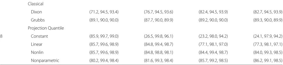
Table 2 Sensitivities, specificities, and accuracies of the classical and projection quantile methods for the simulated data

from multiple experiments(Continued)

Classical

Dixon (71.2, 94.5, 93.4) (76.7, 94.5, 93.6) (82.4, 94.5, 93.9) (82.7, 94.5, 93.9)

Grubbs (89.1, 90.0, 90.0) (87.7, 90.0, 89.9) (89.2, 90.0, 90.0) (89.3, 90.0, 89.9)

Projection Quantile

8 Constant (85.9, 99.7, 99.0) (26.5, 99.8, 96.1) (23.2, 98.0, 94.2) (24.1, 97.9, 94.2)

Linear (85.7, 99.6, 98.9) (84.8, 99.4, 98.7) (77.1, 98.1, 97.0) (77.3, 98.1, 97.1)

Nonlin (85.7, 99.6, 98.9) (84.8, 98.8, 98.1) (84.4, 99.4, 98.7) (84.0, 99.3, 98.5)

Nonparametric (80.2, 99.4, 98.4) (81.6, 99.3, 98.4) (85.7, 99.2, 98.5) (86.2, 99.1, 98.5)

following relationships between the meanμand variance σ2.

Constant: σ_j=1

Linear: σ_j= −(μ_j−5)/10+3 Nonlinear: σ_j=exp(2−μ_j/10)

Nonparametric: σ_j=exp(2−μ_j/10)+(2Bj−1)Zj

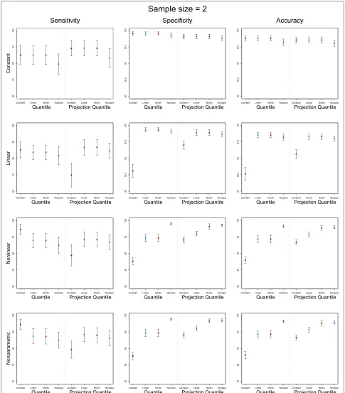
whereBj ∼ Bernoulli(1/2)andZj ∼ N(1/μj, 0.01). The relationships between the means and the variances are shown in Figure 3. For 950 non-outliers (j = 1,. . ., 950), we assumed thatYij ∼ N(μj,σj2) fori = 1,. . .,n. For 50 outliers (j = 951,. . ., 1000), we assumed thatYij ∼ N(μ_j,σ_j2)for one of the samples andYij ∼ N(μj,σj2)for the other samples, whereμj ∼ U(5, 35) andμj = μj+ (2Bj−1)U(1, 2)for constant variance andμj=μj+(2Bj− 1)(120/μj)U(1, 2) for other variances. Thus, an artificial data set for eachnwas generated with 950 non-outliers and 50 outliers. Then, the data were used to check the sen-sitivities (the probabilities of detecting outliers correctly), specificities (the probabilities of detecting non-outliers correctly), and accuracies (the probabilities of detecting outliers or non-outliers correctly) of the quantile and pro-jection quantile approaches for n = 2 and the Dixon test, Grubbs’s test, and projection quantile approaches for n=3,. . ., 8. Constant, linear, nonlinear, and nonparamet-ric quantile regressions were accounted for the quantile and projection quantile approaches. This procedure was repeated 1000 times independently.

Table 1 presents the sensitivities, specificities, and accu-racies of the quantile and projection quantile methods for the simulated data from duplicated experiments (n= 2) and Figure 4 shows their confidence intervals. The classical methods were not applied because they work only for n > 2. Under the constant variance, all the methods performed well. Under the linear, nonlinear, and nonparametric variances, the quantile and projection quantile methods with constant quantile regression per-formed worse than those with the other quantile regres-sion due to the heterogeneity of the variability, as shown in Cho et al. [4]. When comparing the quantile and

projection quantile methods, the latter sometimes had somewhat lower sensitivities than the former. However, the quantile and projection quantile methods are mostly comparable.

Table 2 presents the sensitivities, specificities, and accu-racies of the classical and projection quantile methods for the simulated data from three to eight experiments (3 ≤ n ≤ 8) and Additional File 1 shows their confi-dence intervals. The results are not shown for n ≥ 9. With multiple experiments, the projection quantile meth-ods with constant, linear, nonlinear, and nonparametric quantile regression performed like those with duplicated experiments. Whenn=3, the classical methods had very low sensitivities, resulting in the lower accuracies. With increasing n, the sensitivities of the classical methods increased. Whenn=7 or 8, Glubbs’ test was comparable to the projection quantile methods with linear, nonlinear, and nonparametric quantile regression. This implies that the classical methods require a sufficiently large number of replicates. In reality, experiments are often repeated three or more times; thus, the projection quantile method is practically very useful.

Real-life data

We here illustrate the projection quantile approach with real-life data obtained from three replicates of LC/MS/MS experiments with 922 peptides (n=3 andp=922). The details of the experiments can be found in Min et al. [11] and Cho et al. [4]. Here, the primary goal of the analysis is to detect outliers automatically in the pre-processing step prior to further analysis.

Figure 53-D Scatter plot of LC/MS data with three replicates.File: Scatter3d.png - Scatter plot of LC/MS data with three replicates; The straight line at the center is the first PC vector. C = Contant, L = Linear, NL = Nonlinear, NP = Nonparametric.

tended to select more peptides at low levels as outliers, whereas the others selected more peptides at the higher levels.

quantile regression is more appropriate than constant quantile regression.

Conclusion

We propose an approach for detecting outliers automat-ically in low replicated, high-throughput data generated from MS experiments. Because of the practical problems such as cost and time, LC/MS data is usually generated by repeating the experiment three or four times under the same technical or biological condition. Outliers can be investigated within each peptide when there are many replicates; however, within-peptide approaches such as Dixon and Grubbs’ tests are crude in the case of few repli-cates. A quantile regression approach on an MA plot was proposed in Cho et al. [4] when there are only two repli-cates. Thus, our proposed method can be used when there are two or somewhat more replicates.

The projection approach using various quantile regres-sions was examined for outlier detection. The projection approach with linear, nonlinear, or nonparametric quan-tile regression was more appropriate than the others in heterogeneous high-throughput data. The choice among linear, nonlinear, and nonparametric is dependent on the degree of heterogeneity of the data. In addition, our soft-ware program provides a number of options. A single method may not be the best in any situation. There-fore, the data can be applied empirically with various options. Moreover, experimental confirmation is needed after applying our automatic outlier detection. Never-theless, it is useful because manual examination of all observations is time-consuming without pre-screening.

Availability and Requirements

Project name:Outlier Detection for Mass Spectrometry Project homepage:http://statlab.korea.ac.kr/OutlierDM/ Operating system(s): Windows, Unix-like systems (Linux, Mac OS X)

Programming language:R (the version of R should be ¿= 2.14.0)

License:GNU GPL version 2 or later

Additional material

Additional file 1: Confidence intervals of the sensitivities,

specificities, and accuracies for multiple experiments.File: CI3.pdf

-Mean plus or minus one standard error of the sensitivities, specificities, and accuracies of the classical and projection quantile methods for the simulated data from multiple experiments (3≤n≤8).

Competing interests

The authors declare that they have no competing interests.

Author’s contributions

Cho designed and directed this research. Eo wrote and optimized the R code and maintained the software program. Cho and Eo wrote the manuscript. All authors contributed ideas, and read and approved the manuscript.

Acknowledgements

This research was supported by the Basic Science Research Program through the National Research Foundation of Korea (NRF) funded by the Ministry of Education, Science and Technology (2010-0007936).

Received: 6 January 2012 Accepted: 18 April 2012 Published: 15 May 2012

References

1. Barnett V, Lewis T:Outliers in Statistical Data. Hoboken, NJ, USA: Wiley Series in Probability & Statistics, John Wiley & Sons; 1984.

2. Grubbs FE:Sample criteria for testing outlying observations.The Annals of Mathematical Statistics1950,21:27–58.

3. Dixon WJ:Analysis of extreme values.The Annals of Mathematical Statistics1950,21:488–506.

4. Cho H, Kim YJ, Jung HJ, Lee SW, Lee JW:OutlierD: an R package for outlier detection using quantile regression on mass spectrometry

data.Bioinformatics2008,24(6):882–884.

5. Rorabacher DB:Statistical Treatment for Rejection of Deviant Values: Critical Values for Dixon’s Q parameter and Related Subrange Ratios

at the 95% Confidence Level.Anal Chem1991,63:139–146.

6. Grubbs FE:Procedures for Detecting Outlying Observations in

Samples.Technometrics1969,11:1–21.

7. Koenker R, Bassett G:Regression quantiles.Econometrics1978,46:33–50. 8. Koenker R:Quantile Regression. Cambridge, United Kingdom: Econometric

Society Monograph Series, Cambridge University Press; 2005. 9. R Development Core Team:R: A Language and Environment for Statistical

Computing. Vienna, Austria: R Foundation for Statistical Computing; 2011. [ISBN 3-900051-07-0]. [http://www.R-project.org/].

10. Koenker R, Ng P, Portnoy S:Quantile Smoothing Splines.Biometrika 1994,81:673–680.

11. Min HK, Hyung SW, Shin JW, Nam HS, Ahm SH, Jung HJ, Lee SW:

Ultrahigh-pressure dual online solid phase extraction/capillary reverse-phase liquid chromatography/tandem mass spectrometry (DO-SPE/cRPLC/MS/MS): A versatile separation platform for high-throughput and highly sensitive proteomic analyses.

Electrophoresis2007,28:1012–1021.

doi:10.1186/1756-0500-5-236

Cite this article as:Eoet al.:Outlier Detection using Projection Quantile

Regression for Mass Spectrometry Data with Low Replication.BMC Research

Notes20125:236.

Submit your next manuscript to BioMed Central and take full advantage of:

• Convenient online submission

• Thorough peer review

• No space constraints or color figure charges

• Immediate publication on acceptance

• Inclusion in PubMed, CAS, Scopus and Google Scholar

• Research which is freely available for redistribution