T E C H N I C A L N O T E
Open Access
MetabR: an R script for linear model analysis of
quantitative metabolomic data
Ben Ernest
1,2, Jessica R Gooding
3, Shawn R Campagna
3, Arnold M Saxton
1,2and Brynn H Voy
1,2*Abstract
Background:Metabolomics is an emerging high-throughput approach to systems biology, but data analysis tools are lacking compared to other systems level disciplines such as transcriptomics and proteomics. Metabolomic data analysis requires a normalization step to remove systematic effects of confounding variables on metabolite measurements. Current tools may not correctly normalize every metabolite when the relationships between each metabolite quantity and fixed-effect confounding variables are different, or for the effects of random-effect confounding variables. Linear mixed models, an established methodology in the microarray literature, offer a standardized and flexible approach for removing the effects of fixed- and random-effect confounding variables from metabolomic data.
Findings:Here we present a simple menu-driven program,“MetabR”, designed to aid researchers with no programming background in statistical analysis of metabolomic data. Written in the open-source statistical
programming language R, MetabR implements linear mixed models to normalize metabolomic data and analysis of variance (ANOVA) to test treatment differences. MetabR exports normalized data, checks statistical model
assumptions, identifies differentially abundant metabolites, and produces output files to help with data interpretation. Example data are provided to illustrate normalization for common confounding variables and to demonstrate the utility of the MetabR program.
Conclusions:We developed MetabR as a simple and user-friendly tool for implementing linear mixed model-based normalization and statistical analysis of targeted metabolomic data, which helps to fill a lack of available data analysis tools in this field. The program, user guide, example data, and any future news or updates related to the program may be found at http://metabr.r-forge.r-project.org/.
Keywords:R script, User-friendly, Linear mixed model, Statistics, Normalization, Mass spectrometry-based metabolomics
Findings
Background
Quantitative metabolomics is a high-throughput approach to systems biology in which many small molecules (metabolites) from a biological sample are simultaneously measured, commonly using nuclear magnetic resonance spectroscopy (NMR), gas chromatography—mass spec-trometry (GC-MS), or liquid chromatography—mass spec-trometry (LC-MS). While transcriptomics and proteomics
are established approaches for characterizing the effects of experimental conditions on metabolism, gene and protein expression changes merely indicate the potential for changes in metabolic endpoints. Metabolic changes are “real-world”endpoints, so metabolomics can connect these functional genomics platforms with actual physiology [1].
LC-MS metabolomic approaches fall into two catego-ries: those that attempt to measure every metabolite in the sample (untargeted approaches) and those that attempt to measure only a subset of the metabolites (targeted approaches) [2]. A key benefit of targeted ap-proaches is that the detected metabolites can also be rea-dily quantified. Like other approaches to systems biology that rely on the analysis of multiple samples to generate large datasets, two important issues hold true in targeted * Correspondence:[email protected]
1
Graduate School of Genome Science and Technology, University of Tennessee, Knoxville, TN 37996, USA
2
Department of Animal Science, University of Tennessee, Knoxville, TN 37996, USA
Full list of author information is available at the end of the article
metabolomics. First, experiments frequently are carried out in multiple “blocks”. For example, targeted LC-MS metabolomic platforms involve lengthy instrumental runs and may rely on multiple runs to enhance metabolite coverage [3,4], often necessitating multiple run days to analyze all samples. Each run day represents a different block, which introduces technical variability in metabolite detection signals from day-to-day variances in factors related to the instrument’s operation, such as injection volume and ionization efficiency. Second, sampling and measurement variables introduce technical variability in metabolite detection signals, including tissue mass (for multicellular organisms), cell number and size (for micro-organisms), sample matrix effects, and mass spectrometer variability (measured by the signal from an internal stan-dard present in the metabolite extraction solvent in our experiments). Clearly, the metabolite signal variability due to block and sampling/measurement variables needs to be distinguished from variability due to experimental treat-ment factors, which calls for a normalization step to re-move the effects of such confounding variables.
Conventional LC-MS metabolomic data normalization is carried out by expressing each metabolite signal rela-tive to values of sampling/measurement variables [3,4]. Statistical tests for mean differences between treatment groups are performed on normalized metabolite values, with metabolite means averaged across the levels of any block factors (i.e., run day).
There are limitations to this conventional normaliza-tion approach, however. First, often many metabolites are normalized to one internal standard (i.e., one for all positive ions and one for all negative ions). This would introduce additional bias if there were low or negative correlation between the internal standard signal and a metabolite signal (i.e., for metabolites with different che-mical properties from the internal standard), or if the internal standard signal differed significantly between treatment groups. Second, while ignoring block factors (i.e., comparing metabolite means averaged across sam-ples analyzed on different days) increases sample size, significant block effects on metabolite signals may widen confidence intervals, which may preclude identification of “significant” metabolites and conceal statistical out-liers. Block effects may dramatically bias the data, espe-cially if they are not balanced across treatment groups.
Currently available software packages provide power-ful tools for pre-processing (i.e., peak selection and in-tegration and retention time alignment), visualization (i.e., biochemical pathway mapping), and/or interpreta-tion of targeted and untargeted metabolomic data [5-10]. However, these packages have limitations because they ei-ther 1) do not provide normalization tools for removing confounding effects of experimental variables [7-9]; 2) use the conventional normalization approach [6]; or 3) require
the researcher to manually determine a normalization fac-tor for each experimental sample [5].
A flexible and standardized normalization approach that improves on current limitations would improve metabolo-mic analyses. An efficient and intuitive approach to con-trol for confounding variables is to estimate their effects on metabolite signals using linear models. Rather than as-suming similar relationships between each metabolite sig-nal and confounding variables, a linear model fit for each metabolite can be used to estimate and partition the effects of each experimental variable, including treatment factor, on each metabolite signal. Further, experimental variables can be modeled as having either a fixed or random effect on metabolite signals, with important im-plications. Fixed-effect variables are assumed to have a constant effect on metabolite signals, influence metabolite signals in an anticipated direction, and have a similar in-fluence in replicate experiments. Common fixed-effect variables are number of cells, tissue mass, and ionization efficiency. By comparison, the effects of random-effect variables cannot be anticipated a priori, and they create variation, but overall do not influence metabolite signals. Typical examples are specimen gender, species or line, ex-periment day, instrument, and technician [11], although some of these could be treated as hypothesis-driven ex-perimental factors in some experiments.
Mixed models can be used to estimate the effects of fixed- and random-effect variables on a response variable [11] and are an established approach for normalizing mi-croarray data [12-21]. For two primary reasons, however, currently available microarray data normalization tools are not suitable for metabolomic data. First, microarray normalization tools adjust data for systematic effects spe-cific to microarray technology, such as “dye bias” of dif-ferent fluors, spatial position effects on the microarray chip, background signals, and biases due to probe binding strengths [22]. Second, microarray normalization tools are often platform specific, designed to carry out pre-proces-sing and quality control only for Illumina BeadArray or for Affymetrix GeneChip platforms, for example [23].
Methods
Implementation of MetabR
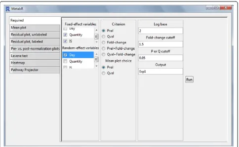
A graphical user interface (GUI)-based program, MetabR (Additional file 1), was written in the R open-source lan-guage (version 2.15). A screenshot of the GUI is shown in Figure 1. The GUI was built using the “gWidgets” package [24]. As described in the user guide (Additional file 2), the GUI is used to select which variables to define in a normalization model as fixed- and random-effect variables and to tailor statistical analysis to the resear-cher’s needs. As a threshold to screen for metabolites that differ significantly in abundance between treatment groups, the researcher may choose p-value, q-value, mean fold-change, or a combination of p-value or q-value and mean fold-change, as well as the specific values of these thresholds.
In this program, either a fixed linear model (function “lm”in the“stats”package) or a linear mixed model (func-tion“lmer”in the“lme4”package) [25] is constructed that includes the normalization variables selected by the user, and one Group treatment factor, for example
Metabolite ¼ μ þ Group þ β∗Quantity þ βIS
þ Day þ e; whereμ= group mean,
Group = treatment factor,
Quantity = a measured, continuous value of the amount of tissue used to produce each sample,
IS = a measured, continuous value of the detection sig-nal from an intersig-nal standard present in the metabolite extraction solvent,
Day = a normalization factor accounting for the effects of different run days on metabolite signals,
and e = residual error.
The residuals and treatment group means from the fit-ted model are added together to yield normalized data, which adjusts for effects of sample quantity, ionization efficiency, and run day, as appropriate for the experi-mental design of the study.
[image:3.595.57.541.416.714.2]To check normality and equal variance assumptions made by linear models, R functions “shapiro.test” in the “stats” package (“stats”and any other packages not refer-enced are part of R [26]) and“levene.test”in the“lawstat” package [27] are used, respectively. In addition, resi-dual error plots are produced, and normalized data are exported for possible secondary use by the researcher. Tukey’s Honest Significant Difference (HSD; function “TukeyHSD” in the“stats” package) method is used to test for treatment group mean differences in the nor-malized data based on the Studentized range statistic. Q-values [28] are calculated from the list of Tukey HSD
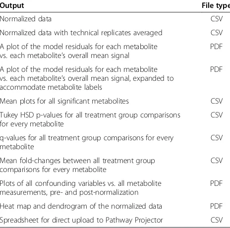
p-values for each treatment group comparison using the “qvalue” function in the “qvalue” package [28]. If any treatment group mean is significantly different from any other, a group mean plot with confidence intervals is constructed for the metabolite. Differences among treat-ment group means are represented by letter groupings generated by code adapted from a SAS macro [29], with means that share any letter being statistically equal. Fur-ther, statistical results from“significant” metabolites are exported into a spreadsheet that can be directly uploaded to Pathway Projector [9], which uses the information to map the metabolites, colored dots representing the di-rection and size of mean fold-changes, and either p- or q-values, to biochemical pathways. The program generates a series of files listed in Table 1 and described in the user guide (Additional file 2).
Experimental data collection
Two experimental datasets were generated in our lab to illustrate the utility of MetabR. In both experiments, adi-pose tissue samples were flash frozen in liquid nitrogen and powdered with a mortar and pestle before meta-bolite extraction, which followed a previously described procedure [30]. The extracted metabolomes were then analyzed by liquid chromatography—tandem mass spec-trometry (LC-MS/MS) via a slightly modified version of the methods of Rabinowitz and co-workers [30-32] that scans for approximately 350 total metabolites in positive and negative ionization modes. The Quan Browser func-tion in the Xcalibur software package (Thermo Scientific, Waltham, MA) was used to assess the presence of each metabolite based on standard detection parameters, such
as retention time, signal-to-noise ratio, and peak shape. Signal intensity in ion counts was then determined using Xcalibur to manually integrate each peak, and these data were exported into a Microsoft Excel spreadsheet for stat-istical analysis.
The first experiment was designed to examine the effects of dietary restriction and insulin immunoneutrali-zation on adipose tissue metabolism in chickens. A total of 127 metabolites were detected in abdominal adipose tissue from 16- or 17-day-old male broiler chicks that were fedad libitum(“Control”), fasted for 5 hours (“Fast”), or immunoneutralized against the effects of endogenous insulin (“InsNeut”), as we previously described [33,34]. This study included two factors, Treatment and Day (day 1, day 2, or day 3). Fourteen metabolite measurements from this experiment are provided in Additional files 3 (“Chicken example data 1”) and 4 (“Chicken example data 2”), corresponding to metabolites detected in positive and negative ionization modes, respectively.
The second experiment was designed to examine the effects of Bisphenol A (BPA) on adipose tissue metabo-lism in mice. A total of 93 metabolites were detected in abdominal adipose tissue from 32 16-week-old inbred male mice which, from weaning, were fed ad libitum
and given drinking water spiked with 0, 0.05, 0.5, or 5μM BPA. Sixteen mice from each of the inbred strains C57BL/6J and DBA/2J were used in this study. A few missing values arose when a metabolite was not detected in a subset of the samples. Using a zero value for these measurements would bias the results, so they were set to missing (“NA”) which excludes that measurement from analysis. This study included three factors, Treat-ment, Strain (C57BL/6J or DBA/2J), and Day (day 1, day 2, day 3, or day 4). Twelve metabolite measurements from this experiment are provided in Additional files 5 (“Mouse example data 1”) and 6 (“Mouse example data 2”), corresponding to metabolites detected in positive and negative ionization modes, respectively.
Modeling confounding variables as fixed- vs. random-effect In our chicken example, Group, Quantity, and IS were modeled as fixed-effect variables, while Day was mo-deled as a random-effect variable. To illustrate the dif-ference, if Day is defined as a fixed-effect variable, the estimated treatment group mean includes the average Day effects, and the variance and corresponding confi-dence intervals are based only on residual error and sample size. Inferences about treatment effects refer only to the days used in the experiment. If Day is defined as a random-effect variable, the estimated mean no longer includes Day. Instead, the Day effect becomes a source of random variation that is added to the variance of the estimated mean. The variance and confidence intervals are larger than those when Day is treated as a
fixed-Table 1 Output files produced by the MetabR program
Output File type
Normalized data CSV
Normalized data with technical replicates averaged CSV A plot of the model residuals for each metabolite
vs. each metabolite’s overall mean signal
A plot of the model residuals for each metabolite vs. each metabolite’s overall mean signal, expanded to accommodate metabolite labels
Mean plots for all significant metabolites CSV
Tukey HSD p-values for all treatment group comparisons for every metabolite
CSV
q-values for all treatment group comparisons for every metabolite
CSV
Mean fold-changes between all treatment group comparisons for every metabolite
CSV
Plots of all confounding variables vs. all metabolite measurements, pre- and post-normalization
effect variable, but experimental results can now be cor-rectly extrapolated to all possible days [11].
Results
Chicken experimental results
For the chicken data, Quantity (tissue mass) and IS (in-ternal standard measurement, Tris in positive ionization mode and Benzoic Acid in negative ionization mode)
were selected as fixed-effect regression variables, and Day (run day) as a random-effect factor.
[image:5.595.59.538.102.337.2]Summary information printed in the R console (not shown) includes 1) results from the Shapiro-Wilk test of normality; 2) results from Levene’s test of equality of variance; 3) pairwise mean fold-changes between all treatment groups for significant metabolites (also expor-ted into a spreadsheet; see Table 2 for the data); and 4)
Table 2 Chicken experiment fold-changes
Treatment comparison
Fast-control InsNeut-control InsNeut-fast Metabolite Fold-change P-value Fold-change P-value Fold-change P-value
ATP 1.273 0.384 1.059 0.932 0.832 0.588
Citraconate 0.969 0.694 0.982 0.915 1.014 0.907
Citrate 1.251 0.047 1.054 0.720 0.842 0.196
Dihexose 0.082 <0.001 0.590 0.928 7.217 0.001
Inosine 0.736 0.328 0.910 0.580 1.236 0.890
Lactate 0.873 0.137 0.991 0.974 1.135 0.198
Pyruvate 1.100 0.353 1.065 0.640 0.969 0.870
2-Oxoglutarate 0.929 0.754 1.511 0.001 1.627 <0.001
1-Methyladenosine 0.934 0.878 0.923 0.865 0.989 1.000
Glutamine 0.676 0.026 2.512 <0.001 3.715 <0.001
Guanosine 0.762 0.215 0.833 0.257 1.094 0.993
O-Acetyl-L-serine 0.614 0.337 2.276 0.085 3.707 0.004
Glucosamine 1.014 0.959 2.073 <0.001 2.044 <0.001
Thiamine 0.486 0.059 0.781 0.860 1.607 0.156
Mean fold-changes among the three treatment groups for the chicken example data (14 metabolites across positive and negative ionization modes), and associated Tukey HSD p-values for mean differences (bold values are p < 0.05).
[image:5.595.57.540.483.714.2]pairwise Tukey HSD p-values or q-values between all treatment groups for significant metabolites (also expor-ted into a spreadsheet; see Table 2 for the data). This printout showed that Shapiro-Wilk p-values for all meta-bolites were greater than 0.05, indicating no violation of the assumption of normality. Levene’s test p-values for Citraconate and Inosine were less than 0.05, indicating a possible violation of the linear model assumption of equality of variance. By using the diagnostic results from Shapiro-Wilk and Levene’s tests, researchers can identify when data are unacceptable for use with the linear
model approach. Ion counts are sometimes modeled as Poisson distributed, so if normality concerns are still an issue after opting for a log transformation, the re-searcher may wish to pursue an alternative statistical approach.
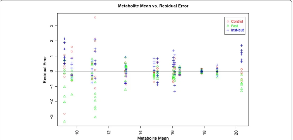
[image:6.595.57.291.88.296.2]Figure 2 contains the plot of residual error for each metabolite after data transformation and normalization in relation to the overall mean abundance for each me-tabolite across all samples (we used log base 2 transfor-mation). This plot can be used to determine whether data transformation and normalization corrected for the typical relationship of increasing variance with increa-sing mean. In this example, variance is visually relatively consistent across groups, and somewhat greater for low-abundance metabolites.
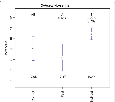
Figure 3 illustrates an example of the mean plots and 95% confidence interval bars created for metabolites with a statistically significant effect of treatment. O -Acetyl-L-serine levels were significantly lower in Fast samples compared to InsNeut. Mean separation letters indicate that Fast and InsNeut groups differed signifi-cantly from each other (p < 0.05 threshold chosen), but neither differed from Control. Fold-changes between treatment group means (not log transformed) are dis-played below the letters. Fold-changes in the nth row correspond to comparisons with the group in the nth column, (i.e., the mean ofO-Acetyl-L-serine was 3.707-fold higher in InsNeut compared to Fast).
Figure 4 shows a box-and-whisker plot of Citrate vs. run day, an ANOVA confounding variable, before and after data normalization with MetabR. Figure 5 shows a scatter plot of Pyruvate vs. Quantity, a regression con-founding variable, before and after data normalization with MetabR. These plots are produced automatically by MetabR for all metabolites and all confounding variables
[image:6.595.61.539.520.696.2]Figure 3Group mean plots forO-Acetyl-L-serine in the chicken experiment.Legend - Treatment group metabolite means, 95% confidence intervals, mean fold-changes, and significant difference letters are combined to summarize results for each significant metabolite.
Figure 5Pre- and post-normalization plots: metabolite vs. tissue quantity.Legend - Normalization removed the correlation between the quantity of tissue analyzed and the Pyruvate detection signal in the chicken experiment.
O−Acetyl−L−serine
Thiamine
ATP
Dihexose Glutamine
Citraconate
Lactate
1−Methyladenosine
Citrate
2−Oxoglutarate
Guanosine
Glucosamine
Inosine
Pyruvate
Fast_Chicken8 Fast_Chicken13 Control_Chicken6 Control_Chicken5 Control_Chicken2 Fast_Chicken11 Fast_Chicken9 Fast_Chicken10 Fast_Chicken14 Fast_Chicken12 InsNeut_Chicken18 InsNeut_Chicken17 InsNeut_Chicken15 InsNeut_Chicken21 InsNeut_Chicken19 Control_Chicken3 InsNeut_Chicken20 InsNeut_Chicken16 Control_Chicken1 Control_Chicken4 Control_Chicken7
−3 −1 1 2 3
Column Z−Score
Color Key
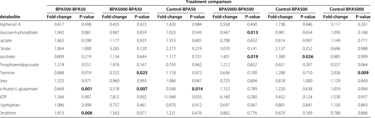
[image:7.595.60.537.291.666.2]Table 3 Mouse experiment fold-changes
Treatment comparison
BPA500-BPA50 BPA5000-BPA50 Control-BPA50 BPA5000-BPA500 Control-BPA500 Control-BPA5000
Metabolite Fold-change P-value Fold-change P-value Fold-change P-value Fold-change P-value Fold-change P-value Fold-change P-value
Bisphenol A 0.817 0.998 0.455 0.423 1.420 0.984 0.558 0.490 1.738 0.946 3.117 0.261
Glucose-6-phosphate 1.042 0.081 0.987 0.859 1.023 0.545 0.947 0.013 0.981 0.654 1.036 0.168
Lactate 1.663 0.298 1.177 0.923 1.353 0.401 0.708 0.652 0.814 0.997 1.149 0.771
Citrate 1.064 1.000 3.265 0.120 2.273 0.219 3.070 0.141 2.137 0.252 0.696 0.988
Isocitrate 0.809 0.219 1.134 0.644 1.117 0.731 1.401 0.019 1.380 0.026 0.985 0.999
Phosphoenolpyruvate 1.218 0.551 1.476 0.167 0.793 0.962 1.212 0.852 0.651 0.287 0.537 0.064
Thymine 0.868 0.919 0.552 0.025 1.118 0.972 0.636 0.100 1.288 0.710 2.026 0.009
Urea 1.325 0.971 0.960 0.993 1.084 0.947 0.725 0.894 0.818 1.000 1.129 0.849
N-Acetyl-L-glutamate 0.449 0.001 0.518 0.007 0.548 0.014 1.152 0.789 1.220 0.638 1.059 0.994
ADP 1.264 0.907 7.812 0.092 11.948 0.035 6.180 0.280 9.452 0.124 1.530 0.957
Tryptophan 1.086 0.998 0.757 0.461 0.870 0.912 0.697 0.367 0.801 0.841 1.150 0.843
Ornithine 1.813 0.008 1.563 0.071 1.231 0.476 0.862 0.776 0.679 0.189 0.788 0.686
Mean fold-changes among the four treatment groups for the mouse example data (12 metabolites across positive and negative ionization modes), and associated Tukey HSD p-values for mean differences (bold values are p < 0.05).
Research
Notes
2012,
5
:596
Page
8
o
f
1
0
ntral.com/1
included in the input data, and they give visual verifica-tion that the effects of confounding variables on metabo-lite measurements were removed by normalization using the linear model approach.
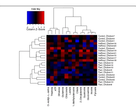
Figure 6 shows a heat map and dendrogram of the normalized data, produced automatically by MetabR via the“heatmap.2”function from the“gplots”package [35]. A heat map is useful for visualizing overall differences in metabolic signatures, and the dendrogram gives visual evidence of whether the experimental conditions signi-ficantly influenced metabolic signatures. Each metabolite plotted is mean-centered, helping to call attention to metabolites differing in abundance among samples. The chickens appear to cluster non-randomly based on their overall metabolic signatures (Figure 6). InsNeut chickens cluster in the upper half of the dendrogram, completely separate from Fast chickens, suggesting that these two treatment groups have distinct metabolic signatures, while the metabolic signature of the Control chickens appears less distinct.
Table 2 contains all between-group mean fold-changes for the metabolites, with differences tested by Tukey’s HSD at the 5% significance level. We produced this table by combining the mean fold-changes and p-values exported automatically by MetabR. As shown, the ex-periment had sufficient power to detect a fold-change as low as 1.25 for Citrate between Fast and Control groups. In general, the differences between the Control and InsNeut groups were smaller than other treatment group comparisons. The program exports q-values automa-tically, and the researcher may select p-value, q-value, mean fold-change, or a combination of either p-value or q-value and mean fold-change as a significance thres-hold. As technological improvements continue to allow more metabolites to be detected, the chance of false dis-coveries will increase, making false discovery corrections (q-value) increasingly necessary.
Mouse experimental results
MetabR was run on the mouse example data in Additional files 5 and 6, selecting the same parameters as the chicken experiment, except that “Strain” (C57BL/6J or DBA/2J) was additionally selected as a random-effect variable in order to remove the effects of different mouse strains on metabolite measurements. Two metabolites had Shapiro-Wilk p-values less than 0.05 and W statistics less than 0.90, indicating possible violations of normality. No meta-bolites were identified as having unequal variance among treatment groups. The residual plot (not shown) also showed no evidence of unequal variance, and it was vis-ually apparent that variance was equal across all measure-ment levels, and thus the log base 2 transformation chosen for the analysis was effective. Fold-change results are given in Table 3.
Conclusions
The open-source statistical computing software R [26] provides a convenient environment for statistical analysis of metabolomic and other -omic data. We developed a user-friendly R program that normalizes metabolomic data using linear mixed-effect modeling (with regression and ANOVA terms), statistically compares treatments, and exports results files to aid data interpretation, filling an important lack in statistical analysis tools available to the metabolomics community. The MetabR program file, example data, and user guide are available as an R-Forge project at http://metabr.r-forge.r-project.org/. This web-site will also contain future news or updates related to MetabR, including availability through the Comprehen-sive R Archive Network (CRAN) or Bioconductor.
Availability and requirements Project name:MetabR
Project home page:http://metabr.r-forge.r-project.org/
Operating system(s):Windows, Mac, Linux, any system that runs R
Programming language:R
Other requirements:Required R packages are installed automatically. The program was written and tested using R version 2.15 for Windows.
License:GNU General Public License (GPL)
Any restrictions to use by non-academics:No restrictions
Availability of supporting data
The datasets supporting the results of this article are included within the article (and its additional files).
Additional files
Additional file 1:MetabR.MetabR program file.
Additional file 2:User Guide.MetabR user guide.
Additional file 3:Chicken_pos.Chicken example data 1 from positive ionization mode.
Additional file 4:Chicken_neg.Chicken example data 2 from negative ionization mode.
Additional file 5:Mouse_pos.Mouse example data 1 from positive ionization mode.
Additional file 6:Mouse_neg.Mouse example data 2 from negative ionization mode.
Abbreviations
ANOVA: Analysis of variance; BPA: Bisphenol A; CSV: Comma-separated values; GUI: Graphical user interface; HSD: Honest Significant Difference; IS: Internal standard; LC-MS: liquid chromatography—mass spectrometry; LC-MS/MS: Liquid chromatography—tandem mass spectrometry.
Competing interests
Authors’contributions
BE wrote the program. BE, SRC, BHV, and JRG collaborated to outline the issues in data analysis and process all biological data. AMS guided implementation of the statistical analysis components of the program. JRG and BE tested the implementation of the program, and all authors contributed to writing the final manuscript draft. All authors read and approved the final manuscript.
Authors’information
J Gooding’s current address: Sarah W. Stedman Nutrition & Metabolism Center, Duke University School of Medicine, 4321 Medical Park Drive, Suite 200, Durham, NC 27704
Acknowledgements
JRG and SRC were supported by funding from the National Science Foundation through an Ocean Sciences award (OCE-1061352) to the University of Tennessee at Knoxville. Funding for metabolomic analyses of chicken adipose tissue was provided by a University of Tennessee AgResearch Innovation Grant to BHV and SRC.
The authors thank Brantley Wyatt, previously of the University of Tennessee Graduate School of Genome Science and Technology, for conducting the mouse experiments and generating the mouse adipose tissue samples used in this work, and Drs. Joelle Dupont and Jean Simon of the Institut National de la Recherche Agronomique (INRA) for conducting the chicken experiments and providing the corresponding adipose tissue samples.
Author details
1
Graduate School of Genome Science and Technology, University of Tennessee, Knoxville, TN 37996, USA.2Department of Animal Science, University of Tennessee, Knoxville, TN 37996, USA.3Department of Chemistry, University of Tennessee, Knoxville, TN 37996, USA.
Received: 19 June 2012 Accepted: 8 October 2012 Published: 30 October 2012
References
1. Nicholson JK, Connelly J, Lindon JC, Holmes E:Metabonomics: a platform for studying drug toxicity and gene function.Nat Rev Drug Discov2002, 1:153–161.
2. Reaves ML, Rabinowitz JD:Metabolomics in systems microbiology.Curr Opin Biotechnol2011,22:17–25.
3. Tai E, Tan M, Stevens R, Low Y, Muehlbauer M, Goh D, Ilkayeva O, Wenner B, Bain J, Lee J, Lim S, Khoo C, Shah S, Newgard C:Insulin resistance is associated with a metabolic profile of altered protein metabolism in Chinese and Asian-Indian men.Diabetologia2010,53:757–767. 4. Kwon YKI, Higgins MB, Rabinowitz JD:Antifolate-induced depletion of
intracellular glycine and purines inhibits thymineless death in E. coli. ACS Chem Biol2010,5:787–795.
5. Xia J, Psychogios N, Young N, Wishart DS:MetaboAnalyst: a web server for metabolomic data analysis and interpretation.Nucleic Acids Res2009, 37:W652–W660.
6. Creek DJ, Jankevics A, Burgess KEV, Breitling R, Barrett MP:IDEOM: an Excel interface for analysis of LC–MS-based metabolomics data.Bioinformatics 2012,28:1048–1049.
7. Smith CA, Want EJ, O’Maille G, Abagyan R, Siuzdak G:XCMS: processing mass spectrometry data for metabolite profiling using nonlinear peak alignment, matching, and identification.Anal Chem2006,78:779–787. 8. Melamud E, Vastag L, Rabinowitz JD:Metabolomic analysis and
visualization engine for LC−MS data.Anal Chem2010,82:9818–9826. 9. Kono N, Arakawa K, Ogawa R, Kido N, Oshita K, Ikegami K, Tamaki S, Tomita
M:Pathway Projector: web-based zoomable pathway browser using KEGG Atlas and Google Maps API.PLoS One2009,4:e7710.
10. Boccard J, Veuthey JL, Rudaz S:Knowledge discovery in metabolomics: an overview of MS data handling.J Sep Sci2010,33:290–304.
11. Oberg L, Mahoney DH:Linear mixed effects models. InTopics in Biostatistics. Edited by Ambrosius WT. Totowa, NJ: Humana Press; 2007:213–234. 12. Wolfinger RD, Gibson G:Assessing gene significance from cDNA microarray
expression data via mixed models.J Comput Biol2001,8:625–637. 13. Yang YH, Dudoit S, Luu P, Speed TP:Normalization for cDNA microarry
data.SPIE Proceedings2001,4266:141–152.
14. Berger MPF, Passos VL, Tan FES, Winkens B:Optimal designs for one- and two-color microarrays using mixed models: a comparative evaluation of their efficiencies.J Comput Biol2009,16:67–83.
15. Chu T-M, Weir B, Weir, Wolfinger R:A systematic statistical linear modeling approach to oligonucleotide array experiments.Math Biosci2002,176:35–51. 16. Demirkale CY, Nettleton D, Maiti T:Linear mixed model selection for false
discovery rate control in microarray data analysis.Biometrics2010, 66:621–629.
17. Haldermans P, Shkedy Z, Van Sanden S, Burzykowski T, Aerts M:Using linear mixed models for normalization of cDNA microarrays.Stat Appl Genet Mol Biol2007,6.
18. Li H, Wood C, Getchell T, Getchell M, Stromberg A:Analysis of
oligonucleotide array experiments with repeated measures using mixed models.BMC Bioinforma2004,5:209.
19. Wang L, Zhang B, Wolfinger RD, Chen X:An integrated approach for the analysis of biological pathways using mixed models.PLoS Genetics2008, 4:e1000115.
20. Urs S, Smith C, Campbell B, Saxton AM, Taylor J, Zhang B, Snoddy J, Jones Voy B, Moustaid-Moussa N:Gene expression profiling in human preadipocytes and adipocytes by microarray analysis.J Nutr2004, 134:762–770.
21. Wernisch L, Kendall SL, Soneji S, Wietzorrek A, Parish T, Hinds J, Butcher PD, Stoker NG:Analysis of whole-genome microarray replicates using mixed models.Bioinformatics2003,19:53–61.
22. Smyth GK, Speed T:Normalization of cDNA microarray data.Methods 2003,31:265–273.
23. Du P, Kibbe WA, Lin SM:lumi: a pipeline for processing Illumina microarray.Bioinformatics2008,24:1547–1548.
24. Verzani J:An introduction to gWidgets.R News2007,7:26–33. 25. Bates D, Maechler M, Bolker B:lme4: Linear mixed-effects models using S4
classes; 2011 [http://CRAN.R-project.org/package=lme4].
26. R Development Core Team:R: A language and environment for statistical computing. R Foundation for Statistical Computing. Vienna, Austria: R Foundation for Statistical Computing; 2011 [http:// www.R-project.org/]. 27. Noguchi K, Hui WW, Gel YR, Gastwirth JL, Miao W:lawstat: An R
package for biostatistics, public policy, and law; 2009 [http://CRAN.R-project.org/package=lawstat].
28. Storey JD:A Direct approach to false discovery rates.Journal of the Royal Statistical Society B2002,64:479–498.
29. Saxton AM:A macro for converting mean separation output to letter groupings in Proc Mixed. Nashville: Proceedings, 23rd SAS Users Group International: 22-25 March 1998; 1996:1243–1246.
30. Collier JJ, Burke SJ, Eisenhauer ME, Lu D, Sapp RC, Frydman CJ, Campagna SR:Pancreaticβ-cell death in response to pro-inflammatory cytokines Is distinct from genuine apoptosis.PLoS One2011,6:e22485.
31. Bajad SU, Lu W, Kimball EH, Yuan J, Peterson C, Rabinowitz JD:Separation and quantitation of water soluble cellular metabolites by hydrophilic interaction chromatography-tandem mass spectrometry.Journal of Chromatography A2006,1125:76–88.
32. Waters CM, Lu W, Rabinowitz JD, Bassler BL:Quorum sensing controls biofilm formation in Vibrio cholerae through modulation of cyclic di-GMP levels and repression of vpsT.J Bacteriol2008,190:2527–2536. 33. Dupont J, Tesseraud S, Derouet M, Collin A, Rideau N, Crochet S, Godet E,
Cailleau-Audouin E, Metayer-Coustard S, Duclos MJ, Gespach C, Porter TE, Cogburn LA, Simon J:Insulin immuno-neutralization in chicken: effects on insulin signaling and gene expression in liver and muscle.J Endocrinol 2008,197:531–542.
34. Ji B, Ernest B, Gooding J, Das S, Saxton A, Simon J, Dupont J, Metayer-Coustard S, Campagna S, Voy B:Transcriptomic and metabolomic profiling of chicken adipose tissue in response to insulin neutralization and fasting.BMC Genomics2012,13:441.
35. Warnes GR:gplots: Various R programming tools for plotting data; 2012 [http://CRAN.R-project.org/package=gplots].
doi:10.1186/1756-0500-5-596