City, University of London Institutional Repository
Citation
:
Stefanidou, S.P., Sextos, A., Kotsoglou, A. N., Lesgidis, N. and Kappos, A. J. (2017). Soil-structure interaction effects in analysis of seismic fragility of bridges using an intensity-based ground motion selection procedure. Engineering Structures, 151, pp. 366-380. doi: 10.1016/j.engstruct.2017.08.033This is the accepted version of the paper.
This version of the publication may differ from the final published
version.
Permanent repository link:
http://openaccess.city.ac.uk/18191/Link to published version
:
http://dx.doi.org/10.1016/j.engstruct.2017.08.033Copyright and reuse:
City Research Online aims to make research
outputs of City, University of London available to a wider audience.
Copyright and Moral Rights remain with the author(s) and/or copyright
holders. URLs from City Research Online may be freely distributed and
linked to.
Soil-structure interaction effects in analysis of seismic fragility of bridges
using an intensity-based ground motion selection procedure
Sotiria P. Stefanidou1, Anastasios G. Sextos2,1, Anastasios N. Kotsoglou3,
Nikolaos Lesgidis1, Andreas J. Kappos 1,4
1 Department of Civil Engineering, Aristotle University of Thessaloniki, Greece 2 Department of Civil Engineering, University of Bristol, UK
3 Department of Civil Engineering, Democritus University of Thrace, Greece 4 Department of Civil Engineering, City, University of London, UK
SUMMARY
The paper focuses on the effects of Soil-Structure Interaction (SSI) in seismic fragility analysis of reinforced concrete (RC) bridges, considering the vulnerability of multiple critical components of the bridge and different modelling approaches for soil-foundation and bridge-embankment interactions. A two-step procedure, based on the introduction of springs and dashpots at the pier foundations and the abutment to account for inertial and kinematic SSI effects, is incorporated into a component-based methodology for the derivation of bridge-specific fragility curves. The proposed methodology is applied for quantifying the fragility of a typical highway overpass at both the component and system level, while the effect of alternative procedures (of varying complexity) for modelling foundation and abutment boundary conditions is critically assessed. The rigorous SSI modelling method is compared with simpler methods and the results show that consideration of SSI may only slightly affect the probability of system failure, depending on the modelling assumptions made. However, soil-structure interaction may have a notable effect on component fragility, especially for the more critical damage states. This is an observation that is commonly overlooked when assessing the structural performance at the system level and can be particularly important when component fragility is an issue, e.g. when designing a retrofit scheme.
Keywords: bridges, fragility curves, soil-structure interaction, embankment compliance, foundation, component demand
1.
INTRODUCTION
effects requires detailed analytical models, incorporating all major parameters describing the physical problem and all critical structural components of the system studied.
Different types of interactions need to be considered during seismic analysis of bridges, namely soil-foundation-pier [5,6], deck-abutment and abutment-embankment [7–13], while strong coupling between soil conditions and the spatially variable ground motions strongly affect longer bridges [14]. Depending on the system under consideration, soil-foundation-pier interaction may consist in soil-pile or pile-soil-pile (i.e., pile-group) interaction for bridges with deep foundations, while a more simplified approach can typically be adopted for shallow foundations [5], based on wave propagation formulations. Both inertial and kinematic interactions are considered, through closed-form relationships for the evaluation of the foundation dynamic impedance and the calculation of the corresponding, frequency-dependent, spring and dashpot element properties. Interaction between the abutments and the approach embankments of the bridge is also considered in some studies [15], its effect being naturally more pronounced in the case of integral abutments. A refined methodology for the consideration of bridge-embankment interaction effects was put forward in [7], involving both analytical solutions and computational procedures, with a view to providing reliable estimates of the dynamic response of the bridge while accounting for the effect of embankments on dynamic response. The pertinent boundary conditions, as well as the soil degradation under increasing shear deformation were thoroughly investigated.
Due to the significant uncertainty associated with the dynamic interplay between the characteristics of ground motion, soil and structure, as well as the constitutive models adopted and the mechanical properties used, fragility analysis is widely used for the assessment of seismic performance of structures, on the basis of the probability of reaching distinct damage states under various levels of earthquake intensity. Both capacity (in terms of damage threshold values) and (seismic) demand are estimated in terms of the selected engineering demand parameter(s), EDP, for critical components and/or the entire system, within a probabilistic framework. The latter entails a holistic quantification of uncertainties in capacity, demand, and damage state definition. Soil-structure interaction strongly affects elastic and inelastic demand, since it accounts for radiation damping due to geometric dissipation of waves and subsequent increase in system damping [16], ground motion filtering, particularly in high frequencies, and elongation of the periods of vibration. Capacity may also be implicitly affected by SSI as the hierarchy of failure depends on the integrity of the foundation and the sequence of soil- and structure-related failure modes. Furthermore, the capacity of piers is also affected by soil compliance due to the elastic boundary conditions.
Several studies have addressed the effect of SSI on fragility analysis of buildings [17,18], and bridges [2,16,19,20,21]. These effects are more pronounced in the case of stiff structures located on soft soils [3], as well as in the case of bridges having relatively light superstructure and heavy substructure, regardless of the soil stiffness. Consideration of SSI effects was also found to be important for seismically isolated bridges [21] and for bridge foundations with small rotational stiffness around their transverse axis. The importance of SSI consideration was further related to ratio of the period of the structure to the predominant period of the ground motion [3], as well as its frequency content [4,23,24]
A breadth of different modelling approaches for SSI effects have also been explored, varying from simple equivalent force-deformation (P-y) soil springs [24,25], to detailed 3D finite elements [16], involving (a) linear or nonlinear, static or dynamic lumped springs estimated either from conventional, analytical, pile analysis, experimental investigations or 2D/3D finite element analysis of foundations or, (b) detailed 3D finite element models of the entire soil-foundation-bridge system [4,20,22,26]. In general, consideration of SSI effects in fragility analysis of bridges resulted in reduction of component and system probability of failure [4,22] due to reduced structural demand, with the exception of isolated bridges [27].
loading as this effectively implies that SSI effects are probabilistically beneficial and contradicts the outcome of numerous deterministic studies that have revealed cases wherein not only the interaction between soil-foundation and superstructure was critical, but also led to extensive bridge damage and even collapse [28].
This study aims to revisit the problem through a detailed SSI modelling approach, based on a two-step procedure for the definition of equivalent springs and dashpots at the foundations and the abutment-backfill interface, which can be incorporated in a component-based methodology for the derivation of bridge-specific fragility curves. Notably, equal emphasis is given to the (local) component and the (global) system probability of failure. The rigorous procedure is compared with different simplified ones commonly adopted in bridge assessment, and the effect of simple and complex modelling on the estimated seismic demand, and eventually the fragility, is evaluated. The methodology is applied to an actual concrete bridge, to investigate the effect of considering and/or ignoring SSI in seismic fragility analysis of the bridge, and to comparatively assess alternative modelling approaches. Based on the obtained results, it can be concluded that SSI effects can modify the dynamic response, as well as the seismic performance at both component and system level.
2.
METHODOLOGY FOR ASSESSING THE FRAGILITY OF BRIDGES
CONSIDERING NONLINEAR SSI EFFECTS
2.1 Overview
The general principles for the consideration of SSI effects are common for both foundation-soil and abutment-embankment interactions. In this regard, two different types of interaction are mainly identified [13,29,30]: (a) Kinematic interaction, related to deformations imposed by the soil to the structural elements of the substructure, (b) Dynamic (inertial) interaction, related to the effect of the superstructure inertial forces on the substructure elements. These definitions are also valid in the case of bridge-embankment interaction effects, as both kinematic and inertial interaction may also be identified in a similar way, with due consideration of the embankment mass mobilization as well as the soil flexibility under increasing shear strain [7].
Soil-foundation interaction effects (inertial and kinematic) in shallow foundations were studied in [31,32], among other studies, for a broad range of geometric configurations and soil characteristics. Based on a simplified foundation modelling approach involving springs and dashpots, modification factors were proposed to relate dynamic and static stiffness, along with frequency-dependent parameters to define the complex dynamic impedance matrix.
Figure 1: Flowchart of the proposed methodology for bridge-specific fragility curves including SSI effects
2.2 Bridge Component Capacity and associated Uncertainties
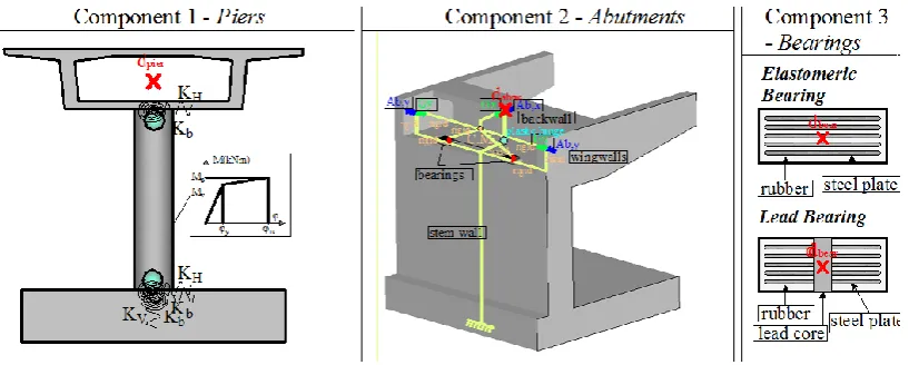
Bridge piers, abutments, and bearings (Figure 2) are considered as the critical components for the system’s seismic performance. The prestressed concrete deck is assumed to remain elastic and the pier-foundation system is considered capacity-designed, so that plastic hinges are not expected to form at the foundation level. Capacity is defined at component level, accounting for the effect of different geometric, material, loading and member detailing parameters on component strength and ductility and, eventually, damage threshold value.
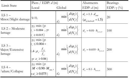
As described in [33], global engineering demand parameters are used for the quantification of component damage, accounting for different failure modes and boundary conditions. However, local to global demand parameter mapping is performed in order to describe global damage in qualitative terms. On the basis of the above, limit state (damage) thresholds for the various limit states considered in fragility analysis are defined for every component in terms of the displacement of the control point, as shown in Table 1.
Figure 2: Critical components for fragility analysis
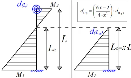
[image:5.595.88.497.496.660.2]considering different possible failure modes (flexure and shear) as depicted in Figure 3, while different boundary conditions (connection of the pier to the deck) were additionally accounted for, relating the displacement of the contraflexure point (tip of equivalent cantilever) to that at the top of the restrained pier (Figure 4). Regarding pier foundation, fixity conditions were adopted during inelastic pushover analysis for limit state threshold definition, an approach consistent with the assumption that in the common case of simplified SSI modelling, the values of linear springs calculated for shallow foundation (case of stiff soil) or pile foundation (case of soft soil) are typically high, i.e. close to fixity. It is noted that these fixity conditions refer to the threshold limit state definition in the framework of an automated procedure that permits the assessment of bridge-specific fragility. It would have been impossible to define parametrically classes of limit state thresholds accounting for all possible bridge pier geometries and properties, along with all possible SSI cases, affected by foundation configurations and soil conditions. Nevertheless, soil-structure interaction is fully taken into consideration in the holistic finite element model involving both the dynamic stiffness matrix of the abutment-embankment and the pier-foundation-subsoil boundary conditions. The effect of defining the damage thresholds for the piers using the fixed pier model was quantified for the presented case study (see section 3.3.1) and it was found that this is a legitimate simplification in the frame of the proposed procedure.
Table 1: Limit state thresholds for critical structural components
The closed-form relationship used for the estimation of limit state thresholds has the form of eq. (1) below. Parameters α1-α6 are defined on the basis of regression analysis and depend on the pier
section type (cylindrical, rectangular, hollow sections, etc.). As already mentioned, the use of the proposed relationship, ensures that the effect of different section types, as well as geometric, material, loading and reinforcement parameters on component capacity and threshold limit state values are accounted for. Threshold values calculated using eq. (1) refer to the equivalent cantilever; the level of the contraflexure point should be defined (pier top to bottom moment ratio) in order to relate them to threshold values of the restrained pier, as described in Figure 4.
1 ~ 4 exp[ 1 2 ln(D H/ ) 3 ln(v) 4 ln(fc/ fy) 5 ln( w) 6 ln( l)] Lo
(1) For the quantification of abutment and bearing damage, limit state thresholds are defined in terms of displacement of the component control point, based on experimental results and other
Limit State Piers / EDP: d (m) Abutments Bearings
Local Global EDP: d (m) EDP: γ (%)
LS 1 –
Minor/Slight damage φ1:φy
d1:
1 1 ( ) min (V ) d d
d11.1dgap
,
(backwall 1.5) 20
LS 2 – Moderate damage
φ2: min (φ:
0.004 c
, φ: 0.015 s
) d2:
2 2 ( ) min (V ) d d
2 0.01 backwall
d h 100
LS 3 –
Major/Extensive damage
φ3: min (φ:
0.004 1.4 c yw w cc f f
φ: s0.06)
d3:
3 3 ( ) min (V ) d d
3 0.035 backwall
d h 200
LS 4 –
Failure/Collapse
φ4: min (φ:
max
0.90
M M ,
φ:s 0.075) d4:
4 4 ( ) min (V ) d d
4 0.1 backwall
information from the literature, as described in [33]. In particular, threshold displacement values for abutments and bearings are related to the gap size and backwall height and shear strain, respectively (Table 1). Component capacity and limit state thresholds are defined accounting for the structure-specific parameters and properties; moreover, uncertainty in capacity (βc) and limit
state definition (βLS) should also be considered. The latter depend on component type and the
[image:7.595.220.381.268.375.2]selected demand parameter, and are quantified in [33]. Specifically, regarding bridge piers, mean and standard deviation values are assumed for key random variables, namely, material strengths, ultimate concrete strain and plastic hinge length. Latin Hypercube Sampling (LHS) is used to generate N statistically different yet nominally identical pier samples and analysis results are processed in order to calculate βc values for each limit state. For the case of bearings and abutments, the uncertainty in capacity is quantified considering the range of limit state values proposed in the literature and calculating the dispersion assuming lognormal distribution (uncertainty in limit state definition).
Figure 3: Limit state threshold on pushover curve considering both flexural and shear failure mode.
Figure 4: Top displacement of the restrained pier correlated to displacement of contraflexure point.
2.3 Earthquake ground motion selection for Incremental Dynamic and Fragility Analysis
2.3.1 Challenges
Commonly, Incremental Dynamic Analysis (IDA) [37] is used for the purposes of fragility assessment, hence, a series of nonlinear response history analyses are conducted within a wide range of the Intensity Measure (IM) adopted (typically 0≤ag≤1g for peak ground acceleration or 0≤ Sa(T1) ≤2.5g when the spectral acceleration at the fundamental period T1 is used). Ground
motion selection is therefore either based on (a) a wide, as needed, range of IM and a quite relaxed, if any, scenario of soil class, magnitude and source-to-site distance (known as M-R pair) that would permit an adequate number of eligible records, or, (b) on a bounded set of M, R and soil criteria that generally lead to a smaller sample that is inevitably appropriately scaled.
[image:7.595.189.401.409.536.2]fragility estimates as well. In the first case, (i.e., selection without scaling) it is almost impossible to form an unbiased ensemble of motions particularly in cases of higher intensity motions in softer soil profiles (for instance C or D according to Eurocode 8) as the number of available records is rather limited. The latter is due to the fact that softer soils behave nonlinearly even for small-to-moderate ground motions, thus leading to generally lower amplification factors. Often, this effectively drives the decision to the second approach (involving record scaling), which is even more subjective especially for large scaling factors [36] and potentially leads to erroneous results in both structural response [37] and soil amplification. The reason in this case is that weak motions correspond to either low magnitude - short distance, or large magnitude – long distance pairs, as well as linear elastic, or moderately inelastic soil response, hence, significant scaling generates an unrealistic set of ground motions with unrealistic frequency, waveform and duration characteristics.
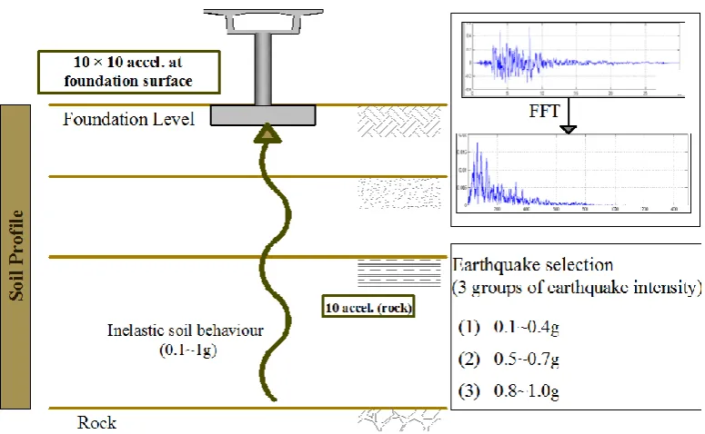
To address this issue, an alternative to the Multiple Stripe Analysis [38] is introduced, first utilising different M-R and PGA (ag) criteria for low-to-moderate, medium-to-strong and high earthquake intensities, namely:
Sub-set 1(weak to moderate motions): 0≤ag≤0.4g, M<6.5, R≤30 km
Sub-set 2 (strong, far-field, motions): 0.4<ag≤0.8g M≥6.5, R≥30km,
Sub-set 3 (very strong, near field, motions): 0.8<ag≤1.0g, M≥6.5, R≤30 km.
To further create a set of motions with unbiased representation of soil nonlinearity, the selection is performed at bedrock level (i.e., corresponding to soil A according to the Eurocode 8 classification), while a 1-Dimensional, nonlinear site response analysis is conducted to generate the foundation-exciting ground motions.
It is noted that the above procedure is applicable when the interest is in developing fragility curves for a specific bridge class in any seismic environment. In an actual case where the fragility is sought for a specific bridge in a given site, ad-hoc probabilistic seismic hazard assessment is needed. Then, given the disaggregation of seismic hazard to the Magnitude and source-to-site distance R that dominates the hazard, the appropriate ground motion sample is defined solely on the basis of the dominant M-R pair. Again, motions recorded on rock soil are to be selected as local site conditions are explicitly taken into consideration through site response analysis.
2.3.2 Ground motion selection at the bedrock level
The first edition of the earthquake NGA record database developed by PEER is used here as the seed database for the selection process [39]; it includes a total of 3557 sets of three-component earthquake records. The ground motion selection is performed in two different stages. First, a preliminary selection is made for bedrock/rock conditions (Vs30>800m/s) for each of the three
M-R pairs (herein: group 1: M≤6.5, group 2: M≥6.5, R≥30, group 3: M≥6.5, R≤30), followed by a computational search for optimum spectral matching. Herein, the divergence of the mean spectra of the selected horizontal ground motion suite from the target response spectrum is considered as the optimality criterion. The overall selection problem can then take the following mixed discrete – continuous optimization form:
2 1 1 , 1min ( , )
2
M
j j i j
N j
Tar i i
S Sa n
f Sa M
S n (2)
subject to:
max min S S
1
max nj n
where n{ }Z is the identification of each ground motion in the database space Z of the
available motions, Saj
i,n
is the spectral acceleration of the nth ground motion set from the reduced database for the Ti period, SaTar
i is the target spectral acceleration of the same periodTi, Sj is the scaling factor of each ground motion, Smin and Smax are the user-defined, minimum and maximum limits of acceptable scaling (herein set to 0.4 and 2.5, respectively) and nmax is the
Figure 5: Response spectra of the selected ground motions for Eurocode 8, Type I, Soil A target response spectrum: Sub-set 1 (0≤ag≤0.4g, M≤6.7, top left), Sub-set 2 (0.4<ag≤0.8g M≥6.5, R≥30km, top
right) and Sub-set 3 (0.8<ag≤1.0g, M≥6.5, R≤30km, bottom).
Due the governing combinatorial nature of the optimization problem, a basic search algorithm is implemented for the approximate solution of the problem with the goal criterion being the selection of the appropriate number of ground motions for each M-R pair. A greedy search algorithm is used at each domain state of the search and all possible steps are valued according to a heuristic function to select the most efficient state for expansion. The search iterates until a goal state is included in the possible steps of expansion. For this particular case, the heuristic employed for the selection of the ground motions has the following form:
2, 1 , , 1 ( ) 2 1 N
opt j i mean j i
Tar i i
S Sa n S n k
h n Sa
k
(3)where n{ }, being the reduced subspace of the available motions domain Z, Saj
i,n
is defined as previously, Smean j,
i,n
is the mean spectral acceleration for the period Ti of the sofar selected and scaled ground motions, SaTar
i is the targeted spectral acceleration for the Ti period, k is the number of the so far selected ground motions (i.e., number of states expanded so far) andSoptis the scaling factor value for which the contribution of a specific n ground motion isoptimal. As a result, for the calculation of the heuristic function of each possible step the solution (Sopt) of the following constrained quadratic optimization problem is essential, hence:
2, 1
, ,
1 min ( )
2 1
N
j i mean j i
Tar i i
S Sa n S n k
f S Sa
k
(4)again, subject to Smin S Smax. Due to the nature of the one-dimension linear constrained
quadratic optimization sub-problem, an analytical solution is accomplished by directly calculating the unconstrained optimal of the problem and projecting the solution to the bound constrains for the calculation of the heuristic value of each possible step of a state.
The Eurocode 8, Type I elastic spectrum for soil class A is used as the target spectrum for the selection optimization process, the matching being illustrated in Figure 5. Having selected 10 individual ground motions for each of the three sub-sets, limited scaling is performed within the sub-sets in order to populate the ground motion sample at an interval of 0.1g within each range (0<ag≤0.4g, 0.4<ag≤0.8g, 0.8<ag≤1.0g). This effectively resulted in the final sample of 100 ground
motions at the bedrock level (10 records of sub-set 1 × 4 intervals, plus 10 records of sub-set 2 × 4 intervals plus 10 records of sub-set 3 × 2 intervals) to be used for fragility analysis, subsequent to site response analysis.
2.3.3 Site Response
Figure 6: Generation of the earthquake ground motion ensemble
2.4 Soil-bridge interaction
2.4.1 Soil-foundation-pier interaction
The types of SSI effects considered in the proposed methodology are soil-pier foundation and embankment soil-bridge interaction, both strongly related to the frequency content of the input motion. In this regard, detailed computational procedures are implemented for ground motion selection (see §2.3), which has inevitably different frequency content but also different duration (and ability to drive soil nonlinearities) given the distinct target earthquake magnitude and source-to-site distance of the three subsets. Translational, rotational and coupled terms of the dynamic stiffness at the pier-foundation interface are derived based on analytical solutions for surface [5] or pile foundations [42] (among others) and the predominant frequency of excitation, expressed in terms of the mean frequency [43]:
2
2
1 /
i i m
i i
i C f
C f
(5)where Ci are the Fourier amplitude coefficients, fi are the discrete fast Fourier transform (FFT) frequencies between 0.25 Hz ≤ fi≤ 20 Hz and Δf ≤ 0.05 Hz is the frequency interval used in the
FFT.
2.4.2 Abutment-embankment interaction
Figure 7: Schematic representation of the proposed embankment modelling approach for: (a) longitudinal direction and (b) transverse direction
Figure 8. Simplified deck-pier-abutment substructure and embankment models [44].
The proposed analytical approach for considering bridge-embankment interaction, consists of the following steps:
Step a: Compilation of the earthquake ground motion sample (already accomplished for the entire bridge)
Step b1: Determination of the structural characteristics of the bridge (superstructure and substructure) in terms of kinematic resistances and contributing masses, assigned to the end nodes (Figure 8), to be used as boundary conditions for foundation and embankments in the analytical embankment solution of the next step (b2). The above
[image:12.595.97.504.374.568.2]is compatible with the derived deformations for the current level of earthquake intensity provided in steps b2 and b3.
Step b2: Based on the two previous steps, analytical solutions for the embankments are derived according to [7]. Embankment characteristics are provided as a function of the soil constitutive properties, as well as the frequency content of the input motion (step a) and the imposed boundary conditions (step b1). For the earthquake intensity level
considered, a convergent shear modulus value “G” is evaluated based on the recorded shear strain levels.
Step b3: A simplified structural model of the bridge is set up, wherein the embankment characteristics of the previous step are assigned to the abutment nodes utilising the aforementioned SSI elements, i.e. concentrated masses, springs, dashpots, and also gap elements to model joints.
Deformations derived using the computational model of the previous step, are used for the verification of the postulated scheme (step b1); adjustments are made wherever required; in
particular, in the usual case that derived deformations are different from the postulated ones, embankment properties are modified until convergence [15].
The embankment critical length Lc is taken equal to the wing-wall length Lwingwall. Ultimately,
the dynamic and kinematic characteristics of the embankment are evaluated for each of the selected input motion scenarios from:
c L Hc
emb B z y dz dy
M 0 0 2 * ) , ( (6)
c L H
c L H
cemb dz dy
dy y z d y z dy dz dz y z d y z B G K 0 0 2 2 0 0 2 2 * ( , ) ) , ( ) , ( ) , ( (7)
emb Bc L Hc z y dz dy
0 0 * ) , ( (8)
where *
emb
M is the embankment lumped mass attached on the deck, Kemb* is the embankment
stiffness contributions to the deck–pier–abutment substructure model, *
emb
is the generalized system excitation factor, H is the equivalent embankment height, Bcthe equivalent embankment
width, soil density and (z,y)the embankment deformation shape in both z and y axes, as defined in [15].
2.5 Seismic demand and associated uncertainties
Figure 9. Variation of PGA value between bedrock and soil surface
Statistically different, yet nominally identical bridge realizations are considered, assuming distributions and CV values proposed in [33] for selected random variables (see Table 2) and applying Latin Hypercube Sampling (LHS). Since normal distribution was adopted for material strengths, it was verified that the three-sigma rule of thumb was satisfied, hence ensuring that 99.7% of values were treated; moreover it was checked that no negative values resulted from the sampling (actually the lowest concrete strength in the LHS was 12.5 MPa). LHS is performed simultaneously on structural properties and ground motion records as described in [45] and illustrated in Figure 9. A sample size N=100 is used here, while every bridge realization is paired with the group of 10 earthquake ground motions selected, whereas 10 earthquake intensities are considered resulting in a total of 1000 analyses (100 sample size paired with 10 ground motion records x 10 intensities). Since sample size (N) is greater than the number of earthquake motions (M), records are simply recycled [45] as shown in Figure 10. Based on the results of inelastic response-history analysis for various levels of earthquake intensity, seismic demand at the control point of every component (e.g. the top of the pier) is calculated. Assuming lognormal distribution, statistical analysis of results is performed, estimating the mean and standard deviation (βd) for every critical component. Since mean and standard deviation are calculated on the basis of Monte Carlo simulation, the confidence interval (upper and lower bounds) is calculated (for the selected confidence level, i.e. 5% or 95%), based on analysis results and equation (9) (α: the confidence level, σ: standard deviation, n: sample size)
/2
: a
CI xz n
(9)
Figure 10: Estimation of uncertainty in seismic demand.
2.6 Fragility analysis of the bridge system
Using the procedure described in the previous sections, component capacity and demand, as well as probability of failure, i.e., probability that seismic demand exceeds a specific limit (damage) state threshold for various levels of earthquake intensity, are initially estimated at the component level. Assuming a series connection between components for system fragility evaluation, the damage threshold for the entire bridge is the lowest PGA value for any component. A differentiation is made in the case of the “collapse” limit state; only piers or abutments are considered to trigger the latter limit state, nevertheless the case of unseating is also considered.
System fragility curves are plotted for the limit states considered, assuming lognormal distribution. As already mentioned, mean values (threshold values in PGA terms) are calculated for each limit state and each component, whereas the system’s damage threshold is defined as the lowest component value for every limit state. Likewise, standard deviation (total uncertainty value
βtot) is initially estimated at component level based on the uncertainty in component capacity (βc), limit state definition (βLS) and seismic demand (βd), according to eq. (2) and under the simplifying
assumption of statistical independence [33].
Regarding the bridge system, the total uncertainty is related to the structural system; in particular, it is governed by pier (total) uncertainty for the case of monolithic bridge to deck connection, by bearings for simply-supported bridges and by abutments in single-span bridges. Either the same (according to the structural system) or different (according to the most critical component) βtot
value may be used for deriving the system fragility curve for each limit state, however the use of a uniform βtot value for all limit states is frequently adopted (also done herein), in order to avoid intersection of fragility curves. In this case, 2 2 2
tot c d LS
to account for all sources of uncertainty simultaneously.
3.
CASE STUDY
3.1 Overview
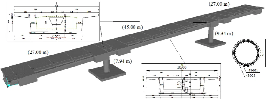
The methodology described in the previous section for deriving bridge-specific fragility curves considering SSI effects, is applied to a typical three-span overpass (T7) of Egnatia Motorway (N. Greece). The total length of the bridge is 99 m, consisting of a 45 m central span and two 27 m outer spans. The longitudinal slope of the bridge axis is constant and equal to 7% (Figure 11). The deck consists of a 10 m wide prestressed concrete box girder section, while the two piers, having a solid circular reinforced concrete section with diameter equal to 2 m, are monolithically connected to the deck. The heights of the left and the right pier are 7.9 m and 9.3 m, respectively, while two series of 48 longitudinal bars of 25 mm diameter are spaced equally around the section perimeter. The transverse reinforcement consists of an outer spiral of 14 mm diameter an inner 16 m one, both spaced at 75 mm.
Random Variable Distribution Mean CV
fc normal 28 MPa 18%
fy normal 506 MPa 8%
gap size (x/y) normal 10/15 cm 20%
Figure 11: Case study overpass (T7 Bridge)
The deck is supported on seat type abutments with a backwall height equal to 2 m, through two elastomeric bearings (350mm×450mm×136mm). Joints of 100 mm and 150 mm width separate the deck from the abutment along the longitudinal and the transverse direction, respectively. The foundation rests on surface footings given the moderately stiff soil formations corresponding to class B according to Eurocode 8. The pier footings are 9.0 m long by 8.0 m wide and 2.0 m thick, while the footings supporting the abutments are 12.0m×4.5m×1.5m. A general overview of the bridge configuration is shown in Figure 12 (bridge model). Earthquake ground motions are selected according to the optimization procedure presented in Section 2.3.2 setting the maximum permissible scaling factor to 2.0. Site response is performed assuming, for simplicity, a uniform clay profile with γ=0.022 ΜΝ/m3, soil density ρ=1.8 t/m3, undrained strength c
u=0.25 MPa, and
friction angle φ=0.
Figure 12: Geometry, pier and deck properties of case study bridge.
3.2 Alternative modelling of soil-structure interaction effects
[image:16.595.77.524.425.593.2]The embankment critical length and embankment height are both equal to 7.0 m. Furthermore, considering that boundary conditions for the embankment motion are defined by the abutments, the deformation shape was assumed as a function of height (i.e.,(z,y)(z)). Backfill-abutment and Backfill-abutment-deck gap element properties are defined according to the literature [46].
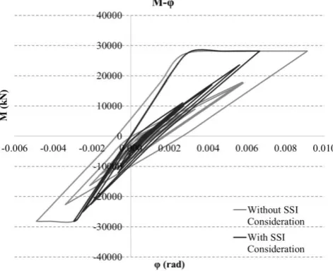
[image:17.595.70.536.201.347.2]The moment-curvature diagram of the plastic hinge at the bottom of the left pier is depicted in Figure 14, with and without the effect of soil compliance. It is noted that rocking of the pier around its base, leads to reduced curvature and seismic energy dissipation at the location of the plastic hinge.
Figure 13: Structural model of case study bridge (OpenSees) with simplified consideration of SSI (lumped linear springs).
Figure 14: Moment-curvature diagram at pier base location with and without SSI consideration (longitudinal direction)
3.3 Fragility of the bridge studied with and without SSI consideration
3.3.1 Overview
[image:17.595.179.415.405.597.2]analysis, since pier base displacement and rotation were found to be below LS1 limits as described in [47], namely 25 mm and 0.2 rad respectively.
Uncertainty in seismic demand (βd) is calculated from statistical processing of inelastic analyses results (100 sample size paired with 10 ground motion records scaled to 10 intensities), under the assumption of lognormal distribution and is quantified at both component and system level, for all variants of the bridge model, with and without SSI consideration. The total uncertainty is
calculated as 2 2 2
tot c d LS
, considering the βc values for the piers and βLS values for piers, bearings and abutments as described in [33].
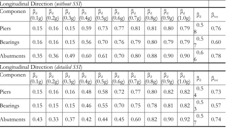
As shown in Table 3, the effect of SSI on uncertainty is minor for piers and bearings, while a slight decrease is observed in the case of abutments (mean βd values for ag 0.1~1g). However,
differences in βd values up to 21% for piers and bearings and up to 35% for abutments are
[image:18.595.65.518.290.546.2]recorded, including the uncertainty due to different modelling aspects (with and without SSI consideration) and due to record-to-record variability. Table 3 reports only the parameters for the longitudinal direction, but similar results were found for the transverse direction as well.
Table 3: Uncertainty in demand with and without SSI consideration for the longitudinal direction
Longitudinal Direction (without SSI) Componen
t
βd (0.1g)
βd (0.2g)
βd (0.3g)
βd (0.4g)
βd (0.5g)
βd (0.6g)
βd (0.7g)
βd (0.8g)
βd (0.9g)
βd
(1.0g) βd βtot
Piers 0.15 0.16 0.15 0.59 0.73 0.77 0.81 0.81 0.80 0.79 0.58 0.76
Bearings 0.16 0.16 0.15 0.56 0.70 0.76 0.79 0.80 0.79 0.79 0.57 0.60
Abutments 0.35 0.36 0.49 0.60 0.61 0.70 0.80 0.88 0.90 0.90 6 0.6 0.78 Longitudinal Direction (detailed SSI)
Componen
t (0.1g) βd (0.2g) βd (0.3g) βd (0.4g) βd (0.5g) βd (0.6g) βd (0.7g) βd (0.8g) βd (0.9g) βd (1.0g) ββd d βtot
Piers 0.15 0.16 0.16 0.48 0.58 0.72 0.77 0.80 0.82 0.82 0.54 0.73
Bearings 0.15 0.15 0.15 0.46 0.55 0.70 0.75 0.78 0.81 0.82 0.5
3 0.57
Abutments 0.43 0.33 0.37 0.42 0.44 0.45 0.60 0.82 0.90 0.92 7 0.5 0.74
The evolution of uncertainty in seismic demand values (βd) for two alternative cases, namely no
SSI and detailed SSI consideration and ag ranging from 0.1 to 1g, is depicted in figures 15 and 16,
regarding critical components and system, respectively. It is clear that both at component and system level, the uncertainty in seismic demand increases with earthquake intensity, especially for ag>0.4g. As expected, the SSI consideration affects mainly the abutment βd values, since a refined
procedure for the consideration of bridge-embankment interaction is used at this case. Finally, it should be highlighted that the detailed SSI consideration may slightly increase βd values for
Figure 15: Uncertainty in seismic demand for critical components and different levels of earthquake intensity with and without SSI consideration (longitudinal direction)
Figure 16: Uncertainty in seismic demand for bridge system and different levels of earthquake intensity with and without SSI consideration (longitudinal direction).
Bridge system and component fragilities for the limit states considered and the alternative modelling assumptions, with and without consideration of SSI effects, are depicted in Figures 17 to 21, while the limit state thresholds in PGA terms are presented in Table 4.
Table 4: Limit state thresholds [PGAxmi (g)] for the longitudinal direction, assuming three alternative boundary conditions, with and without SSI consideration.
As already mentioned in §2.2, the engineering demand parameter used for the limit state definition is the displacement of the component control point, while threshold values for LS1 to LS4 are calculated in displacement terms based on the methodology proposed for bridge-specific fragility analysis [33]. The selection of displacement as engineering demand parameter is discussed in §2.2. To assess the effect of SSI on the definition of damage states, fragility analysis considering local engineering demand parameters (namely φ and γ for piers and bearings respectively) that are not affected by SSI consideration, was additionally performed and the results regarding limit state thresholds at component and system level are presented in table 5; it is noted that the differences shown in the table do not include those that do not result from SSI (such as the effect of plastic
Limit State
Piers Bearings Abutments Bridge system
PGAxmi (g) PGAxmi (g) PGAxmi (g) PGAxmi (g)
[image:19.595.68.525.479.625.2]hinge length on transforming local curvature to pier top displacement). The differences for the case study considered are below 7% for all cases (longitudinal and transverse direction), therefore the effect of SSI consideration, namely lateral displacement and foundation rotation on limit state threshold (capacity) estimation, is low, at least for the case study considered, and can be ignored for simplicity.
Table 5: Limit state thresholds [PGAxmi (g)] considering two different engineering demand parameters (d,φ) for LS definition on component (pier) and system level.
edp : Displacement of control
point (d) edp : Curvature (φ) Difference(%)
x-direction (g) x-direction(g) x-direction (g)
C
om
po
nen
t
(P
ie
r)
F
ragil
it
y LS1 LS2 LS3 LS4 LS1 LS2 LS3 LS4 LS1 LS2 LS3 LS4
0.38 0.54 0.87 1.16 0.38 0.56 0.84 1.08 1% -4% 4% 7%
y-direction (g) y-direction(g) y-direction (g)
LS1 LS2 LS3 LS4 LS1 LS2 LS3 LS4 LS1 LS2 LS3 LS4
0.45 0.65 0.87 1.03 0.44 0.64 0.84 0.97 2% 2% 3% 6%
Sys
tem
F
ra
gi
lity LS1 LS2 x-direction (g) LS3 LS4 LS1 LS2 x-direction(g) LS3 LS4 LS1 LS2 LS3 LS4 x-direction (g)
0.18 0.54 0.86 0.94 0.18 0.56 0.85 0.93 1% -4% 1% 1% y-direction y-direction y-direction
LS1 LS2 LS3 LS4 LS1 LS2 LS3 LS4 LS1 LS2 LS3 LS4
0.21 0.65 0.73 0.89 0.21 0.64 0.75 0.87 0% 2% 3% 2%
3.3.2 Fragility at system level
[image:20.595.125.477.535.731.2]The effect of the three alternative modelling approaches (i.e., ignoring SSI, simplified SSI and refined/full SSI consideration) is compared in Figure 17 for the longitudinal and Figure 18 for the transverse direction.
Figure 18: Fragility curves for bridge system (transverse direction) assuming three alternative boundary conditions, with and without SSI consideration.
It is seen that system fragility is only marginally affected for limit states LS1-LS3. The fragility estimates in the two extreme approaches (black line for support fixity and red dotted line for refined SSI modelling) do not differ by more than 5% for LS2, while they are almost identical for LS1 and LS3 in the longitudinal direction. It is only for the collapse probability (LS4) as well as LS3 in the case of transverse direction, and for high intensities (PGA>0.5g) that the difference is substantial (up to 30%). It is also interesting to observe that, at least at system level, full consideration of embankment-bridge and soil-pier interaction systematically leads to lower probabilities of damage, irrespectively of the limit state. The intermediate model where SSI effects are only accounted for through 6-DOF springs at the base of the middle piers may provide a less conservative estimate of damage for some limit states (e.g. up to 13% compared to detailed SSI model for LS2, PGA>0.5g in the longitudinal direction). This observation highlights the dependency of fragility prediction on the modelling approach adopted, which has already been noted in the literature [48].
3.3.3 Fragility at component level
Since SSI effects may affect the hierarchy of damage between various critical components of the bridge, it is appropriate to evaluate them at component level as well, in this case piers, bearings and abutments. Component-based assessment is of particular importance when fragility analysis is performed for retrofit purposes, prior or after an earthquake event. Similarly, to Figures 17-18, Figures 19-21 illustrate the predicted fragility of the bridge piers, bearings and abutments. The observations made at system level, are also valid for the piers and bearings, as refined consideration of SSI effects reduces in general the probability of failure. This observation is, however, to some extent misleading. The reason is that, as soil compliance permits pier rocking, damage in piers is generally reduced (rigid body rotation does not inflict damage) and hence, pier fragility per se is also reduced; what is not accounted for in this case is the irreparable damage of the rocking foundation, as well as the plastic deformations of the surrounding soil, since the relevant displacement and rotation are 25mm and 0.2 rad respectively, corresponding to low damage according to [47].
A third, important, observation is that the probability of minor (LS1) and moderate (LS2) damage in the abutments is noticeably higher (up to 30%) when the embankment-bridge interaction is taken into consideration compared to the simplified approach where the abutment-embankment system is only modelled through linear springs (Figure 21). Moderate damage (LS3) and collapse (LS4) probability are not affected by SSI modelling to the same extent. Overall, assessment of bridge fragility at system level, without refined consideration of the embankment-bridge interaction may well suppress the significantly higher probability of pier foundation permanent rotation and abutment minor-to-moderate damage.
Figure 19: Fragility curves for T7 bridge piers (longitudinal direction) assuming three alternative boundary conditions, with and without SSI consideration.
[image:22.595.130.465.476.675.2]Figure 21: Fragility curves for T7 bridge abutments (longitudinal direction) assuming three alternative boundary conditions, with and without SSI consideration.
4.
CONCLUSIONS
This study presents a comprehensive framework for assessing the seismic fragility of bridges, with particular emphasis on three aspects:
(a) a more reliable (and suitable for SSI analysis) ground motion selection procedure where scaling factors are kept reasonably low (i.e., lower than 2.5), the motions are magnitude- and distance-dependent, and intensity-induced soil nonlinearities are taken into consideration through nonlinear site response analysis.
(b) the embankment-bridge interaction is explicitly taken into consideration by means of a frequency- and intensity-dependent, analytical formulation, thus significantly enhancing the reliability of the fragility assessment, and
(c) the effect of soil-structure interaction on bridge fragility is not only assessed at system level, as commonly done so far, but at component level as well, which is important, particularly in the design of retrofitting schemes.
(d) Based on fragility analysis of the case study bridge, the detailed SSI consideration results in lower probability of failure (positive effect) compared to simplified SSI consideration and fixed model at component and system level in general, except from the case of abutments, where detailed SSI consideration results in higher seismic fragility in both critical directions. The increased seismic displacements due to detailed SSI consideration together with dynamic mass participation of embankments for increased deformations, result in increased performance requirements at abutment location, for backwalls, seismic gaps and bearings. The effect of SSI consideration is more intense in the longitudinal direction since weak direction of abutment foundation is oriented towards this direction, therefore the applied boundary condition at the embankment is weak, allowing for increased embankment mass participation.
bridge piers, the associated rocking of the pier bases can be significant - however for the current case study this is not the case-.Therefore, not only fragility assessment should take SSI effects into consideration, but the assessment should take place at both system and component levels, the latter also quantitatively accounting for potential damage at the pier-foundation interface.
ACKNOWLEDGEMENTS
This research has been co-financed by the European Union (European Social Fund – ESF) and the Government of Greece through the Operational Programme “Education and Lifelong Learning” of the National Strategic Reference Framework (NSRF) – Research Funding Programme: ARISTEIA II: Reinforcement of the interdisciplinary and/or interinstitutional research and innovation and the project “Real-time Seismic Risk” (www.retis-risk.eu).
REFERENCES
[1] Mylonakis GE, Gazetas G. Seismic soil-structure interaction: beneficial or detrimental? J Earthq Eng 2000;4:277–301.
[2] Olmos BA, Roesset JM. Soil Structure Interaction Effects on. 14th World Conf. Earthq. Eng., Beijing, China: 2008.
[3] Nakhaei M, Ali Ghannad M. The effect of soil-structure interaction on damage index of buildings. Eng Struct 2008;30:1491–9. doi:10.1016/j.engstruct.2007.04.009.
[4] Kwon O, Elnashai A. The effect of material and ground motion uncertainty on the seismic vulnerability curves of RC structure. Eng Struct 2006;28:289–303.
doi:10.1016/j.engstruct.2005.07.010.
[5] Mylonakis GE, Nikolaou S, Gazetas G. Footings under seismic loading: analysis and design issues with emphasis on bridge foundations. Soil Dyn Earthq Eng 2006;26:824–53.
[6] Elgamal A, Yan L, Yang Z, Conte JP. Three-Dimensional Seismic Response of Humboldt Bay Bridge-Foundation-Ground System. J Struct Eng 2008;134:1165–76. doi:10.1061/(ASCE)0733-9445(2008)134:7(1165).
[7] Kotsoglou A, Pantazopoulou S. Bridge-Embankment Interaction under Transverse Ground Excitation. Earthq Eng Struct Dyn 2007;12:1719–40.
[8] Kappos AJ, Potikas P, Sextos AG. Seismic assessment of an overpass bridge accounting for non-linear material and soil response and varying boundary conditions. ECCOMAS Themat. Conf. Comput. Methods Struct. Dyn. Earthq. Eng. COMPDYN 2007, Rethymnon, Greece, 2007. [9] Sextos A, Mackie K, Stojadinović B, Taskari O. Simplified P-y relationships for modeling
embankment-abutment systems of typical California Bridges. 14th World Conf. Earthq. Eng., 2008.
[10] Taskari O, Sextos AG. Probabilistic assessment of abutment-embankment stiffness and
implications in the predicted performance of short bridges. J Earthq Eng 2015:150218133146008. doi:10.1080/13632469.2015.1009586.
[11] Lemnitzer A, Ahlberg E, Nigbor RL, Shamsabadi A, Wallace J, Stewart JP. Lateral performance of full-scale bridge abutment wall with granular backfill. J Geotech 2009:506–14.
[12] Shamsabadi A, Ashour M, Norris G. Bridge Abutment Nonlinear Force-Displacement-Capacity Prediction for Seismic Design. J Geotech Geoenvironmental Eng 2005;131:151–61.
doi:10.1061/(ASCE)1090-0241(2005)131:2(151).
[13] Zhang J, Makris N. Kinematic response functions and dynamic stiffnesses of bridge embankments. Earthq Eng Struct Dyn 2002;31:1933–66.
[14] Sextos AG, Pitilakis KD, Kappos AJ. Inelastic dynamic analysis of RC bridges accounting for spatial variability of ground motion, site effects and soil-structure interaction phenomena. Part 1: Methodology and analytical tools. Earthq Eng Struct Dyn 2003;32:607–27. doi:10.1002/eqe.241. [15] Kotsoglou A, Pantazopoulou S. Response simulation and seismic assessment of highway
overcrossings. Earthq Eng Struct Dyn 2009;39:991–1013. doi:10.1002/eqe.
[16] Bowers ME. Seismic Fragility Curves for a Typical Highway Bridge in Charleston, SC Considering Soil-Structure Interaction and Liquefaction Effects. Clemson University, USA, 2007.
consideration of soil structure interaction. Soil Dyn Earthq Eng 2012;40. doi:10.1016/j.neuroimage.2012.02.035.
[18] Saez E, Lopez-Caballero F, Modaressi-Farahmand-Razavi A. Effect of the inelastic dynamic soil-structure interaction on the seismic vulnerability assessment. Struct Saf 2011;33:51–63.
doi:10.1016/j.strusafe.2010.05.004.
[19] Elnashai AS, Genturk B, Kwon O-S, Hashash Y, Kim SJSJ, Jeong S-H, et al. The Maule (Chile) earthquake of February 27, 2010: Development of hazard, site specific ground motions and back-analysis of structures. Soil Dyn Earthq Eng 2012;42:229–45. doi:10.1016/j.soildyn.2012.06.010. [20] Wang Z, Dueñas-Osorio L, Padgett JE. Seismic response of a bridge–soil–foundation system
under the combined effect of vertical and horizontal ground motions. Earthq Eng Struct Dyn 2012. doi:10.1002/eqe.
[21] Ucak A, Tsopelas PC. Effect of Soil–Structure Interaction on Seismic Isolated Bridges. J Struct Eng 2008;134:1154–64. doi:10.1061/(ASCE)0733-9445(2008)134:7(1154).
[22] Zong X. Seismic Fragility Analysis for Highway Bridges with Consideration of Soil-Structure Interaction and Deterioration, Ph.D. Thesis. The City University of New York, 2015.
[23] Lesgdis N, Kwon O-S, Sextos A. Time-domain seismic SSI analysis method for inelastic bridge structures through the use of a frequency-dependent lumped parameter model. Earthq Eng Struct Dyn 2015;44:2137–56.
[24] Rovithis E, Kirtas E, Pitilakis KD. Experimental p-y loops for estimating seismic soil-pile interaction. Bull Earthq Eng 2009;7:719–36. doi:10.1007/s10518-009-9116-7.
[25] Gerolymos N, Gazetas G. Development of Winkler model for static and dynamic response of caisson foundations with soil and interface nonlinearities. Soil Dyn Earthq Eng 2006;26:363–76. doi:10.1016/j.soildyn.2005.12.002.
[26] Bayram A, Dueñas-Osorio L, Padgett JE, DesRoches R, Aygun B. Efficient Longitudinal Seismic Fragility Assessment of a Multispan Continuous Steel Bridge on Liquefiable Soils. J Bridg Eng 2011;16:93–107. doi:10.1061/(ASCE)BE.1943-5592.0000131.
[27] Wang Z, Padgett JE, Dueñas-osorio L. Influence of soil structure interaction on the fragility of an isolated bridge-soil-foundation system. 15th World Conf. Earthq. Eng., Lisbon, Portugal: 2012. [28] Mylonakis GE, Syngros C, Gazetas G, Tazoh T. The role of soil in the collapse of 18 piers of
hanshin expressway in the kobe earthquake. Earthq Eng Struct Dyn 2006;35:547–75.
[29] Fan K, Gazetas G, Kaynia AM, Kausel E, Ahmadi E. Kinematic seismic response of single piles and pile groups. J Geotech Eng Div ASCE 1991:1531–48.
[30] Kim S, Stewart JP. Kinematic Soil-Structure Interaction from Strong Motion Recordings. J Geotech Geoenvironmental Eng 2003;129:323–35.
doi:10.1061/(ASCE)1090-0241(2003)129:4(323).
[31] Mylonakis GE, Gazetas G, Nikolaou S, Chauncey A. Development of Analysis and Design Procedures for Spread Footings. Technical Report MCEER-02-0003. 2002.
[32] Gazetas G. Formulas and Charts for Impedances of Surface and Embedded Foundations. J Geotech Eng 1991;117:1363–81.
[33] Stefanidou SP, Kappos AJ. Methodology for the development of bridge- specific fragility curves, Earthquake Engineering & Structural Dynamics 2017; 46:73-93
[34] Priestley MJN, Calvi GM, Kowalsky MJ. Displacement-Based Seismic Design of Structures. IUSS Press, Pavia, Italy: 2007.
[35] Vamvatsikos D, Cornell CA. Incremental dynamic analysis. Earthq Eng Struct Dyn 2002;31:491– 514. doi:10.1002/eqe.141.
[36] Katsanos EI, Sextos AG, Manolis GD. Selection of earthquake ground motion records: A state-of-the-art review from a structural engineering perspective. Soil Dyn Earthq Eng 2010;30:157–69. doi:10.1016/j.soildyn.2009.10.005.
[37] Grigoriu M. To scale or not to scale seismic ground-acceleration records. J Eng Mech 2010:284– 93. doi:10.1061/(ASCE)EM.1943-7889.0000226.
[38] Baker JW. Trade-offs in ground motion selection techniques for collapse assessment of structures. Vienna Congr. Recent Adv. Earthq. Eng. Struct. Dyn., vol. 2013, 2013, p. 28–30.
[39] Chiou B, Darragh R, Gregor N, Silva W. NGA Project strong-motion database. Earthq Spectra 2008;24:23–44. doi:10.1193/1.2894831.
[41] Yang Z, Lu J, Elgamal A. A web-based platform for computer simulation of seismic ground response. Adv Eng Softw 2004;35:249–59. doi:10.1016/j.advengsoft.2004.03.002.
[42] Mylonakis GE, Nikolaou S, Gazetas G, Nikolaou A. Soil-pile-bridge seismic interaction: kinematic and inertial effects. part I: soft soil. Earthq Eng Struct Dyn 1997;26:337–59.
[43] Rathje EM, Abrahamson NA, Bray JD. Simplified frequency content estimates of earthquake ground motions. J Geotech Geo 1998;91:150–9.
[44] Kotsoglou A, Pantazopoulou S. Assessment and modeling of embankment participation in the seismic response of integral abutment bridges. Bull Earthq Eng 2009;7:343–61.
[45] Vamvatsikos D. Estimating Seismic Performance Uncertainty using IDA with Progressive Accelerogram-wise Latin Hypercube Sampling. Appl. Stat. Probab. Civ. Eng., 2010, p. 2704–14. [46] Nielson BG. Analytical Fragility Curves for Highway Bridges in Moderate Seismic Zones
Analytical Fragility Curves for Highway Bridges in Moderate Seismic Zones. PhD Thesis, Georgia Institute of Technology, Atlanta, 2005.
[47] Sextos AG, Kwon OS, Elnashai AS. Seismic Fragility of a Bridge on Liquefaction Susceptible Soil. ICCOSAR 2009 Int. Conf. Struct. Saf. Reliab., Osaka, Japan: n.d.
![Figure 8. Simplified deck-pier-abutment substructure and embankment models [44].](https://thumb-us.123doks.com/thumbv2/123dok_us/1431476.95700/12.595.135.464.79.322/figure-simplified-deck-pier-abutment-substructure-embankment-models.webp)