Theory blending: extended algorithmic aspects and examples

City, University of London Institutional Repository

Citation

:

Martinez, M., Abdel-Fattah, A. M. H., Krumnack, U., Gomez-Ramirez, D., Smaill,

A., Besold, T. R., Pease, A., Schmidt, M., Guhe, M. & Kuehnberger, K-U. (2017). Theory

blending: extended algorithmic aspects and examples. Annals of Mathematics and Artificial

Intelligence, 80(1), pp. 65-89. doi: 10.1007/s10472-016-9505-y

This is the accepted version of the paper.

This version of the publication may differ from the final published

version.

Permanent repository link:

http://openaccess.city.ac.uk/18663/

Link to published version

:

http://dx.doi.org/10.1007/s10472-016-9505-y

Copyright and reuse:

City Research Online aims to make research

outputs of City, University of London available to a wider audience.

Copyright and Moral Rights remain with the author(s) and/or copyright

holders. URLs from City Research Online may be freely distributed and

linked to.

(will be inserted by the editor)

Algorithmic Aspects of Theory Blending

M. Martinez · A. M. H. Abdel-Fattah ·

U. Krumnack · D. G´omez-Ram´ırez ·

A. Smaill · T. R. Besold · A. Pease ·

M. Schmidt · M. Guhe · K.-U. K ¨uhnberger

Received: July 31, 2015 / Accepted: March 22, 2016

Abstract In Cognitive Science, conceptual blending has been proposed as an impor-tant cognitive mechanism that facilitates the creation of new concepts and ideas by

Maricarmen Martinez

Department of Mathematics, Universidad de los Andes, Bogot´a E-mail: [email protected]

Ahmed Mohammed Hassan Abdel-Fattah Faculty of Science, Ain Shams University, Cairo E-mail: [email protected]

Ulf Krumnack

Institute of Cognitive Science, University of Osnabr¨uck, Osnabr¨uck E-mail: [email protected]

Danny Arlen de Jesus G ´omez-Ram´ırez

Institute of Cognitive Science, University of Osnabr¨uck, Osnabr¨uck E-mail: [email protected]

Alan Smaill

School of Informatics, University of Edinburgh, Edinburgh E-mail: [email protected]

Tarek Richard Besold

The KRDB Research Centre, Free University of Bozen-Bolzano, Bolzano E-mail: [email protected]

Alison Pease

School of Computing, University of Dundee, Dundee E-mail: [email protected]

Martin Schmidt

Institute of Cognitive Science, University of Osnabr¨uck, Osnabr¨uck E-mail: [email protected]

Marcus Guhe

School of Informatics, University of Edinburgh, Edinburgh E-mail: [email protected]

Kai-Uwe K ¨uhnberger

constrained combination of available knowledge. It thereby provides a possible theo-retical foundation for modeling high-level cognitive faculties such as the ability to un-derstand, learn, and create new concepts and theories. Quite often the development of new mathematical theories and results is based on the combination of previously in-dependent concepts, potentially even originating from distinct subareas of mathemat-ics. Conceptual blending promises to offer a framework for modeling and re-creating this form of mathematical concept invention with computational means. This paper describes a logic-based framework which allows a formal treatment of theory blend-ing (a subform of the general notion of conceptual blendblend-ing with high relevance for applications in mathematics), discusses an interactive algorithm for blending within the framework, and provides several illustrating worked examples from mathematics.

Keywords Concept Blending·Heuristic-Driven Theory Projection

1 Introduction

Conceptual blending theory (CB) [12] provides a mechanism by which novel ideas and meanings are produced by combining familiar ideas in an unfamiliar way. For instance, “trashcan basketball” integrates knowledge structures from trash disposal and conventional basketball to yield a blend: the latter is comprised of structure from each of the two domains as well as unique structure of its own [9]. The theory has gained popularity as a way of explaining high-level cognitive and linguistic phenom-ena, such as metaphor [17], analogy [3], and counterfactual reasoning [1], [18]. Even if only a few of the assumptions made about the importance of blending mechanisms within human cognition and intelligence turn out to be correct, a complete and im-plementable formalization of CB and its defining characteristics would promise to trigger significant development in artificial intelligence and any other field aiming at modeling or re-implementing capacities related to human intelligence with compu-tational means. The original approach of CB in [12], however, lacks a formal and algorithmic account.

When considering CB in mathematics, due to the axiomatized nature of mathe-matics, the most relevant form of blending is the combination of theories (as opposed to, e.g., multimodal blending of concepts and sensory modalities in arts or the blend-ing of vague lblend-inguistic concepts). Mathematical concepts are commonly understood as finitely axiomatized theories in a logical language, and combining concepts means the combination of two concept axiomatizations. This form of concept blending will consequently be referred to astheory blending.

This paper1 _{is structured as follows. In the remainder of this introduction we}

briefly survey computational approaches to CB and give a short overview of an (un-fortunately unfinished) formal account of CB developed by Goguen, and our related overall approach to theory blending. In Section 2, we introduce the formal frame-work that we use to model blending processes, and establish a notion of optimality for blends that is inspired by cognitive criteria. In Sections 3 and 4, we present an al-gorithm that, given two input theories, searches for all the optimal theory blends. We also prove the correctness and completeness of our search algorithm, and make some considerations of efficiency. As a proof of concept, we illustrate our algorithm with three worked examples in Section 5. Section 6 contrasts and discusses our method with related approaches and Section 7 finally presents our concluding remarks and our plans for future research.

1.1 Computational Accounts of Concept Blending

The earliest computational models of concept blending, [31] and [25], were based on Gentner’s structure-mapping theory (SMT) of analogy [13]. The former used seman-tic network representations of domains and the latter geneseman-tic algorithms to search the space of possible blends. Both, however, relied on handcrafted knowledge: a com-mon issue in CB models. Besold et al. [3] and [4] show how work on computational analogy models which use generalization followed by mapping (such as Heuristic-Driven Theory Projection [28]), and amalgamation (combining solutions from multi-ple cases in case-based reasoning), as opposed to SMT, can be used in blending. Other key advances include determining the fundamental characteristics of a good blend: for instance, Martins et al. [23] investigated criteria for creative concept blends, by asking participants to rate human-generated concept blends in terms of some of the optimality principles proposed in [12] and other principles connected to creativity. Confalonieri et al. provide an alternative take on the problem [8], proposing to use computational argumentation for evaluating concept blends; through an open-ended and dynamic discussion, through which meaning is constructed and blends are re-fined and improved. In a similar social context, Li et al. [19] provide a computational perspective to the notion that blending theory must take communication contexts and goals into consideration. That is, a blend may have a plurality of meanings, and can only be properly understood within the context in which it arises. Li et al. use these concepts to clarify, constrain and implement computational procedures which are ambiguous in the original non-computational theory. Many models are open to the

G

u

u

❥❥❥❥ ❥❥

)

)

❚ ❚ ❚ ❚ ❚ ❚

I1

)

)

❚ ❚ ❚ ❚ ❚

❚ I2

u

u

❥❥❥❥ ❥❥ B

Fig. 1 Goguen’s version of concept blending (cf. [14]).

criticism that the input conceptual spaces consist of handcrafted knowledge: in [30], Veale offers an alternative by introducing the notion of a conceptual mash-up, a form of blending which uses a technique Veale calls “google-milking”. This uses common questions on the web to find salient properties of a concept, which are then used to drive the blend. This follows up previous work by Veale, [29], in which he developed a CB model which automatically found its input spaces from Wikipedia and Wordnet, and used blending theory to understand novel portmanteau words such as “Feminazi” (Feminist + Nazi). Xiao and Linkola [32] have investigated blending in the context of different forms of spaces and blends: their model of multi-media blending – Visman-tic – takes in a subject and message, such as “electricity is green”, finds images for each word on flickr, and applies juxtaposition, fusion and replacement to the photos found, outputting an image which blends the two concepts. The question of what sort of spaces can be blended is considered by Kutz et al. [16], who investigate the princi-ples of blending at the level of ontologies, and show how the Ontohub/Hets ecosystem can be used to support the generation and evalution of ontological blendoids.

1.2 Goguen’s Account of CB and Our Overall Approach

An early formal account on CB, especially influential to our approach, is the classical work by Goguen using notions from algebraic specification and category theory [14]. We base our formal model, elaborated below, on Goguen’s logic-based approach. This version of CB is depicted in Figure 1, where a blend of two inputsI1andI2is

shown. Each node in the figure stands for a representation of a concept or conceptual domain as a theory, i.e., as a finite set of axioms in a formal language. We will call the nodes “spaces”, so as to avoid terms with strong semantical load such as “con-cept” or “conceptual domain”. Each arrow in the figure stands for a morphism, that is, a potentially language changing (partial) function that translates at least part of the axioms from its domain into axioms in its codomain, preserving their structure. Now, while in practice all formal languages of interest have an established semantics and the morphisms are therefore intended to act as partial interpretations of one theory into another, Goguen’s presentation of CB stays at the syntactic level, which more directly lends itself to computational treatment. The same will apply to our own ap-proach. Given input spacesI1andI2and a generalization spaceGthat encodes some

(ideally all) of the structural commonalities ofI1andI2, a blend diagram is completed

by a blend spaceBand morphisms fromI1andI2toBsuch that the diagram (weakly)

commutes. This means that if two parts ofI1andI2are translated intoBand in

A standard example of CB, discussed in [14] and linked to earlier work on compu-tational aspects of blending in cognitive linguistics (see, e.g., [31]), is that of the pos-sible blends ofHOUSEandBOATinto bothBOATHOUSEandHOUSEBOAT(as well as other less-obvious blends). Parts of the spaces ofHOUSEandBOATcan be structurally aligned (e.g. a RESIDENT LIVES-IN aHOUSE; a PASSENGER RIDES-ON aBOAT). Conceptual blends are created by combining features from the two spaces, while re-specting the constructed alignments between them. Newly created blend spaces are supposed to coexist with the original spaces: we still want to maintain the spaces of

HOUSEandBOAT.

A still unsolved question is to find criteria to establish whether a certain blend is better than other candidate blends. This question has lead to the formulation of various competing optimality principles in cognitive linguistics (cf. [12]). While sev-eral of them involve semantic aspects that escape Goguen’s and our own treatment of CB, other principles can be reasonably approached even from a more syntactic framework. For example, there is theWeb Principle(maintain as tight connections as possible between the inputs and the blend), theUnpacking Principle(one should be able to reconstruct the inputs as far as possible, given the blend), and theTopology Principle(the components of the blend should have similar relations to those that their counterparts hold in the input spaces). These three principles, taken as a pack-age, can be interpreted in terms of Figure 1 as demanding that the morphisms should preserve as much representational structure as possible. For example, one can notice that Figure 1 looks like the diagram of a pushout in category theory. Goguen actually argued against forcing the diagram of every blend to be a pushout [14], but he did claim that some forms of a pushout construction (in a 3₂-category) capture a notion of structural optimalityfor blends.

We will propose two alternative competing criteria for structural blend optimality that also work in the spirit of the Web, Unpacking, and Topology principles, and an algorithmic method for performing blending guided by those principles. We will use a framework for computational analogy making between many-sortedfirst-order theories, in order to obtain the generalization spaceG. Accordingly, our presentation in the following will be restricted to CB over first-order theories.

2 Our Framework

mapping theories belonging to different institutions [10]. In contrast to this work, our approach uses theory morphisms as a formal tool for modeling a cognitively inspired application, namely conceptual blending, in order to give a formal approach for the creative invention of new concepts in mathematics, a goal which is significantly dif-ferent from the field of specification morphisms.

2.1 Generalization Finding

Our approach is based onHeuristic-Driven Theory Projection(HDTP), which is a framework for computing analogical relations between two input spaces presented as axiomatizations in (possibly distinct) many-sorted first-order languages [28]. HDTP proceeds in two phases (Figure 2): in themapping phase, the source and target spaces are compared to find structural commonalities and a generalized space,G, is created, which subsumes the matching parts of both spaces. In thetransfer phase, unmatched knowledge in the source space can be transferred to the target space to establish new hypotheses. Our blending approach only needs the mapping phase of HDTP; the transfer phase will be replaced by a new blending algorithm in which the two inputs play a symmetric role. Accordingly, instead of talking about source and target spaces, from now on we will refer to the input spaces simply asLandR, as mnemonics for “left” and “right” in our graphical depictions of blend diagrams, but without implying any asymmetry in the role of input spaces.

Generalization (G)

s

s

❢❢❢❢❢❢ ❢❢❢❢

+

+

❳ ❳ ❳ ❳ ❳ ❳ ❳ ❳ ❳ ❳

Source (L) analogical transfer //Target (R)

Fig. 2 HDTP’s overall approach to creating analogies (cf. [28]).

During the mapping phase in HDTP, pairs of formulae fromL andR are anti-unified, resulting in a generalization theoryGthat reflects common aspects of the in-put spaces. Anti-unification [26] is a mechanism that finds least-general anti-unifiers of expressions (formulae or terms). An anti-unifier ofA andBis an expressionE such thatAandBcan be obtained fromEvia substitutions.Eis a least-general anti-unifier ofAandBif it is an anti-unifier such that the only substitutions onEthat yield anti-unifiers ofAandBact as trivial renamings of the variables inE. First-order anti-unification, where only first-order substitutions are allowed, is not powerful enough to capture structural commonalities and produce the generalizations needed in HDTP. A special form ofhigher-orderanti-unification is therefore used where, under certain conditions, relation and function symbols can also be included in the domain of sub-stitutions (see [28] for the details). The generalized theoryGcan be projected into the original spaces by higher-order substitutions which are computed by HDTP during anti-unification. In the language of theories and theory morphisms, what HDTP does can be described as follows: based on (axiomatizations of) the two input theories, a pair of (derived) signature morphismsΣL

σL ←−ΣG

σR

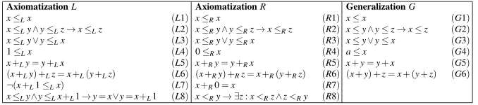
Table 1 The two axiomatizations,LandR, and the first generalizationGused in Example 1.Gcomes together with aleft substitutionλG={a7→1,≤ 7→ ≤L,+7→+L}and aright substitutionρG={a7→ 0,≤ 7→ ≤R,+7→+R}from whichLandRcan be recovered.

AxiomatizationL

x≤Lx (L1)

x≤Ly∧y≤Lz→x≤Lz (L2)

x_≤Ly∨y≤Lx (L3)

1_≤Lx (L4)

x+Ly=y+Lx (L5)

(x+Ly) +Lz=x+L(y+Lz) (L6)

¬(x+L1≤Lx) (L7) x≤Ly∧y≤Lx+L1→y=x∨y=x+L1 (L8)

AxiomatizationR

x≤Rx (R1)

x≤Ry∧y≤Rz→x≤Rz (R2)

x_≤Ry∨y≤Rx (R3)

0_≤Rx (R4)

x+Ry=y+Rx (R5)

(x+Ry) +Rz=x+R(y+Rz) (R6)

x+R0=x (R7)

x<Ry→ ∃z:x<Rz∧z<Ry (R8)

GeneralizationG

x≤x (G1)

x≤y∧y≤z→x≤z (G2)

x_≤y_∨y_≤x (G3)

a_≤x (G4)

x+y=y+x (G5)

(x+y) +z=x+ (y+z) (G6)

mapping between (combinations of) symbols of the signaturesΣL andΣR. Further-more, (axioms for) a generalized theoryGare proposed in a way that assures that

σL:G→LandσR:G→Rare theory morphisms.

It should be noted, that all processes in HDTP are syntax-based, and in its most basic form, the axioms ofLandRhave to be chosen in a way that they exhibit a par-allel structure allowing for simple matching. This is a rather strong assumption that can be found in most analogy frameworks, but which seems artificial in many practi-cal applications. In the context of HDTP, a “re-representation” mechanism has been proposed by which formulae derived from the axioms may be used in the mapping phase if the original axiomatizations do not yield a good analogical relation (cf. [28, pp. 258]). Thus, syntactically different but semantically equivalent axiomatizations may result in a good generalization. However, as this paper focuses on the blending step, we will not further consider re-representation here, i.e. we expect the axioms of the theoriesLandRto be given in a suitable form.

We will say that a formula of the input theories iscoveredbyGif it is in the image of the projection ofG; otherwise it isuncovered. Two formulae (or terms) from the input spaces that are generalized (i.e. anti-unified) to the same expression inGare considered to be analogical. In analogy making, the analogical relations are used in the transfer phase to translate uncovered facts from the source to the target space, while blending combines uncovered facts from both spaces. The blending process can thus build on the generalization and substitutions provided by the analogy engine, and analogy can be considered a special case of blending.

2.2 Optimal Blends

There are two extreme cases of CB, depending on the portion of the input theories covered byG. The first case (left side of Figure 3) occurs when the input spaces are isomorphic, meaning thatRis obtained fromLvia a renaming of symbols of the sig-nature ofLto symbols of the signature ofR. In that case, all formulae of the theories can be generalized and are completely covered byG, and the resulting blend will be isomorphic to both of them. The other extreme case (right side of Figure 3) occurs when no formulae can be aligned and therefore the generalized theoryGis empty, so no formulae of the input theories are covered. In this case, a blend can always be obtained by taking the (possibly inconsistent) disjoint union of the input theories. In practice, neither of the two extreme cases is of a real interest. The interestingproper blendsarise when only parts of the input theories are covered byG. In fact, one can adjust the blend by changing the generalization, either by removing formulae fromG and so reducing its coverage, or by choosing altogether anotherGwhich associates different formulae.

G _∼=

( ( ◗ ◗ ◗ ◗ ◗ ◗ ∼ = v v ♠♠♠♠ ♠♠ L ∼

=P((

P P P P ∼ = _// R ∼ = v v ♠♠♠♠ ♠

L∼=R

/0 ( ( P P P P P P v v ♥♥♥♥ ♥♥ L ( ( P P P P P R v v ♥♥♥♥ ♥

L⊕R

Fig. 3 The two extreme cases of input spaces, along with their generalizations and blends.

Given the generalization G, the theories L and Rcan be split into their (non-empty) covered partsL+_GandR+_Gand uncovered partsL−_GandR−_G. The covered parts are fully analogical, i.e. basically isomorphic, and make up the core of a blendBbased onG. The uncovered parts reflect the idiosyncratic aspects of the spaces, which we would ideally want to integrate intoB. However, due to the identifications induced by G, adding all this toBmay result in an inconsistent theory. To preserve consistency, we may be forced to consider only consistent subsets of this ideal, fully inclusive, blend. In view of this, we propose to define optimality of blends (see Definition 1) using the following two optimality principles:

Compression Principle (CP) aim for blend diagrams in whichBis as compressed as possible, that is, where as many signature symbols are aligned byGas possible and are actually integrated as a single symbol inB.

Informativeness Principle (IP) aim for blend diagrams in which B is as informa-tive as possible, i.e., it includes a maximally consistent subset of the potentially merged formulae (obtained by taking the union of the input theories and then col-lapsing pairs of signature symbols that have been identified by the analogy into one unified symbol).

other relations etc. Due to the fact that Fauconnier and Turner’s approach is informal and does not contain any technical details, our principles can be seen as a possible for-mal manifestation of the underlying ideas in [12]. Furthermore, different degenerated examples of (non-)compressed and (non-)informative blends can be explained using Fig. 3. Whereas a blendL⊕Ris maximally informative, because a maximal subset of the merged formulae is included (although the blend space might be inconsistent) it is nevertheless non-compressed.L∼=Ris maximally compressed and maximally informative, because all theories are essentially isomorphic. If we take for the blend in this case notLorRbut a proper subset ofL(or alternativelyR), in the extreme case the empty set, such a blend would be non-informative and non-compressed. Note fi-nally that IP renders a version of the Web and Topology principles formulated in the introduction, while CP supports the Unpacking Principle.

Definition 1. We call a blend diagramoptimalif its blend space is consistent and satisfies CP and IP. That is, if it is consistent and as maximally compressed and in-formative as possible.

2.3 Searching for Optimal Blends

Just as Figure 2 and Table 1 suggest, every generalization we use, sayH, will come in association with both a partial signature morphismλHfrom the signature ofHto

ΣL, and a partial signature morphismρH from the signature ofHtoΣR. We will use the notationH=hH,λH,ρHiwhenever we need to encode this full structure, and we will say thatHis arelaxationofG=hG,λG,ρGiifH⊆G,λH⊆λG, andρH⊆ρG.

H

t

t

❥❥❥❥ ❥❥

*

*

❚ ❚ ❚ ❚ ❚ ❚

L

*

*

❚ ❚ ❚ ❚ ❚

❚ R

t

t

❥❥❥❥ ❥❥ B

Fig. 4 An element of our search space.

With that in mind, we can now state the problem we want to solve. We take as given two first-order theoriesL andR over signatureΣL andΣR, respectively, and a generalizationGof these two theories (we have in mind a generalization found by HDTP to be as good as possible in terms of coverage). We want to find, in an algorithmic way, all the optimal blend diagrams of the form shown in Figure 4 that satisfy all of the following constraints:

1. His arelaxationofG.

2. The signatureΣBofBis a ‘right collapsed union’ ofΣLandΣR, constructed thus: add toΣBall the uncovered symbols from both input signatures, and, in addition, for each pair of symbolssL∈ΣLandsR∈ΣRthat are aligned by the generalization

H, add the symbol fromΣRtoΣB. In the last case, we say that the two symbols werecollapsedinto one.

4. Every formula inBthat is not inL+_Hmust belong toAxH=TrH(L−H)∪R−H, where TrH(L−H)is obtained fromL−H by replacing every symbol ofΣL (covered byH) by its counterpart inΣR. This ensures that all formulae ofAxH are built over the signatureΣB.

Notice that applying condition (2) above to the theories of Example 1, yields that

ΣBwill coincide withΣR, since no symbol inΣLis uncovered by the left substitution. It is tempting to conclude, also from condition (2) above, that our approach is biased towards one of the two input domains, as it always prefers choosing vocabulary from the right input space when forming blends. However, as will become clear later, the core of our algorithmic approach is unchanged if a different symbol collapsing method is used to form the signatureΣB. Alternatively, we could extend our algorithm with a final step that produces, for each discovered optimal blend, all of its “mirror” blends, obtained by alternative choices of vocabulary. This is the reason why we claim the treatment of the two input spaces is essentially symmetric.

With one more piece of notation that will also be useful later, we will be able to reformulate our search problem in a more concise way. Let B=hH,λH,ρH,Bi denote a blend diagram such as that of Figure 4. This notation does not explicitly include all the morphisms of the diagram, but only those from the generalization to the inputs, since all others are trivial to fill-in if needed (they are partial identity func-tions betweeen signatures or translafunc-tions using theTrH). Then, we want an algorithm that, givenL,RandG, will explore (in search of all the optimal blends) the space of all blend diagrams of the formB=hH,λH,ρH,Bifor which the two following conditions hold:

(i) H=hH,λH,ρHiis arelaxationof the generalizationG=hG,λG,ρGi, in the sense thatHcan be obtained fromGby dropping one or more of the renamings of symbols induced byG, so thatH⊆G,λH⊆λG,ρH⊆ρG.

(ii) R+_H⊆B_⊆R+_H∪AxH.

The above conditions can be summarized in plain language by saying that the search space (given the fixed optimal generalizationGprovided by HDTP) is the collection of all blend diagrams that are at least as informative as somehH,λH,ρH,R+Hi, where

hH,λH,ρHiis a relaxation ofG. MakingHlarger means moving in the search space towards more compressed blends, while lettingHunchanged and enlargingBmeans moving towards more informative blends.

An unconstrained way to algorithmically identify a list of optimal blends leads to an explosion of possibilities to be tried, so good heuristics are needed in order to choose which possibilities to test first (see also Section 4). Notice that for a given generalizationH, the formulae in AxH would give rise to 2|AxH| possible ways in which a subset of zero or more of the |AxH| unpaired formulae from bothL and R can be formed (and thus a way in which a blend diagram in our search space, with generalization spaceH, can be formed). Extending a generalizationHwith each of these subsets results in 2|AxH| _{corresponding sets that eventually form a network}

of theories isomorphic to the power set algebra of a set with|AxH| elements. This network can thus be represented by a lattice

L

H =h

B

B

3 Theory Blending Algorithm

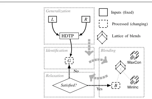
Now we are ready to present and discuss our overall search strategy, depicted in Figure 5 and further explained in the rest of this section. Given two inputsLandR over first-order signaturesΣLandΣR, respectively, we propose the following 4-stage strategy to find optimal blends.

1. Generalization: Using the HDTP mapping phase, compute a generalizationGthat is as strong as possible (i.e., identifies as many symbols as possible) together with its associated substitutions2. As an example, see Table 1 and Example 1. 2. Identification: Based on the current generalizationH⊆G(initially set toG), build

a blend signatureΣB by forming the ‘right collapsed union’ of ΣL andΣR de-scribed in the previous section.

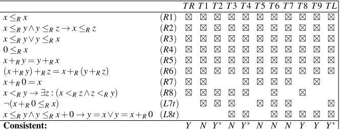
3. Blending: Construct the set of all formulae overΣBthat might be part of a blend. For a generalizationH⊆G, this will consist of every formula inR+_H(the covered part of R) plus every formula in the uncovered parts ofR and L (i.e., AxH = TrH(L−H)∪R−H). As an example, the setAxG={R7,R8,L7t,L8t}corresponds to theTrG(L−_G)

+

R−_G

=4 uncovered formulae of Example 1. These 4 formulae are listed at the bottom of the leftmost column of Table 2, which also shows the candidate blends for the particular generalizationGof that example.

ForH_⊆G, the setR+_H∪AxH∈

B

B

H ⊆B⊆R+H∪AxH. For the running example, this involves exploring the 16 theories of the lattice

L

Gdepicted in Figure 6.

The user of the algorithm decides now if the produced blends are good enough or the search must continue. In the first case we stop. If not, go to the next step which will need the setMinInc_{of minimally inconsistent subsets ofR}+

H∪AxHthat extendsR+_H.

4. Relaxation: Reduce the set of symbols covered by the current generalization by shrinking this generalization (some simple heuristics for this step are given be-low), and return to step 2.

In search of maximally informative blends, the main idea of this 4-stage general strat-egy is to scan the search space in “layers”. Each layer is determined by a generaliza-tion, starting with the fixed generalization initially given by HDTP. Then, each time the relaxation step is encountered, consequent generalizations are relaxed, meaning that the scan starts all over with a weakened relaxation (i.e., those generalizations par-tially losing their “compression”). This process of “layer scanning” corresponds to the Identification–Blending–Relaxation cycle of steps depicted visually in Figure 5.

Generalization

Identification

Relaxation

Blending

L R

G

B

HDTP

MinInc MaxCon

Satisfied?

Inputs (fixed)

Processed (changing)

Lattice of blends

Yes No

Fig. 5 A depiction of the algorithm’s overall logical flow.

3.1 Blending-Stage Algorithms

In the rest of this section, we focus on step 3 only: step 1 is obtained from HDTP, step 2 does not require further explanation, and step 4 will be discussed in Section 4. The pseudocode of step 3 comprises the procedures shown in Algorithms 1 and 2.3

Algorithm 1The COMPUTEBLENDSprocedure that is used in the blending step.

1: procedureCOMPUTEBLENDS(R_H+,AxH,Init,direction) 2: [MaxCon,MinInc] := [/0,/0]

3: for eachT∈Initdo

4: [MaxCon_,MinInc_{] = E}XPLORER+_H,AxH,T,direction,[MaxCon,MinInc] 5: end for

6: return[MaxCon,MinInc] 7: end procedure

In Algorithm 1, we have a simple procedure COMPUTEBLENDSwhich, besides

the setsR+_HandAxHintroduced above, needs a list ‘Init’ of initial blend candidates (so each element ofInit_extendsR+

H).Initmust have the property that every possible blend based on the current generalizationHis either a superset or a subset of one of the elements ofInit_{. This —plus the way in which}Init_{will be changed in the relaxation} phase (more on this below)— guarantees that the algorithm will findallthe optimal blends if never asked to stop the search (at the end of step 3). At the very beginning of the process (step 1 above)Init_{can be initialized, for example, to be the set of theories} that extendR+_G (a different choice will be used later in our worked example). When a relaxation is needed (step 4 above) a new setInit_{is computed from}MaxCon_and MinInc_{(more on this later). There is a fourth parameter (‘}direction_{’) which is used to}

direct the search (as explained soon).

3 _{A Prolog implementation of the algorithm is available athttp://www.coinvent-project.eu/en/}

The first thing the procedure COMPUTEBLENDSdoes is to initialize as empty two global setsMaxCon_andMinInc_{(lines 2 and 3 in Algorithm 1), which will keep at all} times during the search the largest consistent theories and the smallest inconsistent theories, respectively, that have been found up to the moment. After this initializa-tion, the procedure enters into a loop in which for each initial theoryT inInit_{, the} procedure EXPLORE(line 5 in Algorithm 1) will populateMaxCon_andMinInc_{. After} execution, all blends that containT or are contained in T, will be “classified cor-rectly” byMaxCon_andMinInc_{, i.e. each blend will be subsumed by some theory in} MaxCon_{if it is consistent, or will subsume some theory from}MinInc_{if it is}

incon-sistent (cf. Lemma 1 below). When the loop ends,MaxCon_{determines precisely the} optimal blends.

Algorithm 2The EXPLOREprocedure (cf. Algorithm 1).

1: procedureEXPLORE(R+_H,AxH,T,direction,[MaxCon,MinInc]) 2: ifT6∈↓MaxCon_{∪ ↑}MinIncthen

3: ifTis consistentthen

4: MaxCon_{:={T} ∪ {M∈}MaxCon_|M6⊆T}

5: else

6: MinInc_{:={T} ∪ {M∈}MinInc_|T6⊆M}

7: end if

8: end if

9: ifT∈↓MaxConand(direction_{∈ {up,both})}then

10: for eachAxiom∈(AxH\T)do

11: EXPLORER+_H,AxH,T∪ {Axiom},up

12: end for

13: else ifT∈↑MinIncand(direction_{∈ {down,both})}then

14: for eachAxiom∈T\R+Hdo

15: EXPLORER+_H,AxH,T\ {Axiom},down

16: end for

17: end if

18: return[MaxCon_,MinInc_]

19: end procedure

The EXPLOREprocedure is given in Algorithm 2, where the notations↑Cand↓C are used for a given theoryC: ↑Cdenotes the set of theories that contain some theory fromC, whereas ↓Cdenotes the set of theories that are contained in some theory fromC;lCis↑C_{∪ ↓}C. As a first step in EXPLORE(cf., lines 2 to 8 in Algorithm 2), if T is not yet classified by MaxCon _orMinInc_{, consistency of T is checked and} eitherMaxCon_orMinInc_{is updated accordingly. IfT is consistent (inconsistent), a} recursive upwards (downwards) search towards extensions (subsets) ofT is initiated. The upward and downward searches are performed unless the ‘direction_{’ parameter} prohibits them. The calls to EXPLOREmade when working with the first, strongest generalizationGuse always the direction ‘both’, with the effect that upwards and downwards searches are allowed. In the case of calls to EXPLOREafter a ‘relaxation’ has been made, the direction is set toup(the reasons for this will be explained later)4.

4 _{There are standard ways to improve the efficiency of the above procedure (using ordered lists, for}

3.2 Correctness and Completeness of the Blending Stage

The above claims about EXPLOREfollow from the next result, in whichR+_H andAxH are fixed and “theory blend” refers to setsT such thatR+_H⊆T ⊆R+_H∪AxH.

Lemma 1. The following pre- and post conditions hold true of the operation of EXPLORE R+_H,AxH,T,direction, for all theory blends T :

(1) If all consistency checks can be accomplished, the procedure will terminate. (2) IfMaxCon_andMinInc_{classify correctly before callingEXPLORE, then the same} holds afterwards.

(3) If a theory blend B is classified correctly byMaxCon_andMinInc_{before calling} EXPLORE, then the same holds after executingEXPLORE.

(4) If direction=up andMaxCon_andMinInc_{classify correctly before callingE}X

-PLORE, then ↑T is classified correctly byMaxCon_andMinInc_{after executingE}X

-PLORE.

(5) If direction=down andMaxCon andMinIncclassify correctly before calling EXPLORE, then _↓T is classified correctly by MaxCon andMinIncafter executing EXPLORE.

(6) If direction=both andMaxCon_andMinInc_{classify correctly before callingEX} -PLORE, then _lT is classified correctly byMaxCon_andMinInc_{after executingEX} -PLORE.

Proof. To show (1) notice first that the recursion will only occur with strictly larger (direction=up) or strictly smaller (direction=down) values forT. As the size ofT is limited byR+_HandR+_H∪AxHthe claim follows.

(2) follows directly, asMaxCon _{is only changed when a consistent blend}T is added. The case forMinInc_{is analogous.}

(3) LetBbe a consistent blend. By assumptionB_∈↓MaxCon_{before executing} EXPLORE.MaxCon_{is only changed if T is consistent butT 6∈}MaxCon_{, in which} caseMaxCon _{will become {T} ∪ {M∈}MaxCon_{|M6⊆T}. Now either B⊆T or} B_⊆M_∈MaxCon_{withM6⊆T. In both casesB is classified correctly by the new} MaxCon_{. A similar argument holds for}MinInc_.

(4) We proceed by induction on the cardinality ofAxH\T. IfT is inconsistent, no recursive call to EXPLOREis made. IfT _∈↑MinInc_{there is nothing to prove. If} T ∈↑/ MinInc_{, observe thatT will be added to}MinInc_{, so at the end of the procedure} ↑T will be classified correctly byMaxCon_andMinInc_{. Now, ifT is consistent and} T∈↓/ MaxCon_{, thenT will be added to}MaxCon_{. Then, for each elementAofAxH\T,} a call EXPLORE R+_H,AxH,T∪ {A},upwill be made. By inductive hypothesis, after all these calls, every ↑(T∪ {A})is classified correctly byMaxCon_andMinInc_{, and} so (sinceTis also classified correctly) ↑T is classified correctly.

(5) The argument is analogous to that for (4), now using induction on the cardi-nality ofT_\R+_H.

Table 2 The table shows some of the theories in the search space of possible blends. Maximal consistent theories are starred. FormulaeL7tandL8tresult from transferring the uncovered formulae of axiomatiza-tionL, according to generalizationG.

T R T1T2T3T4T5T6T7T8T9T L x_≤Rx (R1) ⊠ ⊠ ⊠ ⊠ ⊠ ⊠ ⊠ ⊠ ⊠ ⊠ ⊠ x_≤Ry∧y≤Rz→x≤Rz (R2) ⊠ ⊠ ⊠ ⊠ ⊠ ⊠ ⊠ ⊠ ⊠ ⊠ ⊠ x_≤Ry∨y≤Rx (R3) ⊠ ⊠ ⊠ ⊠ ⊠ ⊠ ⊠ ⊠ ⊠ ⊠ ⊠

0≤Rx (R4) ⊠ ⊠ ⊠ ⊠ ⊠ ⊠ ⊠ ⊠ ⊠ ⊠ ⊠

x+Ry=y+Rx (R5) ⊠ ⊠ ⊠ ⊠ ⊠ ⊠ ⊠ ⊠ ⊠ ⊠ ⊠

(x+Ry) +Rz=x+R(y+Rz) (R6) ⊠ ⊠ ⊠ ⊠ ⊠ ⊠ ⊠ ⊠ ⊠ ⊠ ⊠ x+R0=x (R7) ⊠ ⊠ ⊠ ⊠ ⊠ ⊠ ⊠ x<Ry→ ∃z:(x<Rz∧z<Ry) (R8) ⊠ ⊠ ⊠ ⊠ ⊠ ⊠ ⊠ ¬(x+R0≤Rx) (L7t) ⊠ ⊠ ⊠ ⊠ ⊠ ⊠ ⊠ x_≤Ry_∧y_≤Rx+0_→y=x_∨y=x+R0 (L8t) ⊠ ⊠ ⊠ ⊠ ⊠ ⊠ ⊠

Consistent: Y N Y∗ N Y∗ N N N Y Y Y∗

4 “Relaxation” Revisited

In this section, we study the relaxation stage of our approach. As our framework stands, the evaluation of blends in step 3 (i.e., “blending”) and the decision to stop or continue with a relaxation, is mandatorily an interactive step that the user decides. After a current generalizationH_⊆Ghas been dealt with, and if the relaxation step is needed, it is important to find a good weakeningKofHand a good setInit_{with which} to continue to step 2 (i.e., “identification”). In principle, the framework allows for an interactive implementation where the user decides which weakened generalization to use next, or for an implementation that uses automated heuristics, such as building a weakened generalization for which: (i) only one old symbol mapping is dropped, and (ii) the fewest number of axioms become uncovered under the new generalization. In any case, once a weakened generalizationK_⊆Hhas been fixed, the previously foundMaxCon _andMinInc_{sets are used to compute an appropriate new}Init _{set as} follows. LetTrH andTrK be the old and new translation functions. To form the set

Init_{, for eachTin}MinInc_{(and optionally for every minimal extension of}MaxCon_{) add}

toInit_{the theory that results from replacing inT every formula of the formTrH(φ)} inR−_HbyTrK(φ). This newInitis good in that every optimal blend for the weakened generalization will be an extension of one of the Init_{elements. As we will see in} this section, this is why the exploration, after some relaxation has been made, can be constrained to be upwards only.

4.1 Regarding COMPUTEBLENDSand EXPLORE

before the relaxation step is ever reached, our blending procedure consists of explor-ingSG, and Lemma 1 shows that COMPUTEBLENDSindeed finds all of the optimal blends in this subspace (with the choice of parameters with which EXPLORE is in-voked). Notice also that while restricted to stay within a subspaceSH, we cannot change compression, because the generalization is fixed, so optimal blends inSHare fully determined by maximal informativeness (i.e., maximal consistency of the last componentB). The fact that after using EXPLOREfor the first timeMaxCon_and Min-Inc_{containallthe maximal consistentB’s andallthe minimal inconsistentB’s from}

SG, respectively, follows from Lemma 1 together with the condition that upon the beginning of the procedure,Init_{must be an antichain of the power set of}AxG. That is, everyB_∈

B

To explain what happens when our procedure enters into relaxation stages, it will be convenient to picture the full search space as being composed of all the subspaces

SH, ordered according toH, so thatSH SK if and only ifK is a relaxation ofH. Notice that this entails thatK_⊆H and therefore|AxH| ≤ |AxK|. Thus, if SHSK thenSH is a smaller space (in terms of cardinality) thanSK, since these spaces are isomorphic as lattices to the power sets ofAxH andAxK, respectively. Now, assume that all the optimal blends within anSH space have been found and, even more, all of the maximal consistentB_∈

B

B

SK, whereK⊂H, and find all the optimal blends in that subspace. One way to do it would be to identify a new Init_{that is an antichain of the power set ofAxK and} proceed exactly as in the case of exploring the initialSG, in a mixed up and down direction. We will show, however, that the antichain condition onInit_{is not really} needed anymore, and the results obtained forSHallow us to construct a newInitwith the property that every optimal blend must be ‘above’ one of the elements ofInit_inSK. Thus, we will only need to focus on some “subregions” ofSK. The strategy follows from Definition 2 and Lemma 2, where we use the notation[H,B]as a shortcut for

hH,λH,ρH,Bi; an element ofSH.

Definition 2. LetK=hK,λK,ρKibe a relaxation ofH=hH,λH,ρHiand let[H,B] =

hH,λH,ρH,Bibe an element ofH. The splitting ofBunderK(denotedsplitK[H,B]) is the set of all[K,B′] =hK,λK,ρK,B′isuch that:

(i) all the elements (formulae) ofBthat keep being covered by the relaxed gen-eralizationKand all the elements ofBthat werenotoriginally covered byH

belong toB′, and

(ii) any other element ofB′must belong to(R+_H\R+_K)∪TrH(L+_H\L+_K).

So, suppose that upon relaxing fromHtoK, there is exactly one formulaϕin B∩R+_H which stops being covered byK. That is, unlike before the relaxation,ϕis not anymore a simple renaming of a formula inL+_K. Then there will be exactly four elements ofsplit_K[H,B], namely, the theories(B_{\ {}ϕ_})∪C, whereC_{⊆ {}ϕ,ϕL}and

ϕL is obtained fromϕ by changing the left signature symbols that are no longer aligned byK into their corresponding symbols in the left signature (according to

hH,λH,ρHiand[K,B]∈SK, then there is a unique element[H,B′]∈SH such that [K,B]∈split_K[H,B]. We call[H,B′]thecontractionof[K,B]underH.

Lemma 2. LetK_=hK,λK,ρKibe a relaxation ofH=hH,λH,ρHi.

1. If[K,B′]∈S_K and B′ is inconsistent, then B in the contraction[H,B]of[K,B′] underHis also inconsistent.

2. If[H,B]∈S_H, B is consistent, and[K,B′]∈split_K[H,B], then B′is also consistent.

Proof. As for(1), it is a simple observation that, if there exists a way to formally derive a contradiction fromB′using first-order logic, then there also exists a deriva-tion of a contradicderiva-tion fromB, sinceBis equivalent toB′with the addition of some equality and/or equivalence axioms of the form

∀x(f(x) =g(x))or∀x(R(x)↔T(x))

which capture the alignment (identification) of more symbols byH.

Part (2) follows from the fact that saying that[K,B′]∈split_K[H,B]is the same as saying that[H,B]is the contraction of[K,B′]underH. The contrapositive of part (1) tells us thatBbeing consistent entails thatB′is consistent as well.

Back to our blending procedure, Lemma 2 tells us that, if we are after the list of all[K,B′]∈SKthat are optimal blends (i.e., maximally informative and compressed), it will be enough for us to explore the regions ofSKthat areabove(i.e., preceed) one of the elements of the setMinInc_{Hin the informativeness order (see Equation 1).}

MinInc_H=[_{split

K[H,B]:Bminimally inconsistent inSH} (1) For ifB′is consistent butBin the contraction of[H,B]of[K,B′]was also consistent, then[K,B′]would not be maximally compressed. So,Bin the contraction of[K,B′] underHmust be inconsistent.

Now, should we want to relaxKafter being done with searching optimal blends inSK, we would like to have the list of all[K,B′]∈SK whereB′ is minimally in-consistent, to be used in that new relaxation stage. But, when canB′ be minimally inconsistent? Again, Lemma 2 gives us that ifB′is inconsistent, thenBin the con-traction of[K,B′]underHmust be inconsistent. So, same as the search for optimal blends, the search of minimally inconsistentB′sfromSK can be restricted to the re-gion of the subspaceSKformed by the blends that are more informative than at least one of the elements ofMinInc_H.

4.2 Some Considerations of Efficiency

The above remarks show that the pruning we make when fixing a (relaxed) general-izationHand exploring the associated subspaceSHis not only a pruning ofSHitself, but is simultaneously a pruning of all the relaxed spacesSK that might be potentially explored in later stages by relaxingHtoK_⊂H. Remember that the subspaces that result from relaxations are larger in size. In fact, remember that anSH is isomorphic to a power set, so the size of these spaces grows exponentially with the number of axioms that need to be “split” when doing a relaxation. So it seems wise to proceed as we currently do, that is, to start by exploring the spaceSG associated with the most compressed generalization (therefore the smaller subspace), knowing that we are pruning much larger spaces at the same time. These same ideas also justify a heuristics for choosing first, among all possible relaxations of a givenH, those that would yield the smallest size for the inducedsplitsets.

In spite of all this, the complexity, in the worst case, for exploring the initial spaceSGkeeps being very high if the task is really to findallthe optimal blends, as one can come up with examples ofAxG={ϕ1, . . .ϕ2n}such that each formula of the formVψ∈Gψ∧

V

ψ∈Cϕis consistent for each subsetCofAxGwith|C|=n, but

V ψ∈Gψ∧

V

ψ∈Dϕis inconsistent for each subsetDofAxGwith|D|=n+1. Such a case would yield a listMinInc_with (2n)!

(n!)2 elements, a quantity that is asymptotically similar to √4n

πn. This is an intrinsic problem, which of course motivates the task of trying to find heuristics for exploring the search space in a more directed way that would lead to finding the “most interesting” blends first, so that in many cases one could stop at an interesting finding and not try to complete the search for all the remaining optimal blends in the space.

Our algorithm involves testing theories in first-order logic with equality for sistency; this is well-known to be undecidable in general. In our examples the incon-sistencies will be discovered quickly5, but in more elaborate situations, a resource-bounded check for inconsistency may model reasonably well the experience of math-ematicians who can work productively with theories that are believed to be consistent and later revise their results in case an inconsistency is found. Research on Nelson Oppen methods (see [21] for a survey) reveals conditions under which the satisfiabil-ity and decidabilsatisfiabil-ity of two theories is preserved when taking their union. The basic case requires the signatures of the two theories to be disjoint, but this can sometimes be relaxed. Some of these technical results might end up being useful to our work.

5 Worked Examples

5.1 Axiomatizing Arithmetical Properties

To illustrate the algorithm and suggest at least one improvement to it, we come back to take the theories shown in Table 1. Remember thatLis based on the additive

nat-5 _{HDTP and an implementation of the blending phase module are available on request. The blending}

ural numbers (starting from 1) andR on the non-negative rational numbers. Thus, the notion of ‘number’ inLis discrete with least element 1, whereas inRit is dense with least element 0 (as the neutral element for addition). We will find all the optimal blends ofLandR. The example shows that our approach isolates just a few optimal blends among many candidates, and that the short list includes (although not exclu-sively) the ones that one would expect a mathematician to judge as most interesting.

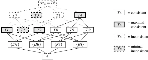
The first stage of the procedure was already partially described in the previous section. It explores the potential blends based on the generalization Gof Table 1. Figure 6 shows a lattice of the blends and Table 1 lists the axioms of each candidate blend. Our set of initial theories will be formed by the minimal extensions of theory Rand the minimal extensions of (the transferred version of) theoryL. That is,Init_:= {T1,T3,T7,T4}. The setsMaxCon_andMinInc_{are initialized as empty and we start} to explore the initial theories. The first isT1, which is inconsistent:

x+R0=x (R7)

¬(x+R0≤Rx) (L7t)

¬(x≤Rx) (Substitution)

x_≤Rx (R1)

The last two lines are clearly contradictory. The algorithm addsT1 toMinInc_. How-ever, knowing that the inconsistency arises from only the axiomsR1,R7, andL7t, it is better to add the smallerT5 toMinInc_{than addingT1 itself. Thus,}MinInc_:={T5}. Now, as the algorithm prescribes, we recursively explore (downwards) every the-ory obtained fromT1 by deleting one axiom. These theories areT R,T2, andT5:T R is consistent andT56⊆T R, soMaxCon_{:={T R};T2 is consistent, not contained in} T R, and does not extendT5, then we updateMaxCon_{:={T R,T2}; andT5 extends} the only member ofMinInc_{, so we do nothing. This ends the analysis ofT1.}

AxG=T6

T7 T3 T1 T4

T L T5 T2 T8 T9 T R

{L7t} {L8t} {R7} {R8}

/0

T x = consistent

T x = maximal

consistent

T x = inconsistent

T x = mininal

inconsistent

Fig. 6 The latticeL_B

Gof the ‘blends’ that appear in the given example.

following proof, which uses all the axioms ofT3 not covered by the generalization.

¬(x+R0≤x) (L7t)

¬(x+R0≤x)→ ∃z:(x<Rz_∧z<Rx+R0) (R8)

x<Rz_∧z<Rx+R0 (FOL)

¬(z_≤Rx)∧ ¬(x+0≤Rz) (Def.≤R)

x_≤Rz∧z≤Rx+R0 (FOL +R3)

z=x∨z=x+R0 (MP withL8t)

z_≤Rx∨x+R0≤Rx (FOL +R1 + Def.≤R)

We updateMinInc_{:={T5,T3}, and recursively explore (downwards) every theory} obtained fromT3 by erasing one axiom, namelyT L,T2, andT8:

1. T Lis consistent and does not extendT RnorT2, thenMaxCon_:={T R,T2,T L_}. We are in the “downwards” mode, so we stop.

2. T2 is a member ofMaxCon_{, so we stop.}

3. T8 is consistent and not contained in a member ofMaxCon_{. We set}MaxCon_:= {T R,T2,T L,T8}. Again, we are in the “downwards” mode, so this branch stops. This ends the analysis ofT3, the second initial theory.

The third initial theory isT7, but the analysis of it stops immediately as it ex-tendsT5∈MinInc_{. We are left with the initial theory}T4, which is consistent and not contained inMaxCon_{. Then}MaxCon_{is updated by deleting the subsets of}T4 (T R andT8) and addingT4:MaxCon_:={T4,T2,T L_}. Then we recursively explore (up-wards) for possible consistent extensions ofT4. The only proper extension ofT4 is T6, which extends elements ofMinInc_{. The first stage of the algorithm ends thus:}

– Solutions:T2,T4, andT L.

– Minimally inconsistent theories:T5 andT3.

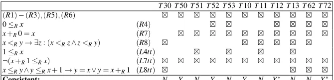
Note that T Lis just a signature renaming of theory L, T4 a case of analogi-cal transfer but not aproperblend, andT2 a proper blend intuitively describing the rationals larger than some nonzero number, which is not more interesting than the rationals starting with zero, to whichL corresponds. It is then fair to assume that the user will decide to continue the search. In the second search stage, some of the contradictions found in stage 1 will be avoided by weakening the signature of the gen-eralization in the relaxation step. The weakening heuristics described in the previous section suggest dropping the identification between 0 and 1, as this is the dropping that would diminish coverage the least. The new generalized theory changes only in that (G4) is not an axiom of it anymore. The result of transferring all of the axioms of axiomatizationLto theRside involves the introduction of a new symbol of constant (1) to theR-side; cf. Table 3.

Table 3 FormulaeLxxxresult from transferring the uncovered formulae ofLaccording to the weakened generalization that does not identify 0 and 1. Maximal consistent theories are starred.

T30T50T51T52T53T10T11T12T13T62T72

(R1)−(R3),(R5),(R6) ⊠ ⊠ ⊠ ⊠ ⊠ ⊠ ⊠ ⊠ ⊠ ⊠ ⊠

0≤Rx (R4) ⊠ ⊠ ⊠ ⊠ ⊠ ⊠

x+R0=x (R7) ⊠ ⊠ ⊠ ⊠ ⊠ ⊠ ⊠ ⊠ ⊠ ⊠

x<Ry→ ∃z:(x<Rz∧z<Ry) (R8) ⊠ ⊠ ⊠ ⊠ ⊠ ⊠

1≤Rx (L4tt) ⊠ ⊠ ⊠ ⊠

¬(x+R1≤Rx) (L7tt) ⊠ ⊠ ⊠ ⊠ ⊠ ⊠ ⊠ ⊠ ⊠ ⊠ ⊠

x_≤Ry∧y≤Rx+1→y=x∨y=x+R1 (L8tt) ⊠ ⊠ ⊠ ⊠

Consistent: N Y N Y N Y N Y∗ N N Y∗

{R4,L4tt}they contain:T j0 includes no element from{R4,L4tt},R j1 includes only L4tt,R j2 includes onlyR4, andR j3 includes the two axioms. Only some of these theories are shown in Table 3. Our set of initial theories in this stage will then be Init_{:={T30,T50}. The sets}MaxCon_andMinInc_{are reset to the empty set.}

Every maximally compressed solution blend with respect to the new generaliza-tion must extend one of the initial theories. We explore each one of these initial the-ories in the “upwards” mode. We start withT30. This theory is inconsistent because the proof used in stage 1 to see thatT3 is inconsistent still goes through when using 1 instead of 0 throughout, andL7ttinstead ofL7t. We updateMinInc_:={T30}.

Then we test the second and last initial theory, T50. The theory is consistent but may not be maximal. We updateMaxCon_:={T50}, and exploreT50’s minimal extensions:

1. T51 is inconsistent and does not extendT30, thereforeMinInc_:={T30,T51}. 2. T10 is consistent and extendsT50. SetMaxCon_{:={T10}and explore the three}

minimal extensions ofT10, thus:T60 andT11 extend the elementsT30 andT51 ofMinInc_{, so nothing is done in these cases; andT12 is consistent and properly} extendsT10. Thus, we updateMaxCon_{:={T12}and test the minimal extensions} ofT12. There are only two cases of such a minimal extension: AddingL4tt to T12 yields a theory that extends the elementT51 ofMinInc_{; and Adding L8tt} yields the theoryT62, which is inconsistent because it extendsT30∈MinInc_. 3. T70=T50∪ {L8tt} is consistent. So we update MaxCon_{:={T12,T70}, and}

explore the minimal extensions ofT70. They are:T60 (which extends T30∈ MinInc_{),T71 (which extendsT51∈}MinInc_{), andT72 (maximal consistent).} Af-ter these explorations,MaxCon_:={T12,T72}, andMinInc_:={T30,T51}. 4. T52 is a subset ofT12∈MaxCon_{, so we stop.}

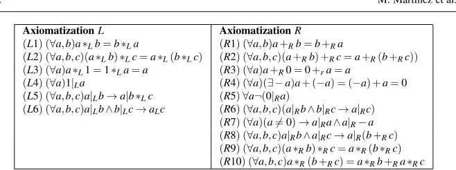
AxiomatizationL AxiomatizationR (L1) (∀a,b)a∗Lb=b∗La (R1) (∀a,b)a+Rb=b+Ra

(L2) (∀a,b,c)(a∗Lb)∗Lc=a∗L(b∗Lc) (R2) (∀a,b,c)(a+Rb) +Rc=a+R(b+Rc))

(L3) (∀a)a∗L1=1∗La=a (R3) (∀a)a+R0=0+ra=a

(L4) (∀a)1|La (R4) (∀a)(∃ −a)a+ (−a) = (−a) +a=0

(L5) (∀a,b,c)a|Lb→a|b∗Lc (R5)∀a¬(0|Ra)

(L6) (∀a,b,c)a|Lb∧b|Lc→aLc (R6) (∀a,b,c)(a|Rb∧b|Rc→a|Rc)

(R7) (∀a)(a6=0)→a|Ra∧a|R−a

(R8) (∀a,b,c)a|Rb∧a|Rc→a|R(b+Rc)

(R9) (∀a,b,c)(a∗Rb)∗Rc=a∗R(b∗Rc)

(R10) (∀a,b,c)a∗R(b+Rc) =a∗Rb+Ra∗Rc

Table 4 Explicit axiomatizations of a monoid (and a ring) with (additive) divisibility relations, respec-tively.

5.2 Commutative Ring with Unity and Compatible Divisibility Relation

We will combine two concepts emerging as a formal union of typical concepts in abstract algebra and number theory. The first conceptL is a commutative monoid with divisibility relation and the second oneRis aring with (additive) divisibility relation(compare Table 4).

We will obtain inconsistent theories in the case that all axioms ofL andRare mapped to the blend space and HDTP works with the analogical substitutions

1. ∗L→+R;|L→ |R. 2. ∗L→ ∗R;|L→ |R.

The first case is obtained when HDTP finds four direct analogical matches be-tween(L j)and(R j), for j=1,2,3,6. It is straightforward to prove that in this case 1=0, since 1 would be also a neutral element for the addition operation inR. So, the axioms (R4) and (L5) would generate a contradiction. Besides, the generic space consists of four axioms and, therefore, our algorithm suggests as a maximal con-sistent blend the concept defined by the axiomatizationRplus the axiomTrR(L5). Furthermore, the axioms(R8),(R10)andTrR(L5)imply that

(∀a,b)(a6=0)→(a|Rb).

So, a trivial model for this concept is a ring with two elements 0 and 1. In particu-lar, in this case the relation|Rbecomes almost trivial. Effectively, if we consider any ring with at least two elements, the relation|Rdefined bya|Rbif and only ifa6=0, is a model of this theory.

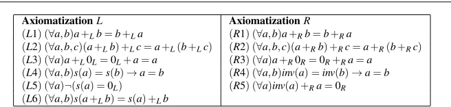
AxiomatizationL AxiomatizationR (L1) (∀a,b)a+Lb=b+La (R1) (∀a,b)a+Rb=b+Ra

(L2) (∀a,b,c)(a+Lb) +Lc=a+L(b+Lc) (R2) (∀a,b,c)(a+Rb) +Rc=a+R(b+Rc)

(L3) (∀a)a+L0L=0L+a=a (R3) (∀a)a+R0R=0R+Ra=a

(L4) (∀a,b)s(a) =s(b)→a=b (R4) (∀a,b)inv(a) =inv(b)→a=b (L5) (∀a)¬(s(a) =0L) (R5) (∀a)inv(a) +Ra=0R

(L6) (∀a,b)s(a+Lb) =s(a) +Lb

Table 5 Axiomatizations for the concepts of quasi-natural numbers as a commutative monoid with suc-cessor function (L) and Abelian group with inverse function (R).

5.3 Partial Axiomatization of the Integers

Let us consider as our first concept a partial axiomatization of the natural numbers by means of the addition operation and a successor function (see [5] for a similar axiomatization). Besides, we define as second space the concept of an Abelian group with the axioms explicitly defined through an inverse unary function (see Table 5).

In this case, HDTP finds natural analogical matches between the first four axioms of both theories, which defines the generic space. It generates the signature morphism

+L→+R; s_→inv; 0L→0R.

Our algorithm finds the blend consisting of the union of both theories as a minimal inconsistent theory. In fact, (R5) impliesinv(0R) =0R, which contradicts

TrG(L5):(∀a)¬(inv(a) =0R).

Furthermore, the set of maximal consistent theories consists basically of a space isomorphic toL and the space obtained after subtracting the former axiom, which gives the theory of Abelian groups with elements of order at most two. Effectively, the axiomsTrR(L6)and(R5)imply

(∀a)inv(a+Ra) =inv(a) +Ra=0R.

So, for any elementa=inv(inv(a)), it holds 2a=2inv(inv(a)) =0R.

In conclusion, the resulting blending gives a genuine theory with at least one new algebraic property which cannot be derived from any of the input spaces alone, namely the fact that two is an upper bound for the order of each element of the space. Now, in the interactive approach as well as in the one using automated heuristics, the next most suitable relaxation to be considered is the following one:

+L→+R; 0L→0R.

The reason is that it drops the axiom concerning the unary function symbols. So, we obtain in this case just the three first axioms of both concepts in the generic space. Again, the blended theory consisting of all the axioms inherits an equivalent kind of contradiction as in the former substitution.