Learning implicit models during target pursuit

(1)

Learning Implicit Models during Target Pursuit

Chris Gaskett

‡

_{, Peter Brown}

†1

_{, Gordon Cheng}

‡

_{, and Alexander Zelinsky}

†

†_{Robotic Systems Laboratory,Department of Systems Engineering, RSISE,}

The Australian National University, Canberra, ACT 0200 Australia

{pfb,alex}@syseng.anu.edu.au, http://www.syseng.anu.edu.au/rsl/

‡_{Department of Humanoid Robotics and Computational Neuroscience,}

ATR Computational Neuroscience Laboratories, Kyoto, Japan

{cgaskett,gordon}@atr.co.jp, http://www.cns.atr.co.jp/hrcn/

Abstract— Smooth control using an active vision head’s

verge-axis joint is performed through continuous state and ac-tion reinforcement learning. The system learns to perform vi-sual servoing based on rewards given relative to tracking per-formance. The learned controller compensates for the velocity of the target and performs lag-free pursuit of a swinging target. By comparing controllers exposed to different environments we show that the controller is predicting the motion of the target by forming an implicit model of the target’s motion. Experimental results are presented that demonstrate the advantages and dis-advantages of implicit modelling.

I. INTRODUCTION

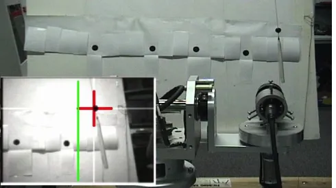
This research demonstrates learned control using one joint of a 4DOF active vision head. The task is to control the position of a target object to the centre of the robot’s field of view by reacting to the target’s movement, as shown in Fig. 1. The controller performs visual servoing—closed-loop control based on visual information—to fixate on both static and moving targets [1].

Although visual servoing does not necessarily require learning, a learning system can reduce the amount of required knowledge about the system to be controlled and reduce the reliance on calibration. A visual servoing system with learn-ing capabilities could learn to predict the movements of the target. Investigation of human vision has shown that adaption and learning improves the efficiency of gaze control [2, 3] and compensates for imperfections or changes in the eyes [4– 6]. Eye movement skills may develop incrementally during infancy [7].

Reinforcement learning is a suitable approach for learning visual servoing. Reinforcement learning systems do not re-quire an explicit dynamic model of the system to be con-trolled or a teacher to present ideal behaviour. Behaviour can be optimised over time, where the optimisation criteria is set through a reward function [8]. Our earlier research suc-cessfully applied a reinforcement learning algorithm to mo-bile robot tasks [9]. Although we were able to show that the

†_{This research was performed at the Robotic Systems Laboratory, ANU.} For a video demonstrating the results or for further information please contact Chris Gaskett.

[image:1.612.314.559.226.363.2]

1_{Department of Foreign Affairs and Trade, Canberra, Australia.}

Fig. 1. The current target-object’s position in the robot’s view (inset lower left) is marked with a red cross. The desired position is shown by a green line to the left of the cross.

robot moved smoothly, we could not confirm that the algo-rithm was predicting target movement since the robot moved slowly. Further, in the uncontrolled environment it was diffi-cult to perform comparative experiments. Performing exper-iments on an active head allowed repeated, safe experexper-iments at speeds high enough to investigate the dynamic qualities of a learned controller.

A controller with good dynamic properties would pursue moving targets smoothly with the minimum possible lag. Smooth, low-lag pursuit reduces blurring and reduces the probability of losing the target from view. Lag is introduced by delays in sensing, processing, and actuation. To minimise lag, the controller should compensate for the velocity of the target, predict the target’s movement, and be capable of pro-ducing smoothly varying actions.

II. THELEARNINGALGORITHM

In reinforcement learning tasks the learning system must

discover by trial-and-error which actions,u, are most

valu-able in particular states, x [8]. In reinforcement learning

(2)

to states is called its policy.

Evaluative feedback is provided in the form of a scalar

re-ward signal, r, that may be delayed. The reward signal is defined in relation to the task to be achieved; reward is given when the system is successfully achieving the task.

Q-Learning is a method for solving reinforcement learning

problems. Q-Learning stores the expected value, Q(x, u),

of performing each action in each state, assuming that the actions with the highest expected values will be performed thereafter:

Q(xt, ut) =E

"

rt(xt, ut, Xt+1)

+γrt+1

Xt+1,arg max ut+1

Q(Xt+1, ut+1), Xt+2

+γ2rt+2

Xt+2,arg max ut+2

Q(Xt+2, ut+2), Xt+3

+. . .

#

where probabilistic variables are capitalised; andγis the

dis-count factor, between 0 and 1, that makes rewards that are earned later exponentially less valuable. The action-values

are updated through the one-stepQ-update equation [10]:

Q(xt, ut)←−α r(xt, ut, xt+1) +γmax ut+1

Q(xt+1, ut+1)

whereαis a learning rate (or step size), between 0 and 1, that

controls convergence.

Accurate pursuit of a moving target requires continuously variable actuator commands, and the ability to respond to smooth changes in state. However, the world of discourse for most reinforcement learning algorithms is a symbolic

rep-resentation. They treat continuous variables, for example

speeds or positions, as discretised values. Discretisation does not allow smooth control and disregards important sensed in-formation.

We avoided the limitations of discrete state and action re-inforcement learning by applying our continuous state and

action Q-learning method: wire fitted neural network Q

-learning, orWFNN. The WFNN method is based on an idea

from Baird and Klopf [11]. It combines a feedforward neural network with a moving least squares approximator to

imple-mentQ-learning (see Fig. 2). All of the learned parameters

are stored in the neural network; the interpolator assists by generalising between similar actions and performing struc-tural credit assignment. The action, not only the action’s ex-pected value, is an output from the neural network. Thus the action can vary smoothly in response to smooth changes in the state. The algorithm is capable of learning and selecting actions in retime. It also supports off-policy learning, al-lowing learning from observation of other controllers.

TheWFNN algorithm is described in detail in [12], which

also includes a description of several other continuous state

and action Q-learning algorithms. Further methods are

de-scribed in [13–16]. The purpose of this paper is not

re-description of our learning algorithm; rather, it is to discuss issues that affect all reinforcement learning systems.

~_´ ut

rt+1 ~ xt+1

~ xt

/

Neural Network

(multilayer feedforward)

~ u0,q0

/

~ u1,q1

/

~ ui,qi

/

~ un,qn

/

Wire Fitter

(interpolator)

/

Q~x, ~u´

.. .. ..

/

_ _ _ _

state actions,

values

| {z } _estimate

ofQ

Fig. 2. Architecture of theWFNNlearning system

III. EXPERIMENTALPLATFORM: HYDRA

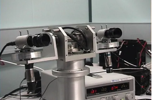
The experiments were performed on the HyDrA binocu-lar active vision platform shown in Fig. 3 [17]. HyDrA is equipped with a pair of colour NTSC cameras and has four mechanical degrees of freedom: pan, tilt, left verge-axis, and right verge-axis. The experiments reported here used only the right verge-axis and the corresponding camera. The same approach could be used for the other joints, either using one MDOF controller, or using several independent controllers. The right verge-axis controller could be transferred directly for the left verge-axis joint.

Fig. 3. The HyDrA binocular active vision head

IV. EXPERIMENTALTASK

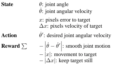
[image:2.612.320.547.63.146.2] [image:2.612.313.557.335.496.2]

(3)

State θ: joint angle

˙

θ: joint angular velocity

x: pixels error to target

∆x: pixels velocity of target Action θ˙0: desired joint angular velocity RewardP ₋

˙ θ−θ˙0

: smooth joint motion

− |x|: movement to target

[image:3.612.70.254.46.150.2]

− |∆x|: keep target still

Fig. 4. Task representation. All components are scaled by hand-crafted weighting factors.

current target was lost, the tracking process searched again over the entire view for the best matching target and selected a new current target. The learning system measured the state and produced actions at a rate of 15Hz. The low control rate exacerbates the problem of lag and, consequently, facilitates comparison of lag reduction methods.

To approach the visual servoing problem through rein-forcement learning a state, action, and reward formulation must be chosen. Figure 4 describes the representation and reward function for the fixation task. The output or action of the controller is the desired joint angular velocity. The state representation is composed of: joint position and velocity; and target position and velocity from the vision system. Joint angular velocity as returned by the HyDrA system software is a copy of the last velocity command sent; it is not measured. The joint position was included since the joint behaves differ-ently at the extremes of its range of rotation. Image velocity was estimated from the position of the target in two consecu-tive frames.

The reward is a weighted sum of negative components that punish for coarse joint motion, error in the target’s position, and target movement. Minimising the error in the target’s po-sition is the main learning task. The punishment terms are included to improve the quality of the solution by encourag-ing smooth motion.

V. RESULTS

Initially, the robot’s motions were random and the target was lost several times. User intervention was required to bring the target back into view. Within a few minutes the robot’s movements pursued the target. However, learning a controller that was competent at both pursuing moving targets and fixating on static targets was difficult. The controller was always competent at some parts of the task, but not others. More consistent results were obtained by dividing the task be-tween two controllers: the first specialising in step movement to a target (the static-trained controller), the second special-ising in smooth pursuit (the swing-trained controller). Eval-uating both of these controllers with both tasks helped us to understand why achieving competence at both tasks simulta-neously was difficult.

0 0.5 1 1.5 2 2.5 3

−25 −20 −15 −10 −5 0 5 10 15

Time (seconds)

Position (degrees, or pixels/20)

Velocity (degrees/sec, or pixels/20/sec)

[image:3.612.311.558.49.242.2]

Target Position Target Velocity Joint Position Joint Action

Fig. 5. Results from the static-trained controller pursuing a static target. The joint action is the un-filtered output from the learned controller. The target data is the error in the target object’s position and velocity based on image data in pixels, approximately scaled to the same degrees and degrees per second units as the joint data.

A. Training with Static Targets—

Evaluating with Static Targets

The static targets were the hand-held target and the targets fixed to the backing-board. The controller learnt to reliably fixate to the static targets in both directions within a few min-utes. A graph of the response showing fixation to a newly selected target is shown in Fig. 5.

Smoothness of joint motion was varied by adjusting the weighting of the smooth joint motion and pixels velocity of

target coarseness penalties in the reward function (see Fig. 4).

With appropriate coarseness penalties, the commanded ac-tion changed smoothly in response to the step change in target position. This is unlike the behaviour of a simple PID fam-ily controller and shows that the learned controller took the cost of acceleration into account. The learned controller ac-celerated more quickly than it deac-celerated, unlike HyDrA’s existing trapezoidal profile motion (TPM) controller [17].

The TPM controller accelerated with fixed acceleration to a maximum ceiling velocity, coasted at that velocity, then decelerated at a fixed rate equal to the acceleration rate. The learned controller’s strategy of accelerating more quickly seems practical since final positioning accuracy is more dependent on the deceleration phase than the accelera-tion phase. Large saccadic moaccelera-tions in humans also accelerate more quickly than they decelerate [6].

B. Training with Static Targets—

Evaluating with Swinging Targets

(4)

0 2 4 6 8 10 12 14 16 18 20 −15

−10 −5 0 5 10 15

Time (seconds)

Target Position Joint Position

Calculated Best Joint Position

10 10.5 11 11.5 12 12.5 13 13.5 14 14.5 15

−15 −10 −5 0 5 10 15

Time (seconds)

Fig. 6. Position data from the static-trained controller following a swinging target. The ideal target position is 0, the centre of the field of view.

0 2 4 6 8 10 12 14 16 18 20

−30 −20 −10 0 10 20 30

Time (seconds)

[image:4.612.309.558.49.468.2]

Joint Action Target Velocity

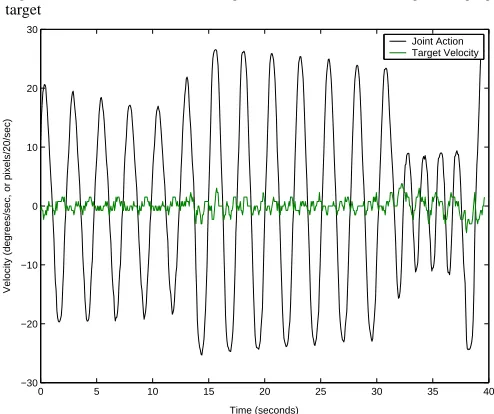
Fig. 7. Velocity data from the static-trained controller following a swinging target. The ideal target velocity is 0, i.e. the target’s position is stationary in the field of view.

0 5 10 15 20 25 30 35 40

−15 −10 −5 0 5 10 15

Time (seconds)

30 30.5 31 31.5 32 32.5 33 33.5 34 34.5 35

−15 −10 −5 0 5 10 15

Time (seconds)

[image:4.612.41.286.53.462.2]

Fig. 8. Position data from the swing-trained controller following a swinging target

0 5 10 15 20 25 30 35 40

−30 −20 −10 0 10 20 30

Time (seconds)

Joint Action Target Velocity

[image:4.612.310.557.480.687.2] [image:4.612.41.287.492.689.2]

(5)

When attempting to follow smoothly moving targets there was some lag. Lag is inevitable due to sensing and actuation delays unless the controller can predict the movement of the target. Figure 6 shows that the positioning error is highest at the bottom of the swinging motion, when the target’s veloc-ity is highest. Ideally the target position and velocveloc-ity should be maintained at zero. Using our controller there was some variance in the target position and velocity but the bias was small.

C. Training with Swinging Targets—

Evaluating with Swinging Targets

When trained only with swinging targets the controller learnt to smoothly follow the target with excellent perfor-mance within a few minutes. Figures 8 and 9 show that the swing-trained controller eliminated the pursuit lag that was seen with the static-trained controller. The swing-trained con-troller had small target velocity bias, target velocity variance, and target position variance. However, there was some bias in the target position; the bias was largest when the target was swung at a higher than normal velocity in a different position. At all times the target velocity bias and variance remained small.

D. Training with Swinging Targets—

Evaluating with Static Targets

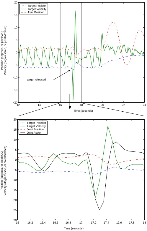
Figure 10 shows the swing-trained controller’s behaviour when exposed to a static target. Learning was again disabled so that the controller must perform the task based only its ex-perience with swinging targets. The target was held static to the left for 17 seconds. During that time the active head failed to purse the target and was nearly static. When the swinging target was released the controller successfully pursued the tar-get. The behaviour was repeatable across training sessions.

The controller rotated the camera towards the right during the first swing, matching the target velocity rather than imme-diately eliminating the target position bias. The target posi-tion bias was eliminated when the target was about to swing back. The graph shows that the joint was wiggling slightly while the target was static. The large downward spike in tar-get velocity was due to the release of the tartar-get. The lower (zoomed) portion of the graph shows that the controller was not responding to the change in target position as the target was released; it was responding to the velocity of the target. The upward spike in target velocity was due to an overshoot in the joint velocity as the controller matched the velocity of the target.

Another unexpected behaviour sometimes occurred when a pursued swinging target was seized near the extreme of its swing. The controller did not fixate the camera consistently on the now still target: it moved the joint back a few de-grees towards the central position, stopped, moved to fixate on the target again, stopped, then repeated the process. Some-times the controller made several of the ticking motions then

12 14 16 18 20 22 24

−20 −15 −10 −5 0 5 10 15 20

Target Position Target Velocity Joint Position

Time (seconds)

target released

16 16.2 16.4 16.6 16.8 17 17.2 17.4 17.6 17.8 18 −30

−25 −20 −15 −10 −5 0 5 10 15 20

Time (seconds) Target Position

Target Velocity Joint Position Joint Action

Fig. 10. Swing-trained controller failing to pursue a stationary target

stopped, fixated on the target. On other occasions the tick-ing motion was repeated, interspersed by pauses of variable length, until the target was released.

VI. DISCUSSION

Although the static-trained and swing-trained controllers had the same initial conditions, the learned controllers dif-fered because the controllers were exposed to different expe-riences. This resulted in qualitatively different behaviour. The difference was emphasised when the controllers were applied to tasks other than their speciality.

The static-trained controller did not accurately compensate for the velocity of swinging targets and lagged somewhat. Further, the bias in the target position was small, indicating that the static-trained controller responds strongly to the tar-get position.

The behaviour of the swing-trained controller when ex-posed to static targets is strong evidence that the controller

[image:5.612.310.559.50.439.2]

(6)

target the controller acted as if it was expecting swinging behaviour—waiting for the target to swing towards the mid-dle, and moving in expectation that the target will swing to-wards the middle. Prediction of target behaviour also ex-plains the zero-lag tracking performed by the swing-trained controller when exposed to swinging targets.

To verify the theory, we compared the actions of the control system to the dynamics of a pendulum model. The pendulum model was developed based on measurement of the weight of the target hanging on the string, the length of the string, and the gravitational constant. Incorporating the approximate relationship between the robot’s joint angle and the angle of the string gives the required joint acceleration to match target acceleration due to gravity2_:

¨

β= βg

l

s

1− _βd

l

2

(1)

Comparison of the model to the behaviour of the con-troller does not necessarily require analysis of experimental data gathered using the robot. It is not possible to investigate the controller’s behaviour over multiple time steps without a dynamic model of the environment, but the controller’s be-haviour over a single time step can be extracted directly from the controller itself by providing an appropriate state input. In this case the state vector has joint velocity, target position, and target velocity of zero. The joint position is the indepen-dent variable; the depenindepen-dent variable is the joint acceleration, which is calculated from the initial joint velocity and output joint velocity. Figure 11 shows joint acceleration for various joint positions. It compares the output of the swing-trained and static-trained controllers with the pendulum model and

a static object model (β¨ = 0radians/s2_{). The output from}

the swing-trained controller resembles the pendulum model, while the output from the static-trained controller is similar to the static model. This evidence supports the theory that the controllers are predicting the behaviour of the target.

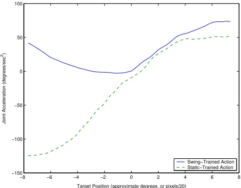
We validated the theory further by investigating the situa-tion in which a new, static target has just appeared. In this case the state vector has joint velocity, joint position, and target velocity set to zero. The target position is the inde-pendent variable. As before, the deinde-pendent variable is the joint acceleration. Figure 12 shows the output from the static-trained and swing-static-trained controllers. The static-static-trained con-troller moves in the direction of the target. The swing-trained controller moves inconsistently: if the target is to the right it moves towards the target, but if the target is to the left it moves away! The result shows that the swing-trained con-troller was specialised towards pursuing swinging targets and was not capable of fixating to static targets.

2_{Equation (1) is an approximation, and based on rough measurements of} the pendulum string length and the distance from the camera to the target at rest. The variables areβ¨radians/s2_{, the joint acceleration to match target} acceleration; andβradians, the joint angle to match pendulum angle. The constants areg= 9.81m/s2_{, the acceleration due to gravity;}_l_{= 1}_.₆_{m, the} length of the pendulum string; andd= 0.64m, the distance from the camera to target at rest.

−15 −10 −5 0 5 10 15

−100 −50 0 50 100 150

Swing−Trained Action Static−Trained Action Pendulum Model Prediction Static Model Prediction

Joint Acceleration (degrees/sec

2)

[image:6.612.310.557.50.245.2]

Joint Position (degrees)

Fig. 11. Actual output and model-predicted joint acceleration for both the static-trained and swing-trained controllers. Joint velocity, target position, and target velocity are zero.

−8 −6 −4 −2 0 2 4 6 8

−150 −100 −50 0 50 100

Target Position (approximate degrees, or pixels/20)

Joint Acceleration (degrees/sec

2)

Swing−Trained Action Static−Trained Action

Fig. 12. Joint acceleration for both the static-trained and swing-trained controllers when exposed to a static change in target position. Joint position, joint velocity, and target velocity are zero.

The WFNN algorithm does not represent the target’s

be-haviour or the dynamics of the active-head mechanism ex-plicitly. An explicit model would be a specific part of the sys-tem that can be identified as a model of the target’s behaviour,

or a model of the active-head dynamics. Rather,Q-learning

systems represent behaviour and dynamics implicitly through the stored action-values; reinforcement learning systems are known as model-free.

[image:6.612.311.558.295.488.2]

(7)

its environment, in which much of the relevant state informa-tion is unmeasured and not represented by the state vector.

However, theQ-learning algorithm assumes interaction with

a Markov environment, that is, the probability distribution of the next-state is affected only by the execution of the action in the current, measured state.

Consequently, the swing-trained controller learnt to predict the acceleration of the swinging target based on the joint po-sition (Fig. 11). Inclusion of the joint popo-sition in the state information was necessary since the joint behaves differently at the extremes of its rotation range. Nevertheless, predicting target behaviour based on joint position is obviously flawed since the model is no longer applicable if the position of the pendulum’s anchor changes (i.e. the position at rest changes). Learning a controller is competent both issuing swinging tar-gets and static tartar-gets was difficult because the learning sys-tem confounds the movement of the target with its joint move-ment. This illustrates a flaw in the model-free learning system paradigm: failing to separate controllable mechanisms from uncontrollable environment can lead to learning a controller that is fragile with respect to the behaviour of the environ-ment.

The results could be dismissed as merely another example of over-fitting, except that the type of over-fitting is highly specific, and occurs due to confounding controllable mech-anisms with the uncontrollable environment. Avoiding the problem requires a method of specifying, or learning, the dis-tinction.

VII. RELATEDWORK

Several other controllers for active heads have included ex-plicit mechanisms for coping with delays by modelling their effect and attempting to compensate [18–21]. Shibata and Schaal’s [22] active head controller had an explicit module for learning target behaviour that was capable of adapting to patterns in target movement in only a few seconds.

Human eye movements demonstrate a range of mecha-nisms for minimising lag. Basic human eye movements in-clude saccades, smooth pursuit, vergence, and the

vestibular-ocular reflexes [23]. In general, the purpose of these

move-ments is to allow the gaze to fixate on a particular object. Sac-cades are jerky eye movements that are generated by a change of focus of attention [6]. During these fast eye movements the target is not visible, making saccades an open-loop mech-anism. Saccades are based on both position and velocity so that the saccade can compensate for the expected movement of the target. Estimating the target velocity before the sac-cade is generated also allows smooth pursuit to commence immediately at approximately the correct velocity [24]. Mur-ray et al. [21] demonstrated this capability for a non-learning active head.

Smooth pursuit movements follow moving objects and keep them in the centre of the field of view [25]. The eye movement is driven by the velocity of the object, not its po-sition [26]. Popo-sitional errors are corrected through saccades. Smooth pursuit is closed-loop, predictive and adaptive [2].

Velocity of the target is an important part of the human gaze control system and non-learning mechanical active and con-trollers. Yet, many learning active head controllers do not use velocity information—they can not make a different decision based on whether the target is swinging towards the centre of the view or away.

For example, Berthouze et al. [27] smooth pursuit con-troller, based on Feedback Error Learning (FEL) [28], did not use velocity of the target. Also, current artificial ocular-motor map techniques for saccadic motion have not considered tar-get velocity [29–32]. Researchers at the LiraLab developed an integrated system, combining various biologically inspired eye and head movement mechanisms [33]. Target velocity was not considered, except when compensating for induced pan movements [34].

Shibata and Schaal’s [18] controller included velocity com-ponents as well as position comcom-ponents, based on a model of the human vestibulo-ocular reflex (VOR) and optokinetic re-flex (OKR). The VOR model included a learning component, using FEL with an eligibility trace mechanism [35].

Reinforcement learning was applied to active head control by Piater et al. [36]. The system controlled one degree of free-dom, vergence movements, in which both eyes turn inward or outward to look at an object at a particular distance [37]. Five discrete actions were available: changes in vergence angle between 0.1 and 5 degrees. The direction of the change was hard-wired. States were also represented discretely, including the positioning error. The discrete state and action representa-tion without generalisarepresenta-tion is ill-suited for this task. Vergence motions were made using discrete actions in a few steps; in contrast, human vergence motions are smooth and closed-loop [37]. The lack of generalisation in the state and action representations requires exploration of every possible repre-sentable state and action. The pure-delayed reward signal was the negative of the final positioning error. Given that this error signal is available at all times a delayed reward statement of the problem would probably result in faster learning. Piater et al.’s work appears to be the only application of reinforce-ment learning to active head control.

VIII. CONCLUSION

Continuous state and action reinforcement learning was successfully applied to control of an active head. The learned controller generated precise, smoothly varying actions. Fur-ther, the system considered the velocity of the target and per-formed lag-free tracking of a swinging target. This was possi-ble through implicitly predicting the target’s behaviour. Rein-forcement learning’s ability to optimise behaviour over time helps to compensate for sensing delays.

(8)

fragile with respect to changes in the target’s behaviour. The model-free approach is the source of the fragility: it makes no distinction between controllable mechanisms and uncontrol-lable environment.

ACKNOWLEDGEMENTS

We thank the anonymous reviewers for their comments, Dr. Thomas Brinsmead for assistance with the pendulum model, and Leanne Matuszyk and Orson Sutherland for introducing us to HyDrA.

REFERENCES

[1] S. Hutchinson, G. D. Hager, and P. I. Corke, “A tutorial on visual servo control,” IEEE Transactions on Robotics and

Au-tomation, vol. 12(5):pp. 651–670, 1996.

[2] R. J¨urgens, A. W. KornHuber, and W. Becker, “Prediction and strategy in human smooth pursuit eye movements,” in G. L¨uer, U. Lass, and J. Shallo-Hoffman, eds., Eye

Move-ment Research: Physiological and Psychological Aspects, C.

J. Hogrefe, G¨ottingen, Germany, 1988.

[3] D. L. Zhao, A. G. Lasker, and D. A. Robinson, “Interactions of simultaneous saccadic and pursuit prediction,” in Proc. of

Contemporary Ocular Motor and Vestibular Research: A Trib-ute to David A. Robinson, pp. 171–180, 1993.

[4] R. J. Leigh and D. S. Zee, “Oculomotor disorders,” in [23]. [5] H. Collewijn, A. J. Martins, and R. M. Steinman,

“Compen-satory eye movements during active and passive head move-ments: Fast adaption to changes in visual magnification,”

Jour-nal of Physiology, vol. 340:pp. 259–286, 1983.

[6] W. Becker, “Saccades,” in [23].

[7] R. N. Aslin, “Development of smooth pursuit in human in-fants,” in Proc. of the Last Whole Earth Eye Movement

Con-ference, Florida, 1981.

[8] R. S. Sutton and A. G. Barto, Reinforcement Learning: An

Introduction, Bradford Books, MIT, 1998.

[9] C. Gaskett, L. Fletcher, and A. Zelinsky, “Reinforcement learn-ing for a vision based mobile robot,” in Proc. of the IEEE/RSJ

International Conference on Intelligent Robots and Systems (IROS2000), Takamatsu, Japan, 2000.

[10] C. J. C. H. Watkins and P. Dayan, “Technical note: Q learning,”

Machine Learning, vol. 8(3/4):pp. 279–292, 1992.

[11] L. C. Baird and A. H. Klopf, “Reinforcement learning with high-dimensional, continuous actions,” Tech. Rep. WL-TR-93-1147, Wright Laboratory, 1993.

[12] C. Gaskett, D. Wettergreen, and A. Zelinsky, “Q-learning in continuous state and action spaces,” in Proc. of the 12th

Aus-tralian Joint Conference on Artificial Intelligence, Sydney,

Australia, 1999.

[13] F. Saito and T. Fukuda, “Learning architecture for real robot systems—extension of connectionist Q-learning for continu-ous robot control domain,” in Proc. of the International

Con-ference on Robotics and Automation (IROS’94), pp. 27–32,

1994.

[14] Y. Takahashi, M. Takeda, and M. Asada, “Continuous val-ued Q-learning for vision-guided behavior,” in Proc. of

the IEEE/SICE/RSJ International Conference on Multisensor Fusion and Integration for Intelligent Systems, 1999.

[15] F. Maire, “Bicephal reinforcement learning,” in Proc. of the 7th

International Conference on Neural Information Processing (ICONIP-2000), Taejon, Korea, 2000.

[16] W. D. Smart and L. P. Kaelbling, “Practical reinforcement learning in continuous spaces,” in Proc. of the 17th

Interna-tional Conference on Machine Learning, 2000.

[17] O. Sutherland, S. Rougeaux, S. Abdallah, and A. Zelinsky, “Tracking with hybrid-drive active vision,” in Proc. of the

Aus-tralian Conference on Robotics and Automation (ACRA2000),

Melbourne, Australia, 2000.

[18] T. Shibata and S. Schaal, “Biomimetic gaze stabilization based on feedback-error learning with nonparametric regression net-works,” Neural Networks, vol. 14(2), 2001.

[19] C. Brown, “Gaze controls with interactions and delays,” IEEE

Transactions on Systems, Man, and Cybernetics, vol. 20(1):pp.

518–527, 1990.

[20] D. W. Murray, F. Du, P. F. McLauchlan, I. D. Reid, P. M. Sharkey, and J. M. Brady, “Design of stereo heads,” in A. Blake and A. Yuille, eds., Active Vision, MIT Press, 1992.

[21] D. W. Murray, K. J. Bradshaw, P. F. McLauchlan, I. D. Reid, and P. M. Sharkey, “Driving saccade to pursuit us-ing image motion,” International Journal of Computer Vision, vol. 16(3):pp. 205–228, 1995.

[22] T. Shibata and S. Schaal, “Biomimetic smooth pursuit based on fast learning of the target dynamics,” in Proc. of the IEEE

International Conference on Intelligent Robots and Systems (IROS2001), 2001.

[23] R. H. S. Carpenter, ed., Eye Movements, vol. 8 of Vision and

Visual Dysfunction, Macmillan, 1991.

[24] A. L. Yarbus, Eye Movements and Vision, Plenum Press, New York, 1967.

[25] J. Pola and H. J. Wyatt, “Smooth pursuit: Response character-istics, stimuli and mechanisms,” in [23].

[26] C. Rashbass, “The relationship between saccadic and smooth tracking eye movements,” Journal of Physiology, vol. 159:pp. 338–362, 1961.

[27] L. Berthouze, S. Rougeaux, Y. Kuniyoshi, and F. Chavand, “A learning stereo-head control system,” in Proc. of the World

Au-tomation Congress/International Symposium on Robotics and Manufacturing, France, 1996.

[28] M. Kawato, K. Furawaka, and R. Suzuki, “A hierarchical neu-ral network model for the control and learning of voluntary movements,” Biological Cybernetics, 1987.

[29] H. Ritter, T. Martinetz, and K. Schulten, Neural Computation

and Self-Organizing Maps: An Introduction, Addison Wesley,

1992.

[30] R. P. Rao and D. H. Ballard, “Learning saccadic eye move-ments using multiscale spatial filters,” in Proc. of Advances in

Neural Information Processing Systems 7 (NIPS94), 1994.

[31] M. Marjanovi´c, B. Scassellati, and M. Williamson, “Self-taught visually guided pointing for a humanoid robot,” in

Proc. of the Fourth International Conference on Simulation of Adaptive Behavior, MA, 1996.

[32] M. Pagel, E. Ma¨el, and C. von der Malsburg, “Self calibration of the fixation movement of a stereo camera head,” Machine

Learning, vol. 31(1-3):pp. 169–186, 1998.

[33] G. Metta, F. Panerai, R. Manzotti, and G. Sandini, “Babybot: an artificial developing robotic agent,” in Proc. of From

Ani-mals to Animats: Sixth International Conference on the Simu-lation of Adaptive Behavior (SAB 2000), Paris, 2000.

[34] F. Panerai, G. Metta, and G.Sandini, “Learning VOR-like sta-bilization reflexes in robots,” in Proc. of the 8th European

Sym-posium on Artificial Neural Networks (ESANN 2000), Bruges,

Belgium, 2000.

[35] A. G. Barto, R. S. Sutton, and C. W. Anderson, “Neuronlike adaptive elements that can solve difficult learning control prob-lems,” IEEE Transactions on systems, man and cybernetics, vol. SMC-13:pp. 834–846, 1983.

[36] J. H. Piater, R. A. Grupen, and K. Ramamritham, “Learning real-time stereo vergence control,” in Proc. of the 14th

Inter-national Symposium on Intelligent Control (ISIC ’99), 1999.