Development of Methodologies for the Solution of the Forward Problem in Magnetic-Field Tomography (MFT) Based on Magnetoencephalography (MEG)

(1)

City, University of London Institutional Repository

Citation

:

Aristovich, Kirill (2011). Development of Methodologies for the Solution of the

Forward Problem in Magnetic-Field Tomography (MFT) Based on Magnetoencephalography (MEG). (Unpublished Doctoral thesis, City University London)

This is the unspecified version of the paper.

This version of the publication may differ from the final published

version.

Permanent repository link:

http://openaccess.city.ac.uk/1088/

Link to published version

:

Copyright and reuse:

City Research Online aims to make research

outputs of City, University of London available to a wider audience.

Copyright and Moral Rights remain with the author(s) and/or copyright

holders. URLs from City Research Online may be freely distributed and

linked to.

City Research Online: http://openaccess.city.ac.uk/ [email protected]

(2)

School of Engineering and Mathematical Sciences Electrical, Electronic and Information Engineering

Development of Methodologies for the

Solution of the Forward Problem in

Magnetic-Field Tomography (MFT)

Based on Magnetoencephalography

(MEG)

Kirill Aristovich

Thesis submitted for the fulfilment of the requirements for the

degree of Doctor of Philosophy of the City University London

(3)

(4)

Acknowledgements

_____________________________________________________________

Acknowledgements

To many people who made it possible, participated, and supported this project

I would like to thank my supervisor Prof. Sanowar H. Khan who is behind the scene on every page of this report, and who was also my Teacher all the way through the lifetime of this project, helping me not only with actual work, but also with all other aspects of my life.

I would also like to thank all my friends and colleagues at City University for their support and attention. They made this project stayed on track filling me up with loads of brilliant ideas.

(5)

Abstract

_____________________________________________________________

Abstract

The prime topic of research presented in this report is the development and validation of methodologies for the solution of the forward problem in Magnetic field Tomography based on Magnetoencephalography. Throughout the report full aspects of the accurate solution are discussed, including the development of algorithms and methods for realistic brain model, development of realistic neuronal source, computational approaches, and validation techniques.

Every delivered methodology is tested and analyzed in terms of mathematical and computational errors. Optimizations required for error minimization are performed and discussed. Presented techniques are successfully integrated together for different test problems. Results were compared to experimental data where possible for the most of calculated cases.

Designed human brain model reconstruction algorithms and techniques, which are based on MRI (Magnetic Resonance Imaging) modality, are proved to be the most accurate among existing in terms of geometrical and material properties. Error estimations and algorithm structure delivers the resolution of the model to be the same as practical imaging resolution of the MRI equipment (for presented case was less than 1mm).

Novel neuronal source modelling approach was also presented with partial experimental validation showing improved results in comparison to all existing methods. At the same time developed mathematical basis for practical realization of discussed approach allows computer simulations of any known neuronal formation. Also it is the most suitable method for Finite Element Method (FEM) which was proved to be the best computer solver for complex bio-electrical problems.

(6)

Table of contents

_____________________________________________________________

List of Figures

FIGURE 2.2-1.SINGLE NEURON STRUCTURE... 21

FIGURE 2.2-2.MEASURING MEG ... 22

FIGURE 2.2-3.SQUID SENSOR DEVICE ... 23

FIGURE 2.2-4.MODERN COIL FOR SQUID[9] ... 24

FIGURE 2.2-5.MEG TOMOGRAPHY MACHINE [11] ... 24

FIGURE 2.2-6.MEG TOMOGRAPHY MACHINE SQUID SENSORS LAYOUT [11] ... 25

FIGURE 2.3-1.ILLUSTRATION OF THE FORWARD AND INVERSE PROBLEMS ... 26

FIGURE 2.3-2.FORWARD AND INVERSE PROBLEMS SCHEMATIC VIEW ... 28

FIGURE 2.4-1.SPHERICAL MODELS OF THE HUMAN HEAD,HOMOGENEOUS SOLID SPHERE (LEFT) AND LAYERED SPHERE WITH SCULL (R1), GREY (R2) AND WHITE (R3) MATTER REPRESENTATION. ... 32

FIGURE 2.4-2.SURFACE DIFFERENCE EXAMPLE.FLAT SHEET (LEFT) HAS SURFACE AREA OF MORE THAN 6 TIMES BIGGER THAN THE AREA OF THE ELLIPSOID APPROXIMATING THE SAME WRINKLED SHEET (RIGHT) ... 33

FIGURE 2.4-3.EARLY REALISTIC SHAPED BRAIN MODEL [17] ... 34

FIGURE 2.4-4.REALISTIC BRAIN MODEL WITH DIFFERENT MATERIAL PROPERTIES IN TERMS OF CONDUCTIVITY [29] ... 35

FIGURE 2.4-5.COREGISTERED T1-WEIGHTED MAGNETIC RESONANCE IMAGE (A) AND DIFFUSION TENSOR (B),FEM MODEL CROSS SECTION (C), AND SETUP FOR THE SIMULATIONS (D).THE WHITE SQUARE IN (A) INDICATES THE REGION OF INTEREST ENLARGED IN (B).THE DIFFUSION TENSOR IMAGE WAS INTERPOLATED TO MATCH THE SPATIAL RESOLUTION OF THE T1 IMAGE.THE ELLIPSOIDS DEPICT THE LOCAL DIFFUSION TENSOR.THE ELLIPSOID AXES ARE ORIENTED IN THE DIRECTION OF THE TENSOR EIGENVECTORS AND SCALED ACCORDING TO THE EIGENVALUES.THE ORIGIN OF THE COORDINATE SYSTEM IS AT THE UPPER LEFT CORNER OF THE FIRST MR SLICE.THE POSITION OF THE DIPOLES 1 TO 7 IS INDICATED BY THE TIP OF THE ARROWS (D).THE DASHED LINE IN (D) ILLUSTRATES THE COVERAGE OF THE ELECTRODES ONLY.THE ELECTRIC POTENTIAL WAS ACTUALLY COMPUTED AT 300 SINGLE SURFACE NODES OF THE FEM MODEL [29] ... 37

FIGURE 2.4-6.CORTICAL NEURON STRUCTURE.(A)SCHEMATIC ILLUSTRATION WITH SYNAPSES, AND (B) ACTUAL TYPICAL CONFIGURATION [39] ... 39

FIGURE 2.4-7.TYPICAL CORTICAL NEURONAL DISTRIBUTION [39] ... 40

FIGURE 2.4-8.SCHEMATIC DIAGRAM SHOWING THE RELATIONSHIP BETWEEN R’(COORDINATE OF THE DIPOLE),Q(MOMENT OF DIPOLE), R (COORDINATE OF THE DETECTOR), N„(NORMAL TO THE DETECTOR),G(TOTAL CONDUCTIVE REGION), G1„(CONDUCTIVE SUBREGION 1),G2„(CONDUCTIVE SUBREGION 2), S1(CONDUCTIVITY OF SUBREGION 1), AND S2 (CONDUCTIVITY OF SUBREGION 2)[23] ... 42

FIGURE 2.4-9.EXAMPLE PICTURE SHOWING THE VOLUME CURRENT DENSITY DISTRIBUTION ... 44

FIGURE 3.3-1.DIAGRAM SHOWING THE PROCEDURES OF THE FINITE ELEMENT ANALYSIS FOR ELECTROMAGNETIC PROBLEMS ... 61

FIGURE 3.3-2.DIRECT SUBMODELLING ROUTINE (SR) ... 63

(10)

List of Figures

_____________________________________________________________

FIGURE 3.3-5.COMBINED MULTI-STAGE SUBMODELLING ROUTINE (CMSR) IN APPLICATION TO THE ELECTRICAL SOURCE PROBLEM68 FIGURE 4.1-1.(A)TYPICAL MRI SLICE.(B)ACCURATE DETECTION OF EDGES OF GREY AND (C) WHITE MATTERS.(D)RESULTING EDGES

(ISOLINES) OF GREY AND WHITE MATTERS ... 72

FIGURE 4.1-2.PARAMETRICAL SPLINE CURVES REPRESENTING GEOMETRICAL BOUNDARIES OF THE BRAIN, ISOMETRIC VIEW (LEFT), AND VIEW PERPENDICULAR TO THE SLICE SURFACE VIEW (RIGHT) ... 73

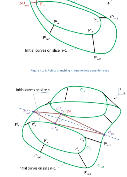
FIGURE 4.1-3.LOFTING PROCEDURE FOR 3 SLICES (SEE EXPLANATIONS IN TEXT) ... 74

FIGURE 4.1-4.POINTS BRANCHING IN ONE-TO-ONE TRANSITION CASE ... 77

FIGURE 4.1-5.TWO-IN-ONE TRANSITION CASE ... 77

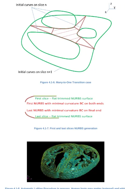
FIGURE 4.1-6.MANY-TO-ONE TRANSITION CASE ... 78

FIGURE 4.1-7.FIRST AND LAST SLICES NURBS GENERATION ... 78

FIGURE 4.1-8.AUTOMATIC LOFTING PROCEDURE IN PROCESS.HUMAN BRAIN GREY MATTER (EXTERNAL) AND WHITE MATTER (INTERNAL)NURBS FOR 7 MID-BRAIN SLICES ... 78

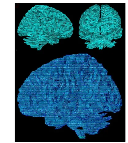
FIGURE 4.1-9.WHITE MATTER EXTERNAL NURBS SURFACES AFTER LOFTING PROCEDURE IMPLEMENTATION ... 80

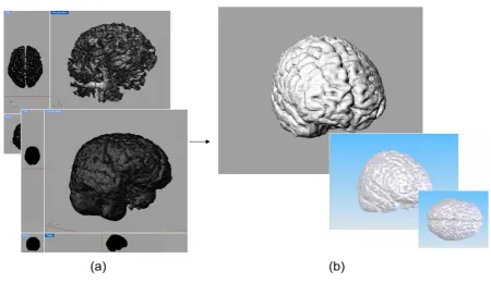
FIGURE 4.1-10.(A)POLYGONAL SMOOTHING OF THE WHITE AND GREY MATTER.(B)SOLID CAD MODEL REPRESENTATION ... 81

FIGURE 4.1-11.FINAL CAD WHOLE-BRAIN MODEL.WHITE MATTER OUTLINE ... 82

FIGURE 4.1-12.FINAL CAD WHOLE-BRAIN MODEL.GREY MATTER OUTLINE ... 83

FIGURE 4.2-1.THE POSITION OF THE DETECTION SURFACE IN RELATION TO THE BRAIN MODE ... 85

FIGURE 4.2-2.THE FE MODEL AND MESH SAMPLE ... 85

FIGURE 4.2-3.MESH CONVERGENCE GRAPH ... 86

FIGURE 4.2-4.MAGNETIC FIELD PRODUCED BY THE VERTICAL STRAIGHT CURRENT SOURCE MAPPED ON THE DETECTION SURFACE .... 87

FIGURE 4.2-5.THE RESULTING MAGNETIC FIELD PRODUCED BY THE VERTICAL STRAIGHT CURRENT SOURCE MAPPED ON THE CENTRAL SLICE (WHITE MATTER) FOR THE OPTIMAL MESH SIZE ... 87

FIGURE 4.3-1.ANISOTROPIC CONDUCTIVITY DISTRIBUTION.COLOR PALETTE SHOWS THE MAIN AXIS OF ANISOTROPY. ... 92

FIGURE 4.3-2.THE LEVEL OF ANISOTROPY IN THE BRAIN.FROM GREEN (ISOTROPIC) TO RED (HIGHLY ANISOTROPIC) ... 93

FIGURE 4.3-3.EXAMPLE OF THE ANISOTROPIC CONDUCTIVITY TENSOR DATA FOR EACH ELEMENT OF THE SPACE. ... 94

FIGURE 4.3-4.THREE SLICES OF THE COARSE FE MODEL WITH THE CONDUCTIVITY PROPERTIES OF EACH ELEMENT ... 95

FIGURE 4.4-1.FORMULATION OF THE TEST PROBLEM ... 97

FIGURE 4.4-2.RESULTS OF TEST SIMULATION: GLOBAL CURRENT DENSITY VECTOR PLOTS ... 99

FIGURE 4.4-3.RESULTS OF TEST SIMULATION: VISUALIZATION OF THE CURRENT PATH INSIDE THE BRAIN STRUCTURE ... 100

FIGURE 4.4-4.RESULTS OF TEST SIMULATIONS: CURRENT PATH TOPOGRAPHIC VIEWS.COLOR LEGENT REPRESENTS CURRENT DENSITY MAGNITUDE VALUE.NOTICE NONLINEARITY OF THE PATH DUE TO ANISOTROPY ... 101

FIGURE 4.4-5.CURRENT PATH RECONSTRUCTION ALGORITHM (SEE TEXT FOR EXPLANATIONS). ... 105

FIGURE 4.4-6.CURRENT SOURCE IN THE TEST CASE PROBLEM ... 106

FIGURE 4.4-7.POSITION OF THE CURRENT SOURCE IN TEST ANALYSIS (RED RECTANGLE) ... 107

FIGURE 4.4-8.CURRENT DENSITY DIAGRAMS FOR DIFFERENT CONDUCTIVITY VALUES ... 110

FIGURE 4.4-9.DIRECT SUBMODELLING ROUTINE DESCRIPTION IN APPLICATION TO SINGLE BEAM CONDUCTANCE PROBLEM ... 112

(11)

List of Figures

_____________________________________________________________

FIGURE 4.4-11.MESH CONVERGENCE GRAPH COMPUTED FOR MAGNETIC FIELD FLUX DENSITY VALUE CALCULATED AT THE CRITICAL

POINT OF INTEREST R=0.006M FROM THE CENTER OF THE CONDUCTOR ... 116

FIGURE 4.4-12.MAGNETIC FIELD DENSITY DIAGRAM FOR CASE WITH CONDUCTIVITY OF 10S/M AND OPTIMAL MESH... 116

FIGURE 4.4-13.OPTIMAL NUMBER OF MATERIAL PROPERTIES IN THE MODEL P AS A FUNCTION OF TOTAL NUMBER OF FE ELEMENTS N ... 117

FIGURE 4.5-1.OUTLINE OF THE OPTIMAL FINITE ELEMENT MODEL MESH FOR GREY (TOP) AND WHITE (BOTTOM) MATTER RESPECTIVELY ... 120

FIGURE 5.1-1.ACTION POTENTIAL PROPAGATION AND CURRENT DISTRIBUTION ... 122

FIGURE 5.1-2.CURRENT DISTRIBUTION PROPAGATION IN TIME ... 122

FIGURE 5.1-3.CABLE THEORY'S SIMPLIFIED VIEW OF A NEURONAL FIBER; RM– MEMBRANE RESISTANCE, RL– LONGITUDINAL RESISTANCE, CM– CAPACITANCE DUE TO ELECTROSTATIC FORCES ... 123

FIGURE 5.1-4.EQUIVALENT PROBLEM FORMULATION FOR MAGNETIC ANALYSIS ... 124

FIGURE 5.1-5.COMPUTATIONAL SCHEME FOR FORWARD PROBLEM MAGNETIC ANALYSIS;VC IS THE VELOCITY OF ACTION POTENTIAL PROPAGATION (10 M/SEC) ... 125

FIGURE 5.2-1.FLOATING COORDINATE SYSTEM FOR MATHEMATICAL COMPUTATIONS ... 127

FIGURE 5.2-2.MATHEMATICAL PARAMETERS OF THE ACTION POTENTIAL APPROXIMATION ... 129

FIGURE 5.3-1.MULTIPLE THIN FIBER FORMULATION ... 134

FIGURE 5.3-2.MYELINATED FIBERTRACT FORMULATION ... 134

FIGURE 5.3-3.NEURONAL CLUSTER FORMULATION ... 135

FIGURE 5.4-1.NOVEL INVERSE PROBLEM APPROACH.WHITE MATTER FIBERTRACTS ACTIVATION DETECTION, WHICH LEADS TO THE ACTIVATED CORTEX ZONES MAPPING. ... 137

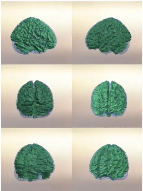
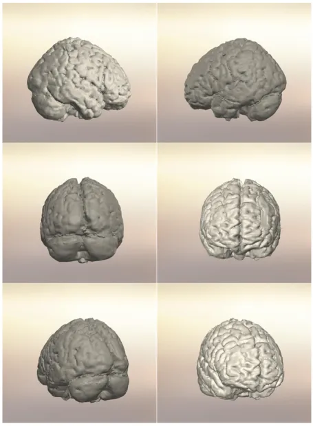
FIGURE 5.4-2.WHITE MATTER FIBERTRACTS RECONSTRUCTION .TOP ROW SHOWS WHOLE-BRAIN FIBERS, MIDDLE ROW SHOWS FIBERS LONGER THAN 18MM, AND BOTTOM ROW SHOWS FIBERS LONGER THAN 30MM.COLUMNS REPRESENTS FROM LEFT TO RIGHT:RIGHT,SAGITTAL, AND ANTERIOR VIEW RESPECTIVELY ... 140

FIGURE 6.1-1.VOLTAGE LOAD, OBTAINED FROM SPM DATASET FOR EACH OF THE CURRENT SOURCE AND ASSUMED DISTRIBUTION (BLACK POINTS ON THE IMAGES MATCHES THE MODELED SOURCES IN FEM) ... 150

FIGURE 6.1-2.CURRENT SOURCE MODELING APPROXIMATION ... 150

FIGURE 6.1-3.POSITION OF THE CURRENT SOURCES ‘1’,’2’, AND ‘3’ IN FE MODEL ... 151

FIGURE 6.1-4.POSITION AND FORM OF THE DETECTION SURFACE (BOTTOM LEFT - ACTUAL POSITIONS OF THE SQUID SENSORS) .. 152

FIGURE 6.2-1.RESULTS.MAGNETIC FIELD FLUX DENSITY VECTOR DISTRIBUTION ON THE DETECTION SURFACE ... 153

FIGURE 6.2-2.RESULTS.CURRENT DENSITY VECTOR PLOT INSIDE THE BRAIN STRUCTURE ... 154

FIGURE 6.2-3.RESULT.CURRENT DENSITY INTENSIVE PLOT ... 155

FIGURE 6.2-4.COMPARISON OF THE FEM RESULT (LEFT) AND REAL EXPERIMENTAL RESULT (RIGHT).MAGNETIC FIELD FLUX DENSITY PLOT ON THE DETECTION SURFACE.TIME FRAME -200MS. ... 156

(12)

List of Figures

_____________________________________________________________

FIGURE 7.2-1.ELECTRIC CURRENT DENSITY VISUALIZATION.FROM INITIAL TIME 0MS (TOP LEFT) TO THE FINAL TIME 10MS (BOTTOM RIGHT) RESPECTIVELY ... 164

FIGURE 7.2-2.CURRENT DENSITY VECTOR DISTRIBUTION.TIME POINT T=5MS.VECTOR SIZES DEPEND ON MAGNITUDE ... 165 FIGURE 7.2-3.CURRENT DENSITY VECTOR DISTRIBUTION.CLOSER LOOK AT AN ARBITRARY CHOSEN TIME FRAME T=1.5MS.CONSTANT VECTOR SIZES... 165 FIGURE 7.2-4.POSITION OF THE OBSERVED POINTS FOR MAGNETIC FIELD MEASUREMENTS ON THE MEG DETECTORS SURFACE .... 166 FIGURE 7.2-5.MAGNETIC FIELD FLUX DENSITY FOR EACH CORRESPONDING DETECTING POINT ... 166 FIGURE 7.4-1.OUTLINE OF THE BRAIN MODEL AND POSITION FOR THE SUBMODELLING REGION AND NEURONAL SOURCE... 170 FIGURE 7.4-2. RESULTS OF SIMULATIONS.COMPARISON BETWEEN THE INITIAL COARSE MODEL SOLUTION (LEFT), FINE MODEL

SOLUTION (MIDDLE), AND CSR SOLUTION (RIGHT).ROWS REPRESENT TOP AND SIDE VIEWS RESPECTIVELY ... 172 FIGURE 7.4-3.CURRENT DENSITY DISTRIBUTION INSIDE THE SUBMODELLING REGION OF THE COARSE MODEL.DIRECT COARSE MODEL

SOLUTION (LEFT), AND SOLUTION AFTER CSR(RIGHT) ... 173 FIGURE 7.4-4.MAGNETIC FLUX DENSITY ISOSURFACE PLOT FOR COARSE MODEL (LEFT) AND WITH SUBMODELLING APPROACH (RIGHT)

... 174

FIGURE 7.5-1.COMPARISON BETWEEN ANALYTICAL AND SIMULATED CURVE OF DEPENDENCE BETWEEN THE MAXIMAL MAGNETIC FIELD IN THE SENSOR AND FIBERTRACT DIAMETER ... 177 FIGURE 7.5-2.MAGNETIC FIELD FLUX DENSITY NORMAL TO THE SENSOR SURFACE PLOT IN CASE OF REALISTIC FIBERTRACT DIAMETER

(13)

List of Tables

_____________________________________________________________

List of Tables

TABLE 2-1.COMPARISON OF THE DIFFERENT METHODS WITH RESPECT TO MODELING ... 49

TABLE 4-1.PARAMETERS OF THE SOLID NURBS MODEL OF THE HUMAN BRAIN ... 79

TABLE 4-2.PARAMETERS OF THE FE MODEL ... 84

TABLE 4-3.PARAMETERS OF THE MODEL WITH ANISOTROPIC PROPERTIES... 98

TABLE 4-4.TOTAL CURRENT VALUES AND AVERAGE DEVIATION IN DIFFERENT CASES ... 110

TABLE 4-5.FINAL OPTIMAL PARAMETERS OF THE BRAIN MODEL ... 119

TABLE 7-1.PARAMETERS OF THE SIMULATIONS FOR NEUROTRACT (FIBERTRACT) ACTIVATION ... 162

TABLE 7-2.ABSOLUTE DISTANCES FROM THE MEASURING POINT TO THE PATH ... 167

(14)

Introduction

_____________________________________________________________

Chapter 1 Introduction

1.1 Preface

The term magnetic-field tomography (MFT) refers to a relatively new imaging modality which involves localization and subsequent imaging of active areas in the brain by measuring the extremely weak neuromagnetic fields (10–100 fT) produced by neural currents in these areas associated with cognitive processing (magnetoencephalogram). This approach, called the magnetoencephalography (MEG) technique (recording of magnetic fields produced by electrical activity in the brain), is the only truly non-invasive method which could provide information about functional brain activity.

The MFT, based on MEG data, would provide images of the brain “at work” and, as such, could have major implications for neurology and neuropsychiatry, in general, and new instrumentation for diagnosis in particular. Compared to other imaging modalities [e.g., computed tomography (CT), positron emission tomography (PET), single photon emission computed tomography (SPECT), magnetic resonance imaging (MRI)], the MEG technique is the only imaging modality that combines high temporal with high spatial resolution.

Due to its advanced properties, MEG can be used in the wide range of clinical applications which requires very precise knowledge about working human brain. It was shown to have enormous potential to be used in the study of stroke, autism, schizophrenia, Alzheimer's disease, Parkinson's disease, and cognitive and mental disorders.

(15)

Introduction

_____________________________________________________________ known generators (sources) in the brain and 2) the inverse problem of localizing and imaging the generators by using MEG data measured around the head, and the data obtained from the forward solution. Besides, an accurate solution of the forward problem has implications for design, configuration, and placement of superconducting quantum interference device (SQUID) sensors, used to measure the neuromagnetic fields around the head, and which constitute the sensing subsystem of the MFT system. Thus, the successful solution of the inverse problem and, hence, the effectiveness of the MFT as a whole is very much dependent upon the accurate solution of the forward problem.

Despite the growing interest of MEG application in clinical studies, the main research activity is focusing on inverse problem solution in order to accelerate the beginning of successful clinical implementation. However, recent studies highlighted the growing gap between the accuracy of forward problem solution and inverse solution methods. None of the existing methodologies can satisfy the accuracy requirements which are dictated by the theoretical assumptions underlying already existing methods of the inverse problem solution.

At the same time new hardware and components were introduced by various MEG equipment manufacturers. A number of these components allow improving the accuracy of acquiring data and measurements of the magnetic fields around the human head, and reducing background noise. All together in combination with the improving signal processing methodologies it also illuminates the need of improvement for the methodologies of the forward problem solution.

This work presents the complete set of methodologies for accurate solution of the forward problem via incorporating realistic brain geometry and inhomogeneous anisotropic material properties coupled with the new realistic neuronal current source approximations.

(16)

Introduction

(17)

Introduction

_____________________________________________________________

1.2 Aims and Objectives

Based on the existing research problems discovered during the literature survey (see Chapter 2) and on-going research activity observation the following aims can be formulated:

Aim 1: Improve the methodologies for the human brain modelling for forward solution MFT based on MEG. This aim refers to the following objectives:

1) Develop and test the realistic brain model according to fundamental physiological, biological and geometrical basis

2) Create algorithms and procedures for automatic brain model reconstruction with required optimization of parameters and accuracy. Developed methodologies must be patient (subject) specific

Aim 2: Develop methodologies for neuronal current source modelling for forward and inverse problem in MFT based on MEG. Objectives related to this aim are:

1) Create realistic neuronal source model for MEG forward problem calculations based on the bio-electro-physical underlying assumptions

2) Develop algorithms and procedures for implementation of the neuronal current source model into the human brain model for the full branch of possible problems related to the forward problem solution

3) Prove that developed neuronal source model can be used for inverse problem solution

Aim 3: Approximate possible errors of developed methodologies and experimentally validate them. Specified aim leads to the following list of objectives:

1) Obtain optimal modelling and solution parameters for required accuracy

2) Achieve the required computational accuracy using developed model for the simple testing solution

(18)

Introduction

(19)

Literature Survey

_____________________________________________________________

Chapter 2 Literature Survey

2.1 History of Magnetoencephalography (MEG)

The history of non-invasive medical neuroimaging began with the radiographic technique introduction by Professor Wilhelm Conrad Roentgen [1]. It was a great step towards understanding of how human brain works and at that time the only non-invasive method of clinical studies and monitoring. The idea of radiographic technique is based on the evaluation of internal body images using the X-ray. This technique could provide these pictures for internal human body and therefore the brain because of difference in absorption of X-ray in different tissues. Unfortunately human brain is almost entirely composed of soft tissues that are not radio-opaque, and it is almost impossible to see the structure of the tissues inside the brain for adult people. This is also true for the most brain abnormalities, especially those ones which do not affect density changes. At the same time radiographic technique is very dangerous due to high level of radiation dose which patient receives when doing X-ray scan.

(20)

Chapter 2

Literature Survey

_____________________________________________________________ Modern noninvasive medical neuroimaging started with the development of cerebral angiography [2]. This method is based on injection of the radioactive contrast into the blood system, and then detection of the traces produced by this contrast. This technique is used nowadays with slight modification of processes and allows very accurate imaging of blood vessels in the entire human brain.

Computerized Tomography (CT) and Magnetic Resonance Imaging (MRI), together with functional MRI, Positron-Emission Tomography (PET), and Single Photon Emission Computed Tomography (SPECT) are the main established methods which nowadays are used to provide noninvasive brain scanning, but all of them have their limitations, practical and theoretical. CT does not provide enough accuracy and it is relatively destructive. MRI has low spatial resolution, which cannot be improved theoretically due to fundamental limitations. PET and SPECT are extremely destructive because of the radioactive contrast.

There is also a technique have been developed in the field of combining these procedures [3] in order to get more accurate images and make described modalities less dangerous. The combination of several methods implemented together to work simultaneously is called Multimodal Neuroimaging.

(21)

Literature Survey

_____________________________________________________________ electrode signal however consists of not only the electrical signal of neuronal activity, but also contains entire intercellular eddy currents and external noise.

The limitations of EEG have been successfully passed with the development of Magnetoencephalography (MEG) method and the Magnetic-Field Tomography (MFT) related to it. As mentioned earlier in Chapter 1, MEG deals with measuring the neuromagnetic fields produced by neural currents in these areas associated with cognitive processing.

First magnetoencephalogram was measured by University of Illinois physicist David Cohen in 1968 [4] using only a copper induction coil as the magnetic field detector. The measurements were made in a magnetically shielded room in order to reduce the magnetic background noise. However, the insensitivity of this detector resulted in poor, noisy MEG signals, which were difficult to use. Then later he built a better shielded room, and used one of the first Superconductive Quantum Interference Devices (SQUID), just developed by James E. Zimmerman, a researcher at Ford Motor Company [5] to measure the MEG again [4]. This time the signals were almost as clear as an EEG. Obtained results stimulated the interest of physicists who had begun looking for uses of SQUIDs.

Nowadays MEG is the most promising technique (it is currently on the experimental stage) because it is the only imaging modality that combines high temporal with high spatial resolution. As mentioned before, it is relatively young and not fully developed yet mainly due to lack of understanding of electromagnetic processes involved in cognitive activity.

(22)

Chapter 2

Literature Survey

_____________________________________________________________

2.2 Principles of MEG

Human brain consists of the assembly of neurons, which generate electrical activity (electrical impulses) and exchange this activity with each other [6]. The structure of the single neuron is shown in Figure 2.2-1. Single neuron consists of a cell body which is the central part, axons, dendrites, and synaptic terminals. Neuronal axon is the main electrical signal provider. Dendrites are the signal receivers, and synaptic transmitters are playing electrochemical neuron-to-neuron signal exchange role. Neurons are generally combined into the formations. Clustered formations of the neurons in cerebral cortex are also known as neuroclusters. All together they form neo-cortex, which is so-called grey matter. Grey matter is the thin (2-3mm [7]) layer which covers the brain volume and thought to be the part of the brain responsible for cognitive activity. The internal part of the brain is called white matter. White matter mostly consists of neuronal chains called neurotracts or fibertracts as they form a fiber structure. There are two types of fibertracts depending on the surrounding cells: myelinated and unmyelinated. Myelinated tracts consist of neurons which are surrounded by myelin shield. Myelin acts as ion source protector and at the same time provides mineral‟s supply to the neuron. Unmyelinated fibertracts are mostly located in very packed areas of the nervous system (such as areas which are close to cerebral cortex or cerebellum).

(23)

Literature Survey

_____________________________________________________________ Due to the intracellular and extracellular electrochemical activity of neuronal cell and mechanisms of electric impulses propagation neurons act as magnetic and electric fields generators. Magnetic field produced by neuronal activity can be measured and associated to bio-chemical activity. Collected data could provide essential information about initial electrical activity, such as position of activated neurons and internal current paths between different brain zones.

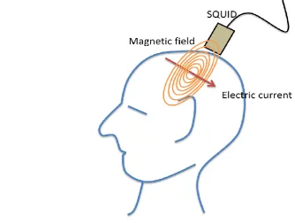
As described before, MEG use the SQUID sensors positioned around the human head in order to perform required measurements. Obtained information then is meant to be processed and interpreted by medics according to physiological and personal structures for particular subject. Basic MEG-based magnetic field tomography scheme is demonstrated in Figure 2.2-2.

[image:23.595.72.407.481.733.2]

(24)

Chapter 2

Literature Survey

_____________________________________________________________

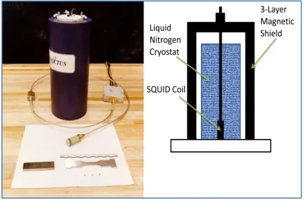
[image:24.595.72.513.95.384.2]

The magnetic superconductive coil itself is not simple and is based on state-of-the-art technology which involves inclusion of complex superconductive wires in optimally-shaped superconductive metal loop. Example of modern coil could be seen in Figure 2.2-4 [9]. Generally MEG measurements involve information processing from several sensors placed around the head of the analyzed subject. It is now convenient to use about 140-300 sensors [10] in order to get acceptable accuracy for the following signal processing procedure. However the number of electrodes and its placements are still open questions for researchers. One of the relatively new MEG machine can be seen in Figure 2.2-5. The illustrative layout of SQUID sensors within this particular machine can be found in Figure 2.2-6 [11].

(25)

Literature Survey

_____________________________________________________________

[image:25.595.65.476.90.761.2]

(26)

Chapter 2

Literature Survey

_____________________________________________________________

(27)

Literature Survey

_____________________________________________________________

2.3 Basics of the Forward Problem

Like every other tomography technique, MEG involves solution of two different problems, which are both important for understanding of the relations between measured data and actual physical processes, actual hardware manufacturing, data processing, results interpretation, and clinical applications. The idea of forward and inverse problems specification is illustrated in Figure 2.3-1.

(28)

Chapter 2

Literature Survey

_____________________________________________________________ obtaining magnetic fields around the head as much close to reality as possible. Basically, forward problem in case of MEG includes simulation of whole electromagnetic processes within the head and validation of the results with the experimental data. This simulation requires performing of all range of engineering routines, from the very abstract mathematical problem formulation to the complex numerical analysis, optimization, accuracy estimation etc.

In order to create a good basis for inverse problem solution it is important do discover all possible ways of mathematical simulation and to obtain the best possible way of modelling for such complex process. Successful forward problem solution allows optimization in terms of accuracy, time of computation, practical realization and cost-effectiveness of the required methodologies and apparatus [12]. There are many different ways of doing so (as shown in next Section) and one of the main proposes of this study is to choose or create the more reliable one from the very beginning.

(29)

Literature Survey

_____________________________________________________________

Forward model is ready for investigation after all computational requirements are achieved. Initial study usually involves realistic simulation tests. This is essential in order to get methodology restrictions and computational restrictions. Also forward modelling tests are required for understanding fundamental theory of processes, which take place within human brain. A part of investigation activity is concentrated in the field of exploring the mechanisms of different diseases such as epilepsy, Parkinson‟s disease, etc. Huge research interest is also associated with the mechanisms of the human thinking process as it is still unknown. It is also very important to have a right computational model with the ability of simulations to be performed for the different neuronal sources activation approaches. Thus for all of research activity which is based on the forward problem it is essential to be sure that forward model has good predictability and accuracy.

(30)

Chapter 2

Literature Survey

_____________________________________________________________ As mentioned before the significant part of research activity which is based on forward modelling is focused on the brain matter disorders. Forward model must predict the electromagnetic processes which take place inside the degraded human brain (without one or many functional parts). The most known case of such brain matter disorder is Alzheimer disease. The brain of the subject affected with disease has strongly degenerative matter. There is a huge interest in understanding the way that signals are processed inside neuronal structure of the brain degraded by this disease. Successful forward problem solution in combination with the latest imaging technologies could help create the fundamental structure for further experimental investigations.

Forward problem in application to MEG tomography consists of three fundamental concepts (first three boxes in Figure 2.3-2), that has to be defined before starting any simulations and investigations. First of all it is the type of the brain model, which would be considered in the analysis in form of modeled physical object. It can have geometrical representation (spherical, realistic-shaped, etc.), or some abstract mathematical interpretation and should satisfy the forward problem conditions. Second concept is the type of neuronal current source which is used as an electrical source for forward model (existing approaches to current source modelling is shown in next chapter). Finally, it is essential to choose computational method for solving the appropriate system of mathematical equations followed from the mathematical model.

The mathematical structure of the forward MEG problem is fully determined by the physical Maxwell equations, discussed in Chapter 3, therefore the first box in Figure 2.3-2 for MEG involves only simplification of mathematical model and investigation of the solution method. The requirements for the human brain model and neuronal source model (such as geometrical and material accuracy) are much stronger than solution method parameters (such as time of computation or cost-effectiveness). Hence in case of MEG the brain model and source are determined first and then the right solution method is revised.

(31)

Literature Survey

(32)

Chapter 2

Literature Survey

_____________________________________________________________

2.4 Literature Survey

2.4.1 Models of the Human Brain

The importance of accurate human brain reconstruction is followed from the Maxwell equations and it is one of the most discussed topics inside the scientific society related to the tomography problems. Great influence of even small particular disturbance of the input data on the final solution is specifically mentioned in wide range of papers [13-18]. However, all possible brain models will be revised in this paragraph in order to show the historical developing and possible basic engineering solutions for solving this problem.

2.4.1.1 Spherical and Ellipsoidal Models

Early stages of research related to MEG tomography forward problem were quite basic due to the lack of the computational resources. The aim of forward modelling at that time was to understand the possible ways of obtaining the solution on primitive level. Most of the methods which were used during the studies are formulated in general with the simple example which is placed in order to illustrate the method and to get engineering approximation of the solution.

The spherical brain model was considered as a good computational approximation at the very beginning of the MFT development. Spherical models in papers [19-27] showed the limitations of MEG technique in general and were used to obtain the preliminary range of possible ways to improve the computational technique and the solution method. However, the results obtained with spherical models were very inaccurate, and it was shown [17, 18, 20, 28-32] that they cannot be used to calculate magnetic fields around the head in any case of practical application.

(33)

Literature Survey

_____________________________________________________________

resulting magnetic fields were obtained and the direction of improvement work has been set up. The solutions of the problem, as stated before, were far beyond the limits of accuracy [22].

The layered spherical brain model has been developed as an improvement to the single solid sphere. Each single layer of the model represents different tissues of the physical human head. There could be different number of layers, but the most common is 3 layer schemes with scull bone, white and grey matter subdivision (Figure 2.4-1).

The layered spherical model shows almost the same poor accuracy of the solution as a homogeneous one and it was shown [22] that the main influence on the accuracy is the geometrical shape of the head, which is far away from spherical in reality. The first attempt of the shape improvement was made by assuming the head to be an ellipsoid [29, 34, 35]. This was quite reasonable engineering improvement considering the fact that elliptical model still allows analytical computation of the magnetic field around the head. Also ellipsoidal model gave quite a few improvements to the final forward problem solution. However the resulting magnetic field distributions were found not matching any reasonable limit of accuracy. The

(34)

Chapter 2

Literature Survey

_____________________________________________________________ and white matter of the brain are much more complex in terms of geometry than any smooth-surfaced structure. In order to understand this complexity and difference with the ellipsoid let us consider the following example.

Imagine the flat A4-formatted piece of paper. If wrinkled (see Figure 2.4-2) this object can visually represent the brain surface layout with approximately the same geometrical level of complexity. The external shape of wrinkled sheet can be approximated by ellipsoid. The area of approximating elliptical body will be more than 6 times less than the initial area of A4. Thus even rough estimation shows the difference of the resulting solution to be more than 6 times. In reality the difference can be more than 20 times (mostly due to the hidden high-packed surface areas such as cerebellum). So even if one needs to calculate the simple area of the surface for grey matter, in reality this is much bigger than in case of spherical or ellipsoidal shape.

Studies show that all sufficient matter transition regions are very important during the simulations [30]. Therefore the realistic shape of the model is strongly required for forward problem solution. The improvement and sufficient increase of the accuracy due to realistic shape modelling is observed in next paragraph.

(35)

Literature Survey

_____________________________________________________________

2.4.1.2 Realistically Shaped Brain Models

Increased computational resources and computer evolution allow solving the problem in constructing realistically shaped brain models. In paper [20] the influence of the human brain shape was first introduced and studied. The strong difference between spherical and realistically shaped models for MEG forward simulations was shown. Also the importance of complexity of the brain external structure was discovered. The model itself is illustrated in Figure 2.4-3. Despite the fact that even this shape is far beyond the realistic, the difference between this and elliptical model was sufficient enough to propose realistic brain model as gold standard for such simulations. Further investigations showed even more the importance of the brain geometrical shape being accurately modeled. In work [18] the internal structure of the brain tissues was found as one of the main influence on the accuracy of the solution. The main advantage of the work was in the comparison of the simulating results with experimental data. The magnetic field mapping indicated similarity of the magnetic field outline to the maps obtained from experiment. However the numerical values were found not matching experimental ones.

(36)

Chapter 2

Literature Survey

_____________________________________________________________ geometry of the grey matter. At the same time different material properties have been applied to the parts of the model corresponding to grey, white matter and cerebrospinal fluid (CSF). In Figure 2.4-4 an example of such model is shown [32]. The work mainly concentrated on EEG forward simulations. For EEG analysis the muscle and scull tissues are important due to current redistribution, therefore the main part of the model consists of mainly these tissues with the lack of geometrical detailing within the brain itself. For MEG forward simulations it is unnecessary to consider muscle, scull and CSF due to high conductivity contrast between brain matter and other surrounding tissues.

In works [16, 17] the importance of the material properties being considered properly is also confirmed. The simple division on grey and white matter, which is considered in majority of previous work, is found to be not enough in order to satisfy the requirements of the forward problem solution. Further investigations with the new imaging modality called Diffusion Tensor Magnetic Resonance Imaging (DTMRI) proposed new method for material properties extraction on the very high level of accuracy. This method highlighted very high anisotropy of the material properties, particularly electrical conductivity, within the brain white matter. The only attempt to

(37)

Literature Survey

_____________________________________________________________ apply such complex conductivity properties was made in paper [32]. The overview of the brain model with anisotropic properties which has been used in this study is shown in Figure 2.4-5.

High influence of the conductivity tensor anisotropy on forward problem solution results was highlighted. However in this paper a relatively complicated algorithm was introduced and unusual software package was developed in order to allow such computations. Due to the methodology that was chosen to introduce these computations it is very difficult to use models developed in [32] for the following research. Particularly, this algorithm does not allow applying realistic current sources. Due to internal format which is used for anisotropy classification and storage of analyzing data it is very difficult to convert and transfer the modeled geometry and material properties to other formats and computational packages. In recent years several papers were published where attempts of combination with using different types of models and realistic material properties were made in application to MEG research and particularly forward problem solution. For example, elliptical brain model was combined with realistic material properties in [34]. Also some improvements were made to geometrical modelling of the human brain in [37, 38]. In this entire branch of works the importance of accurate geometrical in combination with accurate material properties modelling is proved. However there is a big gap in terms of practical application for those mathematical methods and integration of models into the forward solution.

(38)

Chapter 2

Literature Survey

_____________________________________________________________

Figure 2.4-5. Coregistered T1-weighted magnetic resonance image (a) and diffusion tensor (b), FEM model cross section (c), and setup for the simulations (d). The white square in (a) indicates the region of

interest enlarged in (b). The diffusion tensor image was interpolated to match the spatial resolution of the T1 image. The ellipsoids depict the local diffusion tensor. The ellipsoid axes are oriented in the

(39)

Literature Survey

_____________________________________________________________

2.4.2 Models of the Neuronal Current Source

Neuronal current source which is applied in forward problem traditionally is described considering biological formations as a single neuron, neuronal chain, or neuronal cluster (assemble of neurons). Neuronal chains also can create assemblies known as neurotracts, or fibertracts. Entire white matter mostly consists of neurotracts, although grey matter in general is the assembly of neuronal clusters [39]. The neurons of the grey matter (cerebral cortex) are known as main functional cells of the brain responsible for cognitive activity, and therefore in almost all MEG research papers only this type of neurons is considered (Figure 2.4-6). Typical cortical neuronal distribution in grey matter is shown in Figure 2.4-7.

(40)

Chapter 2

Literature Survey

_____________________________________________________________

(41)

Literature Survey

_____________________________________________________________

(42)

Chapter 2

Literature Survey

_____________________________________________________________

2.4.2.1 Single Dipole Model

In the MEG and EEG research work the dipole approximation of the neuronal current source is mostly considered to be convenient to use. The basics of this approach was introduced in work [22] where the assumption of quasistatic behavior was considered and required accuracy for the linear solution and solid spherical brain model was obtained. The hypothesis of the dipole current source was given based on the fact that neuronal impulse which passes along the axon is very short in space and time; however post-synaptic electrochemical activity (the ionic current which flows between two neuronal terminals) was thought to have activation time much larger than actual axonal impulse. Therefore it could be assumed that the neuron is very short and thin current conductor that carries the current during a small period of time (between two neuronal terminals). It is very reasonable computational model for the preliminary approach because it simplifies solved equations without obvious decreasing in accuracy. In paper [23] the solution for forward problem was obtained in general form with the help of dipole model approximation. Major investigation has also been done based on the single dipole model in the field of understanding of the mechanism of current redistribution. In paper [18] the influence of the volume currents redistribution was discovered. In this work abstract conductive regions were considered, which are schematically illustrated in Figure 2.4-8, and solution was obtained in parametric form.

The importance of the volume currents was proved by calculations of the error in the dipole localization after forward and inverse problem solution. The average error without volume currents consideration (up to 62mm) was significantly larger than the error with such consideration (maximum error was 6mm).

(43)

Literature Survey

_____________________________________________________________

simultaneous activation of the neuronal current sources positioned very close to each other in common region.

At the same time distributed dipole model was offered as the possible substitution to the current source approximation for the forward problem solution.

2.4.2.2 Distributed Dipole Model

[image:43.595.68.526.90.400.2]

Distributed dipole model in general is simultaneous combination of number of single dipole models. There are several approaches to modelling and implementation of this kind of neuronal current source into the forward problem. First approach is based on the random initial distribution of the dipoles, and their activation according to the position in known specific cortical areas [40]. Second approach is based on the assumption of uniform distribution and the contrary random activation of the

Figure 2.4-8. Schematic diagram showing the relationship between r’ (coordinate of the dipole), Q (moment of dipole), r (coordinate of the detector), n„(normal to the detector), G (total conductive region), G1„(conductive

(44)

Chapter 2

Literature Survey

_____________________________________________________________ solutions, uses the specific configuration of the small group of dipoles in the activation area.

The influence of the different dipoles concentration and position, number of dipoles and orientation has been discovered in literature with the help of distributed dipole models. Sufficient sensitivity of the solution from fluctuation of all mentioned parameters was found in [20, 23, 41-43]. Below is the simple example which illustrates importance of the spatial distribution of the dipoles. Consider two dipoles which have the same magnitude but opposite direction. Imagine these dipoles being placed as close to each other as possible. Simultaneous activation of these dipoles produces zero magnetic field. The same result will take place with two pairs of dipoles, positioned anywhere in the conductive region. So it is obvious that the solution does depend on the internal parameters of the solution method, which are not the parameters of the real object (neuronal current source). There are several ways of limiting the number of parameters and therefore organizing somehow the dipole approximation [20], but all of them lead to unrealistic results by default and does not construct predictable and reliable working model.

2.4.2.3 Distributed Surface and Volume Current Models

Distributed Surface and volume sources have also been used widely in literature [44, 45]. The idea is based on using current density vector distribution inside the given conductive volume representing neuronal current source (see Figure 2.4-9). This method brought new forward simulation algorithms and precise computational results [46]. The main advantage of this approach is in applicability which is absolutely free from any limitations on type and spatial position of the current source. Also forward computations can be performed easily with using almost any solution method. The accuracy of this model in combination with realistic brain model is acceptable in comparison to any other current source approximations.

(45)

Literature Survey

_____________________________________________________________

of the same reason the solution complexity increases exponentially with consideration of more realistic multiple current source activation problems. The accuracy of the method also strongly depends on the source application accuracy. Therefore the final solution error (which is calculated with multiplying the average error by the number of applied parameters) cannot be delivered to be small enough for successful validation.

Due to such implementation complexity and infinite number of unknowns the inverse problem, which is constructed from the forward problem results with distributed current approach, is impossible to solve without additional solution limitations. Typically geometrical or physiological constrains [42] are used in order to apply these limitations. However, having in mind initial complexity of the brain model itself, and combining it with the additional anatomical or physiological complexity, this approach makes solution of the inverse problem to be extremely resource-intensive in terms of time and computational ability. In some cases distributed surface and volume current source model can be identical to distributed dipoles model. This appears when small spatial resolution of provided simulations is considerably low.

(46)

Chapter 2

Literature Survey

_____________________________________________________________

2.4.2.4 Other Neuronal Current Source Models

Some other less commonly used attempts of current source modelling were made in literature. The linear-source model was used in paper [26]. This model is based on the assumption that considers the neuronal axon as a small conductive straight line with the constant or quasistatic current. Some simulations with realistic brain model were performed showing the improvement of this model in comparison to the single dipole model. However, this approach is based on the unrealistic neuronal behavior and contradicts with real processes within the neuronal chain or neuronal cluster. So in case of realistic neuronal activation it is quite complicated to construct the modeled source and implement it into the human brain model to satisfy the conditions for accurate solution.

The multipolar expansions were suggested as a reasonable substitution to the traditional dipole model [47]. However the implementation complexity in combination with unrealistic assumptions put this method out of the consideration.

Several other methods were discovered in works [14, 41, 42, 46, 48]. All of them are based on the modified distributed dipoles model. The minor improvement was also shown in comparison to other methods, at the same time none of them are accurate enough for obtaining any realistic solutions for MEG forward problem.

2.4.3 Computational Methods for the Solution of Forward Problem

(47)

Literature Survey

_____________________________________________________________

2.4.3.1 Boundary Element Method (BEM)

The Boundary Element Method is the simplest for programming and interpreting the results [49]. This method was successfully used in works [19-22, 25, 26, 30, 42, 46, 50-54]. The main advantage of this approach is its speed and simplicity for programming and obtaining results, which is clearly shown in papers [21, 54]. The basic idea of the method is that the entire space could be divided onto finite number of solid regions with the uniform homogeneous material properties. Thus the boundary of each region could be extracted and then each boundary is triangulated. Each triangle acts as a boundary element, which has 3 nodes at the vertexes [20]. The distribution of the magnetic field inside the uniform homogeneous region could be easily computed knowing the potential on the boundary of the region, so the main computational part of the method is finding this potential from initial and entire boundary conditions (including current source) and then computing the internal field by knowing algebraic relations. The boundary potential could be calculated by discrete mathematical methods and appropriate 3D geometrical triangulation of the discovered object. The comparison of the boundary element method with other methods was shown for the case of isotropic spherical brain model in paper [19]. The main properties and advantages of BEM were proved:

- Small number of triangles and thus the time of computation is sufficiently small

- Flexibility in programming

- Good accuracy in case of modelling with small number of smooth homogeneous regions

(48)

Chapter 2

Literature Survey

_____________________________________________________________

2.4.3.2 Finite Element Method (FEM)

The Finite Element Method is based on the division of the entire geometrical space onto volume 3D elements [55, 56]. The mathematical solution is basically conducted with parametrical linearization of the complex tensor equations throughout the linear or quadratic space element division and following solution approximation. Each element can be described geometrically as parallelepiped or pyramid. Therefore complex geometrical formation becomes the assembly of simple solvable structures, which makes the problem in general to be formulated in form of the linear matrix equations. This method will is accurately described below in Section 3.3.

FEM is now used in literature more frequently than other approaches simply because of its ability to solve a very wide range of physical problems. A range of computational packages and products were developed based on this method in the field of electromagnetic simulations, such as ANSYS, Nastran, VF Opera. These types of software allow flexible solution of full spectrum of electromagnetic problems, offering exceptional stability, high level of programming optimization, and flexible interface. FEM is not so easy to program in comparison to BEM due to its geometrical basis, but it allows almost unlimited abilities in solving Maxwell equations, managing pre- and post-processing data and changing the parameters of the mathematical model underlying developed algorithms.

FEM in application to forward problem solution for MEG allows fast computations and provides accurate solution for simple problems with spherical brain models as was shown in work [23]. At the same time it is possible to improve and optimize the model at any stage [53]. Paper [14] shows the ability for inhomogeneous anisotropic material properties to be applied, which is the critical advantage as was discussed previously. Due to such wide usage a number of strong algorithms and data were accumulated almost in all areas of engineering computations including cross-platform and cross-software data transferring and result converting [55-58].

(49)

Literature Survey

_____________________________________________________________ Finally, as obtained in paper [16], this is the only method with the computational volume for unrestricted number of anisotropic properties in the model, which is necessary to consider in case of white matter fibertracts anisotropy inclusion. The summary of main advantages of the finite element method can be summarized:

- Flexibility in terms of geometrical approximation - Flexibility in terms of material approximation

- Ability to discover and improve the accuracy of the solution - Ability to operate with large number of material regions

- Ability to implement complex anisotropic properties of materials

The FEM has only one disadvantage: It is a relatively slow method in comparison to others in terms of computational time. However large computational time values can be avoided by using special techniques e.g. submodelling routine, developed by authors and accurately described in paragraph 3.3.3. Also this method is very friendly to parallel programming technique with combination to large multiprocessor systems.

2.4.3.3 Other Methods

There are some other methods were used in literature to solve the forward problem. They are briefly described below.

Array response kernels method [35] showed applicable results with the very basic modelling, however does not provide the ability of using complex geometrical brain models. Thus realistic model and therefore accurate results cannot be achieved with this method.

(50)

Chapter 2

Literature Survey

_____________________________________________________________ Lead-field interpolation [29, 59] could be used in combination with BEM or FEM to speed up the calculations. Time reduction of a factor of 3 relative to unmodified FEM can be achieved. However, it does not support realistic neuronal current source modelling.

Artificial neural network method [24] could also be used in inverse problem solution. For forward problem this class of methods can operate only in combination with random dipole source modelling.

2.4.4 Main Results and Summary from Literature Survey

According to present literature, a significant interest concerning adequate forward modelling is highlighted. There are fundamental works which show a great importance of forward modelling for MFT based on MEG. At the same time there is lack of realistic simulations in terms of both brain modelling and neuronal current source modelling. Also the importance of data reproduction and patient specific automatic brain model reconstruction was shown, which is at the same time the most significant part of the inverse problem as well.

In addition we must point out the lack of adequate neuronal current source models in literature. The most widely used approach is the current dipole model. This approximation, however does not seem to be accurate enough to produce realistic

TABLE 2-1.COMPARISON OF THE DIFFERENT METHODS WITH RESPECT TO MODELING

FDM FEM FVM BEM&I FDM&I FEM&I FVM&I

Geometry - + + + - + -

(51)

Literature Survey

_____________________________________________________________ result as discovered in details above and also in 3.4.

The interesting fact must be mentioned in conclusion to the literature survey. Almost no comparison of the forward problem simulation results to the real experimental data have been met in published research papers. This absence of the experimental validation of the forward problem is caused by extreme complexity of the actual experiment. It is also due to medical and research ethics issues together with the novelty of MEG itself as a clinical imaging technique.

(52)

Chapter 3

Mathematical Modelling of Magnetic Field of the Brain

_____________________________________________________________

Chapter 3 Mathematical Modelling of Magnetic Field of

the Brain

3.1 Mathematical Formulation of the Forward

Problem in MFT Based on MEG

The mathematical model of magnetic fields produced by bioelectric current sources in the brain is based on a set of quasistatic Maxwell‟s equations which lead to appropriate Poisson‟s equation. In doing so, it is assumed that the magnetic permeability of brain matter is the same as that of free space ( ). The quasistatic nature of the field is justified by the fact that bioelectrical activities that give rise to magnetic fields are predominantly of low frequency (from below100 Hz to less than 1 kHz). This, together with the material properties of brain matter (e.g., conductivity tensor and permittivity tensor ) suggest that in calculating the electric-field intensity and magnetic flux density vectors, the time derivative terms ⁄ and ⁄ in Maxwell‟s equations can be ignored [60]. This leads to the following set of simplified Maxwell‟s equations:

(3.1-1)

(3.1-2)

(53)

Mathematical Modelling of Magnetic Field of the Brain

_____________________________________________________________ In (3.1-1), the total current density is equal to:

(3.1-4)

where is the primary “excitation” current (or impressed current if at the cellular level) produced by electromotive force (EMF) in the conducting brain tissue. The volume current is attributed to the effect of the macroscopic electric field on charge carriers [60]. It has been shown that for a realistic brain model with inhomogeneous conductivity distribution, the magnetic field from this volume current can be comparable with that from the primary current source (e.g., dipole) [18]. Thus, the total current density becomes:

(3.1-5)

where is the electric scalar potential. The previous equations lead to the following Poisson‟s equation for the quasistatic magnetic field, the solution of which constitutes the solution of the forward problem in MFT based on MEG [60]:

( )

In Ω = Ω( )

(3.1-6)

Under appropriate boundary conditions equation (3.1-6) is solved for the unknown potential distribution ( ) by the chosen computational method. The complexity of this equation stands by the form of ( ), which is generally tensor of 3-rd range and depends on ( ) . The magnetic field ( ) at a given point

in the problem domain Ω is then found by using:

( ) ( ) ∑ ∫