Polynomial cubic splines with tension properties

Contents lists available atScienceDirect

Computer Aided Geometric Design

www.elsevier.com/locate/cagd

Polynomial cubic splines with tension properties

✩

P. Costantini

a

,

∗

, P.D. Kaklis

b

, C. Manni

c

a_{Università di Siena, Dipartimento di Scienze Matematiche ed Informatiche, Pian dei Mantellini 44, 53100 Siena, Italy} b_{National Technical University of Athens, Ship-Design Laboratory, Heroon Polytechneiou 9, Zografou 157 73, Athens, Greece} c_{Università di Roma “Tor Vergata”, Dipartimento di Matematica, Via della Ricerca Scientifica, 00133 Roma, Italy}

a r t i c l e

i n f o

a b s t r a c t

Article history:

Available online 30 June 2010

Keywords: Polynomial splines Rational functions Subdivision schemes Shape preservation Tension property

In this paper we present a new class of spline functions with tension properties. These splines are composed by polynomial cubic pieces and therefore are conformal to the standard, NURBS based CAD/CAM systems.

©2010 Elsevier B.V. All rights reserved.

1. Introduction

The popularity and the wide spreading that CAD/CAM systems have nowadays is mostly based on the efficiency of their geometric/mathematic engines. It is well known that the kernel of such systems is constituted by B-splines basis functions (or by their rational counterparts in NURBS) which are used to form curves, tensor product or Boolean sum sur-faces. B-splines have several nice properties (positivity, partition of unity, compact support, recurrence relations, etc.) but are not so flexible as required in some applications. If we think, for instance, to interpolation problems, we know that in general spline functions are notshape preserving, that is are not capable of reproducing the shape (sign of discrete curva-ture and/or torsion) of the data. In the last decades several new classes of piecewise functions of different form and with different properties have been proposed, and it is not possible to mention all of them and all their applications. Never-theless, a conspicuous part of them have properties similar to standard cubic splines and can be grouped under the name of generalized cubic splines, that is piecewise functions composed bygeneralized cubic polynomials with the following char-acteristics. The generalized cubic polynomials are taken from four-dimensional spaces; the generalized cubic polynomials depend on shape parameters, tend to affine functions for their limit values and reduce to standard cubic polynomials for other specific values; generalized splines can be constructed connecting together generalized cubic polynomials. Since the shape parameters can be locally or globally adjusted to give the generalized spline a piecewise linear appearance, they are also refereed to as splines with tension properties. Among the many possible well-known examples we mention here exponential splines (Schweikert, 1966; Späth, 1969; Koch and Lyche, 1993), rational splines(Delbourgo and Gregory, 1985; Delbourgo, 1989), non-uniform degree or variable-degree splines (Kaklis and Pandelis, 1990; Kaklis and Sapidis, 1995; Costantini, 2000).

✩ _{Work supported by INdAM – Gruppo Nazionale Calcolo Scientifico.}

*

Corresponding author.

E-mail addresses:[email protected](P. Costantini),[email protected](P.D. Kaklis),[email protected](C. Manni).

Unfortunately, commercial CAD/CAM systems are very conservative, in the sense that they are constructed to support only low degree polynomial splines and NURBS. In particular, they cannot accept the above mentioned generalized splines, which are either not polynomial or polynomial with arbitrary degree. As a serious consequence, CAD/CAM systems renounce to incorporate the recent scientific acquisitions and to gain a stronger control on the shape of curves or surfaces.

The goal of the present paper is to give a first answer in this direction, describing a new set of generalized splines with tension properties which are composed by C2 _{cubic polynomial pieces and thus can be perfectly integrated in}

ev-ery CAD/CAM system. The tools adopted are strictly connected to the Hermite subdivision scheme described in Costantini and Manni (2010b) and based in turn on the more general results of Costantini and Manni (2010a). More specifically, in Costantini and Manni (2010b) it is shown that it is possible to construct a space of C2 _{generalized splines, equipped with}

tension properties, chiefly composed by cubic pieces with the exception of some special rational pieces. Here we show how to modify the rational pieces in cubic polynomial ones while maintaining all the desired properties.

This paper is divided in five sections. In the next one we recall from Costantini et al. (2005), Costantini and Manni (2006), the basic information on generalized cubic polynomials and generalized splines, adding some new material on splines with multiple knots. The third section describes the main results of the paper, that is the substitution of the rational pieces with cubic polynomials. Section 4 describes the spline space and the construction of the B-spline basis with tension properties. Section 5 is devoted to show some examples of applications (limited, for reasons of space, to curve and surface design), and to final comments and remarks.

2. Some preliminary material

In this section we collect the material necessary for the comprehension of the paper.

2.1. Generalized cubics

Given a real function f, we denote with

˙

f the derivative w.r. to the (local) variablet and with for D f the derivative w.r. to the (global) variablex. Assume, for notational simplicity,t

∈ [

0

,

1

]

and let

P

u,v

:=

1

,

t

,

u

(

t

),

v

(

t

)

,

u

,

v

∈

C2

[

0

,

1

]

,

dim

(

P

u,v

)

=

4

.

(1)

We state the following1

Definition 1.A basis

{

B0

,

B1

,

B2

,

B3

}

of

P

u,v is a Bernstein like basis if it gives a partition of unity, is totally positive2 on

[

0

,

1

]

and it satisfies

B0

(

1

)

= ˙

B0

(

1

)

= ¨

B0

(

1

)

=

0

,

B1

(

0

)

=

B1

(

1

)

= ˙

B1

(

1

)

=

0

,

B2

(

0

)

= ˙

B2

(

0

)

=

B2

(

1

)

=

0

,

B3

(

0

)

= ˙

B3

(

0

)

= ¨

B3

(

0

)

=

0

.

(2)

Assuming that

P

u,v has a Bernstein like basis, we denote by

ξ

0,

ξ

1,

ξ

2,

ξ

3the Greville abscissas, that ist

=

3q=0

ξ

qBq

(

t

).

In the following we assume

0

=

ξ

0

< ξ

1

< ξ

2

< ξ

3

=

1 (3)

and we associate to any element

ψ

of

P

u,v,

ψ(

t

)

:=

3

q=0bqBq

(

t

),

its Bézier control polygon (or simply control polygon) that is the polygonal line

with vertices (Bézier control points)

(ξ

0

,

b0

)

,

(ξ

1

,

b1

)

,

(ξ

2

,

b2

)

,

(ξ

3

,

b3

)

. The Bézier control polygon

closely imitates the shape of

ψ,

in the sense specified in Peña (1995), Chapter 3.

From the more general results of Costantini et al. (2005), Goodman and Mazure (2001), Costantini and Manni (2006), we infer the following proposition.

Proposition 1.If the functions u and v are such that

{¨

u

,

v

¨

}

is a Chebyshev System in

[

0

,

1

]

,

(4)

then

P

u,vhas a Bernstein like basis and(3)holds.

Without loss of generality, we can putu

=

B0,v

=

B3

.

If (4) holds,

P

u,v“behaves” as cubic polynomials (

P3

) and reduces to it whenu

(

t

)

:=

(

1

−

t

)

3,v

(

t

)

:=

t3_{. For this reason spaces}

_P

u,v are usually referred to asgeneralized cubics.

1 _{In this context we are dealing with functions of classC}2_{. In case spaces of less regularity are of interest, different definitions of Bernstein like bases} can be provided. ForH C1_{subdivision schemes see, e.g., Sablonnière (2004).}

2 _{A sequence of functions{φ}

0, . . . , φn}is totally positive on a given intervalIif for any pointst0<t1<· · ·<tminIthe collocation matrix(φj(ti))mi=0 n

We recall from Costantini and Manni (2010b) an alternative expression for

ψ

useful in the sequel:

ψ (

x

)

=

e0B0

(

x

)

+

r

(

x

)

+

e1B3

(

x

)

=

e0u

(

x

)

+

r

(

x

)

+

e1v

(

x

),

(5)

where

r

(

x

)

:=

b2

−

b1

ξ

2

−

ξ

1

(

x

−

ξ

1

)

+

b1

,

e0

:=

b0

−

r

(

0

),

e1

:=

b3

−

r

(

1

)

and the following properties

ψ (ξ

0

)

=

b0

,

ψ(ξ

˙

0

)

=

(

b1

−

b0

)

(ξ

1

−

ξ

0

)

,

ψ (ξ

¨

0

)

=

e0u

¨

(

0

),

ψ (ξ

3

)

=

b3

,

ψ(ξ

˙

3

)

=

(

b3

−

b2

)

(ξ

3

−

ξ

2

)

,

ψ (ξ

¨

3

)

=

e1v

¨

(

1

).

(6)

In many practical applications, for the definition of (1) functions of the form

u

=

u

(

t

;

α

),

v

=

v

(

t

;

β)

are used, where

α

, β

aretension parameters,3 that is are such that

u

(

t

;

3

)

=

(

1

−

t

)

3

,

v

(

t

;

3

)

=

t3

,

lim

α→+∞u

(

t

)

=

α→+∞lim u

˙

(

t

)

=

α→+∞lim u

¨

(

t

)

=

0

,

t

∈ [

a

,

1

]

,

a

>

0

,

lim

β→+∞v

(

t

)

=

β→+∞lim v

˙

(

t

)

=

β→+∞lim v

¨

(

t

)

=

0

,

t

∈ [

0

,

b

]

,

b

<

1

.

Moreover,

α

= −˙

u

(

0

)

= − ˙

B0

(

0

),

β

= ˙

v

(

1

)

= ˙

B3

(

1

),

so that, because of (2),

ξ

1

=

ξ

0

+

1

α

,

ξ

2

=

ξ

3

−

1

β

.

In particular, assume

ψ

is the solution of the Hermite problem

ψ (

0

)

=

f0

,

ψ (

˙

0

)

=

d0

,

ψ (

1

)

=

f1

,

ψ (

˙

1

)

=

d1

,

(7)

then

b0

=

f0

,

b1

=

f0

+

d0

α

,

b2

=

f1

−

d1

β

,

b3

=

f1

,

and both the control polygon and the function

ψ

tend to the straight line interpolating the points

(

0

,

f0

)

,

(

1

,

f1

)

. If we have

the data in non-decreasing and/or non-convex position

f0

f1

,

d0

0

,

d1

0 and/or d0

f1

−

f0

d1

,

it suffices to increase the values of

α

,

β

in order to push the control points in non-decreasing and/or non-convex position. Since the generalized cubics reproduce the shape of their control polygons, it follows that

ψ

has the same shape of the data.

2.2. An example: rational functions

Let us consider the space of rational functions

Rμ,ν

=

1

,

t

,

u

(

t

;

μ

),

v

(

t

;

ν

)

,

μ

,

ν

3 (8)

wheret

∈ [

0

,

1

]

and

3 _{There are famous classes of functions which assume the limit form for different values of the tension parameters and have more complicate expressions}

u

(

t

)

=

u

(

t

;

μ

)

:=

(

1

−

t

)

3

1

+

(

μ

−

3

)

t

(

1

−

t

)

,

v

(

t

)

=

v

(

t

;

ν

)

:=

t3

1

+

(

ν

−

3

)(

1

−

t

)

t

.

(9)

It is well known that Rμ,ν _{is a four-dimensional space, that R}3,3

_≡

_P3

_{and that it is possible to find a unique}

_ψ

_∈

_Rμ,ν

which satisfies the Hermite interpolation problem (7). Spaces of the form (8) are fundamental in the following section and have been introduced several years ago (see, e.g., the pioneering papers Delbourgo and Gregory, 1985; Delbourgo, 1989) to solve shape-preserving interpolation problems.

μ

and

ν

act as tension parameters; indeed, if

ψ

satisfies (7) and

ρ

is the straight line trough the points

(

0

,

f0

)

,

(

1

,

f1

)

then

lim

μ,ν→∞

ψ

−

ρ

∞

=

0

.

Functions of the form (9) satisfy (4); therefore the space (8) admits a Bernstein basis and can be seen as a generalized cubic space.

2.3. Generalized splines

In this subsection we describe the construction of cubic-like B-spline bases obtained connecting functions taken from spaces of the form (1). We start recalling from Costantini and Manni (2006) the construction of splines with simple knots and then we will give the main ideas for multiple knots.

Let us consider the (extended) sequence of knots

x₋3

= · · · =

x0

· · ·

xN

= · · · =

xN+3

,

(10)

let

y0

<

y1

<

· · ·

<

yn (11)

be the subset of distinct knots, with multiplicitym0

, . . . ,

mn, where

n

i=0mi

=

N

+

7. For anyi

=

0

, . . . ,

n

−

1 let us consider the corresponding grid-spacingshi

:=

yi+1

−

yi

,

a pair of functions

ui

=

ui

(

t

),

vi

=

vi

(

t

),

t

=

(

x

−

yi

)/

hi

and the corresponding spaces

P

ui,vi (see (1)). Let

U

and

V

denote, respectively, the set of functions ui andvi. Finally, let

us consider the space of functions defined in

[

y0

,

yn

]

belonging “piecewise” to

P

ui,vi, that is

S_U,V

:=

ss

.

t

.

si

:=

s|[yi,yi+1)

∈

P

ui,vi

,

i

=

0

, . . . ,

n

−

1

;

s

∈

C

3−mi

₍

_y

i

),

i

=

1

, . . . ,

n

−

1

.

(12)

Let us assume that

P

ui,vi possesses a Bernstein like basis (see Definition 1)

{

Bi,0

,

Bi,1

,

Bi,2

,

Bi,3

}

satisfying (3). For each

segment

[

yi

,

yi+1

]

we have s

(

x

)

=

si

(

t

)

=

3

q=0bi,qBi,q

(

t

)

and the abscissas of control points are denoted with

ξ

i,q, q

=

0

,

1

,

2

,

3; moreover, we assume Bi,0

=

ui, Bi,3

=

vi. The abscissas of themi de Boor control pointsassociated with the knot yi are denoted with

σ

iζi,

ζ

i

=

1

, . . . ,

mi. For a given indexi, assume, for the moment,mi−2

= · · · =

mi+2

=

1. Clearly sis

continuous in yiif and only if

bi−1,3

=

bi,0

.

(13)

Setting

ρi

:= −

1

˙

ui

(

0

)

=

1

αi

,

ωi

:=

1

˙

vi

(

1

)

=

1

β

i

,

γi

:=

1

−

ρi

−

ωi

,

we have thats

(

y

¯

−_i

)

=

s

(

y

¯

+_i

)

if and only if

(

bi−1,3

−

bi−1,2

)

1

hi−1

ωi

−1

=

(

bi,1

−

bi,0

)

1

hiρi

,

(14)

whiles

(

y

¯

−_i

)

=

s

(

y

¯

+_i

)

if and only if

¨

vi−1

(

1

)

h2_i−1

(

bi−1,3

−

bi−1,2

)

−

(

bi−1,2

−

bi−1,1

)

ωi

₋1

γi

−1

=

u

¨

i

(

0

)

h2_i

(

bi,2

−

bi,1

)

ρi

γi

−

(

bi,1

−

bi,0

)

.

(15)

Finally, we set

ϑ

_i+

:=

hi−1

hi

ρi

γi

u

¨

i

(

0

)ϑ

i

,

ϑ

−

i

:=

hi

hi−1

ωi

₋1

γi

−1

¨

vi−1

(

1

)ϑ

i

,

ϑ

i

:=

hi−1

ωi

−1

+

hiρi

¨

vi−1

(

1

)

hiωi−1

+ ¨

ui

(

0

)

hi−1

ρi

,

[image:5.561.135.411.57.158.2] [image:5.561.135.413.189.290.2]

Fig. 1.The de Boor (left) and the Bézier (right) control polygons for the B-spline withC2_{continuity associated with the knoty} i.

Fig. 2.The de Boor and Bézier control polygons for the two B-splines withC1_{continuity associated with the knoty} i.

Repeating this arguments for the indicesi

−

2

, . . . ,

i

+

2, we can associate to the knot yia polygonal line (thegeneralized de Boor control polygon) which vanishes forx

<

σ

1

i−2,x

>

σ

1

i+2, has vertices

σ

_τ1

,

P_τ1

,

τ

=

i

−

2

, . . . ,

i

+

2

;

P_τ1

=

1 for

τ

=

i

,

0 for

τ

=

i

−

2

,

i

−

1

,

i

+

1

,

i

+

2

,

(16)

so that the Bézier coefficients of scan be deduced according to the following rules

bτ−1,2

=

P1τ

1

+

ϑ

_τ+₋₁

1

+

ϑ

_τ+₋₁

+

ϑ

τ−

+

P_τ1₋₁

ϑ

− τ

1

+

ϑ

_τ+₋₁

+

ϑ

τ−

,

bτ,1

=

P1τ

1

+

ϑ

_τ−₊₁

1

+

ϑ

_τ−₊₁

+

ϑ

τ+

+

P1_τ+1

ϑ

+ τ

1

+

ϑ

_τ−₊₁

+

ϑ

τ+

,

bτ−1,3

=

bτ,0

=

bτ−1,2

hτ

ρ

τ

ρ

τhτ

+

ω

τ−1hτ−1

+

bτ,1

hτ−1

ω

τ−1

ρ

τhτ

+

ω

τ−1hτ−1

,

(17)

for

τ

=

i

−

1

,

i

,

i

+

1 andbτ,q

=

0 elsewhere. The above formulas are completely similar to the classicalgeometric construction for C2 cubic splines (see, e.g., Hoschek and Lasser, 1993) and, if applied to the control points (16) give rise to the Bézier control points of an element of the B-spline basis. Such construction is explained in Fig. 1.

If we assumemi

=

2 then the only (13) and (14) must be satisfied. We can associate two de Boor control polygons with the knot yias shown in Fig. 2. The abscissas of the de Boor control points are given by

σ

_i1

=

ξ

i−1,2

=

yi

−

hi−1

ωi

−1

,

σ

i2

=

ξ

i,1

=

yi

+

hiρi

.

The non-zero control points corresponding to the figure on the left are given by

bi−1,2

=

1

,

bi−1,1

=

1

σ

1

i

−

σ

i1−1

ξ

i−1,1

−

σ

i1−1

,

and bi−2,3

=

bi−1,0 and bi−1,3

=

bi,0 can be computed as in (17). Note that bi−1,2 gives the de Boor ordinate associated

with

σ

1

i. The construction for the control points of the figure on the right is symmetric.

If we assumemi

=

3 then we must satisfy only (13). The abscissas of the de Boor control points are given by

σ

_i1

=

ξ

i−1,2

=

yi

−

hi−1

ωi

−1

,

σ

i2

=

ξ

i−1,3

=

ξ

i,0

=

yi

,

σ

i3

=

ξ

i,1

=

yi

+

hiρi

.

[image:6.561.135.406.54.265.2]

Fig. 3.The de Boor and the Bézier control polygons for the three B-splines withC0_{continuity associated with the knoty} i.

Fig. 4.The Bézier control polygons for the four B-splines withC−1_{continuity associated with the knoty} i.

non-zero control point of the mid one is bi−1,3

=

bi,0

=

1. For the sake of completeness, in Fig. 4 are reported the four

control polygon in the casemi

=

4.

The other cases, wheremi−2

,

mi−1

,

mi+1

,

mi+2

=

1, can be easily obtained with similar constructions.

In conclusion, it is possible to define a family of functions

{

N

i

,

i

= −

1

, . . . ,

N

+

1

}

, which form a basis for the space S_U,V, with the usual properties of the family of cubic B-splines. They will be referred to asgeneralized cubic B-splines. In

particular we have

N

i

(

x

)

0

,

x

∈ [

x−3

,

xN+3

];

N

+1

i=−1

N

i

(

x

)

≡

1

,

x

∈ [

x0

,

xN

]

.

3. Two new spaces of generalized cubics

In this section we will introduce two new spaces of generalized cubics, E

R

(j)_{, composed by C}2 _{rational pieces, and}

[image:6.561.132.408.297.508.2]

3.1. The space of rational functions E

R

(j)

Let us define

D

(0)

_{:= {}

₀

_,

₁

_}

_{; the dyadic points at level j will be denoted with}

D

(j)

_:=

_x(j)

k

:=

khj

,

k

=

0

, . . . ,

2 j

_,

_h

j

:=

2−j

.

(18)

We take the starting values

μ

(0)₀

,

ν

₀(0)

∈

R

;

μ

(0)₀

,

ν

₀(0)

3 and generate the sequences of parameters

μ

_k(j),

ν

_k(j),k

=

0

, . . . ,

2j

₋

₁

_,

_j

₌

₁

_,

₂

_{, . . . ,}

_{by the rule}

μ

(₀j)

,

ν

₀(j)

:=

μ

(₀j−1)

+

3 2

,

3

,

μ

_k(j)

,

ν

_k(j)

:=

(

3

,

3

),

k

=

1

, . . . ,

2j

−

2

,

μ

(j) 2j₋₁

,

ν

(j) 2j₋₁

:=

3

,

ν

(j−1) 2j−1₋₁

+

3

2

.

(19)

For each subinterval

[

x(_kj)

,

x_k(₊j)₁

]

at a given level jwe consider spaces of the form (8)

R_k(j)

:=

Rμ,ν

,

μ

=

μ

_k(j)

,

ν

=

ν

_k(j)

;

t

=

x

−

x

(j) k hj

,

(20)

and construct a sequence of functions

ψ

_k(j)

,

k

=

0

, . . . ,

2j

−

1

,

j

=

0

,

1

, . . .

;

ψ

_k(j)

∈

R(_kj)

,

(21)

defined recursively as the solutions of the following Hermite interpolation problems. Let m(_kj)

=

x(_2kj+₊1)₁

:=

(

x(_kj)

+

x(_kj₊)₁

)/

2; then

ψ

₂(_kj+1) x(_kj)

=

ψ

_k(j) x(_kj)

,

D

ψ

₂(_kj+1) x_k(j)

=

D

ψ

_k(j) x(_kj)

,

ψ

₂(_kj+1) m(_kj)

=

ψ

_k(j) m(_kj)

,

D

ψ

₂(_kj+1) m(_kj)

=

D

ψ

_k(j) m_k(j)

,

ψ

₂(_kj+₊1)₁ m(_kj)

=

ψ

_k(j) m(_kj)

,

D

ψ

₂(_kj+₊1)₁ m(_kj)

=

D

ψ

_k(j) m_k(j)

,

ψ

₂(_kj+₊1)₁ x(_k+j)₁

=

ψ

_k(j) x(_k+j)₁

,

D

ψ

₂(_kj+₊1)₁ x_k(j₊)₁

=

D

ψ

_k(j) x(_k+j)₁

.

(22)

Formulas (22) say that

ψ

_k(j), the generic function at level j, is replaced by two new ones,

ψ

₂(_kj+1)

, ψ

₂(_kj+₊1)₁, at level j

+

1 which are the Hermite interpolating functions respectively in the first and second half of the interval

[

x_k(j)

,

x(_k+j)₁

]

. This subdivision process, which is calledHermite C1_{subdivisionhas been firstly introduced by Merrien (Merrien, 1992) and then studied by}

several authors. The interested reader is referred to the references reported in Costantini and Manni (2010a). Since at any stage we use rational functions, the process described by (21) and (22) will be referred to as rational Hermite C1scheme. Note, in particular, that if

μ

(_kj)

=

μ

(_2kj+1)

=

μ

(_2kj+₊1)₁

=

3

,

ν

_k(j)

=

ν

₂(_kj+1)

=

ν

₂(_kj+₊1)₁

=

3

,

then

ψ

_k(j)

, ψ

₂(_kj+1)

, ψ

₂(_kj+₊1)₁

∈

P

3

,

that is the function

ψ

_k(j)does not change at the step j

+

1. For any j let

Ψ

(j)

: [

0

,

1

] →

R

be the piecewise function defined by

Ψ

(j)

(

x

)

:=

ψ

_k(j)

(

x

),

x

∈

x_k(j)

,

x_k(₊j)₁

;

(23)

from (19) and from the above considerations it follows that

Ψ

(j)

(

x

)

=

Ψ

(j+1)

(

x

),

x

∈

x(₁j)

,

x(j)

2j₋₁

,

and therefore

Ψ

(2)

∈

P

3

,

x

∈

I(2)

:=

x(2)1

,

x (2) 2

∪

x(2)₂

,

x(2)₃

,

Ψ

(3)

∈

P

3

,

x

∈

I(3)

:=

x(3)₁

,

x(2)₁

and, at a general level j

+

1

Ψ

(j+1)

∈

P

3

,

x

∈

I(j+1)

:=

x(₁j+1)

,

x(₁j)

∪

I(j)

∪

x(j)

2j₋₁

,

x

(j+1) 2j+1₋₁

.

(24)

In Costantini and Manni (2010a) it is proven that the pieces

ψ

_k(j) connect withC2 continuity at the internal points of the set (18), or in other words

Ψ

(j)

∈

C2

x₀(j)

,

x(j)

2j

≡

C2

[

0

,

1

]

.

Since in each subinterval

[

x(_kj)

,

x(_kj₊)₁

]

we consider functions of the form (8), (20) for which a Bernstein–Bézier represen-tation exists, the process given by (19)–(22) can be described also in terms of subdivision of the initial control polygon. Keeping in mind Section 2.1, let

ξ

_k(_,j_q)

,

b_k(_,j)_q

,

q

=

0

,

1

,

2

,

3

,

be the control points of

ψ

_k(j). Let

(_kj)such that

(_kj)

ξ

_k(_,j_q)

=

b_k(_,j)_q

,

q

=

0

,

1

,

2

,

3

,

be the control polygon of

ψ

_k(j)and let

L

(_Rj)

: [

0

,

1

] →

R

be such that

L

(j) R

(

x

)

:=

(j)

k

(

x

),

x

∈

x(_kj)

,

x_k(j₊)₁

,

the composite control polygon of

Ψ

(j)_{. Moreover, let}

ξ

(j)

=

ξ

_0,0(j)

, . . . , ξ

_0,3(j)

, ξ

_1,0(j)

, . . . , ξ

₂(jj)_−2,3

, ξ

(j)

2j_−1,0

, . . . , ξ

(j) 2j_−1,3

T

,

and

b(j)

=

b(_0,0j)

, . . . ,

b_0,3(j)

,

b(_1,0j)

, . . . ,

b(j)

2j_−2,3

,

b

(j)

2j_−1,0

, . . . ,

b

(j) 2j_−1,3

T

,

the sequence of the composite control points of

Ψ

(j), where

ξ

_k(_,3j)

=

ξ

_k(₊j)_1,0,b_k(_,3j)

=

b(_k+j)_1,0. For notational convenience we introduce the linear operator

B

(_Rj)such that

Ψ

(j)

=

B

(_Rj)b(j)

.

(25)

In Costantini and Manni (2010a, 2010b) it is proven that

ξ

₂(_kj+_,01)

ξ

₂(_kj+_,11)

ξ

₂(_kj+_,21)

ξ

₂(_kj+_,31)

ξ

₂(_kj+₊1)_1,0

ξ

₂(_kj₊+1)_1,1

ξ

₂(_kj+₊1)_1,2

ξ

₂(_kj+₊1)_1,3

b₂(_kj+_,01) b₂(_kj+_,11) b(_2kj+_,21) b(_2kj+_,31) b(_2kj+₊1)_1,0 b(₂j_k+₊1)_1,1 b(_2kj+₊1)_1,2 b(₂j_k+₊1)_1,3

T

=

S_k(j)

ξ

_k(_,0j)

ξ

_k(_,1j)

ξ

_k(_,2j)

ξ

_k(_,3j)

b(_k,0j) b(_k,1j) b(_k,2j) b(_k,3j)

T

,

(26)

with

S_k(j)

:=

S_k(_,4j)S(_k,3j)S(_k,2j)S_k(_,1j)

,

S_k(j)

∈

R

8×4

,

whereS(_k,1j)

∈

R

5×4

_,

_S(j)

k,2

∈

R

6×5

,

S (j)

k,3

∈

R

7×6are given in Costantini and Manni (2010b), p. 1663, and

S(_k,4j)

:=

⎡

⎢

⎢

⎢

⎢

⎢

⎢

⎢

⎢

⎢

⎣

1 0 0 0 0 0 0 0 1 0 0 0 0 0 0 0 1 0 0 0 0 0 0 0 1 0 0 0 0 0 0 1 0 0 0 0 0 0 0 1 0 0 0 0 0 0 0 1 0 0 0 0 0 0 0 1

⎤

⎥

⎥

⎥

⎥

⎥

⎥

⎥

⎥

⎥

⎦

.

Summarizing, we consider the subdivision scheme defined as

where each S(p)

,

p

=

0

, . . . ,

j, has the form

S(p)

=

⎡

⎢

⎢

⎢

⎢

⎢

⎢

⎣

S(₀p) 0

· · ·

0 0 0 S(₁p)

· · ·

0 0

..

.

..

.

. .

.

..

.

..

.

0 0

· · ·

S(₂pp)₋₂ 0

0 0

· · ·

0 S(₂pp)₋₁

⎤

⎥

⎥

⎥

⎥

⎥

⎥

⎦

,

S(p)

∈

R

82p×42p

.

(28)

The following results were proven in Costantini and Manni (2010a).

Proposition 2.The elements of the sequences defined by(27),(28)are such that

ξ

_k(_,0j)

=

x_k(j)

,

ξ

_k(_,1j)

=

x_k(j)

+

hj

/

μ

(_kj)

,

ξ

_k(_,2j)

=

x(_k+j)₁

−

hj

/

ν

_k(j)

,

ξ

_k(_,3j)

=

x_k(j₊)₁

.

Proposition 3.The bidiagonal matrices S_k(_,1j), S(_k,2j), S(_k,3j), S(_k,4j)are positive and normalized, i.e. the elements of any row sum up to one, and so both S(_kp)and their product S(j)_S(j−1)

_{· · ·}

_S(1)_S(0)_{are normalized and totally positive.}

In Costantini and Manni (2010a) it is shown that (26) coincides with the well-known de Casteljau algorithm when

μ

_k(j)

=

ν

_k(j)

=

3 and, since the matrices S_k(_,1j), S_k(j_,2), S(_k,3j) are bidiagonal, they define a corner cutting process completely similar, even in the rational case

μ

(_kj)

,

ν

_k(j)

=

3, to the de Casteljau one.

Proposition 2 says that the points of the sequence

ξ

(j)are in the correct position stated by (3) in the interval

[

0

,

1

]

. An important consequence of Proposition 3 is that the variation diminishing properties holds for any net

L

(_Rj) with respect to the initial control polygon

L

(0)_R ; this, coupled with the total positivity of the Bernstein basis of the spaces (20), ensures us that the functions

Ψ

(j)are shape preserving, i.e. reproduce the positivity and/or monotonicity and/or convexity of

L

(0)_R .

In order to better understand the modifications of the next section, the subdivision step of (26) is described in Fig. 5. Since in the intervals

[

x_k(j)

,

x_k(₊j)₁

]

,k

=

1

, . . . ,

2j

−

2, the subdivision reduces to the well-known de Casteljau algorithm, Fig. 5 reports only one of the significant intervals, namelyk

=

2j

₋

_{1. In the top left part we see the original net at level j}

ξ

₂(jj)_−1,0

ξ

(j) 2j_−1,1

ξ

(j) 2j_−1,2

ξ

(j) 2j_−1,3

b(j)

2j_−1,0 b

(j) 2j_−1,1 b

(j) 2j_−1,2 b

(j) 2j_−1,3

T

and, from left to right, the effect of its left multiplication with S(j)

2j_−1,1, S

(j) 2j_−1,2S

(j) 2j_−1,1, S

(j) 2j_−1,3S

(j) 2j_−1,2S

(j) 2j_−1,1.

We define the set ofextended rational functions

E

R

(j)

:=

Ψ

(j)given in (23)

(29)

and note that, for any

Ψ

(j)

∈

E

R

(j)_{we have}

Ψ

(j)

=

B

(_Rj)S(j)S(j−1)

· · ·

S(1)S(0)b(0)

.

From the linearity of the scheme, E

R

(j) _{is a linear space. More precisely it is a four-dimensional subspace of the}

₍

₂j

₊

₃

₎

-dimensional space of functions of classC2

_[

₀

_,

₁

_{] =}

_C2

_[ξ

(0)

0,0

, ξ

(0) 0,3

] =

C2

[

x

(j) 0

,

x

(j)

2j

]

with sections in

R

(j)

k ,k

=

0

, . . . ,

2j

−

1. From Proposition 3 we know that the control polygon

L

(_Rj) lies in the convex hull of

L

(0)_R and, because of the properties of the Bernstein operator

B

(_Rj), the same holds for

Ψ

(j) _{defined by (25). Since the starting functions}

_ψ

(0)

_∈

_E

_R

(0) _possess

tension properties, it follows that, for any j, E

R

(j) is a four-dimensional space with tension parameters: increasing the values

μ

(0)₀

,

ν

₀(0)any element of E

R

(j) _{approaches the segment through}

_(ξ

(0)

0,0

,

b (0) 0,0

)

,

(ξ

(0) 0,3

,

b

(0)

0,3

)

. We remark that in general

E

R

(j)

_≡

_E

_R

(0)

₌

_R(0)

0 ; the only exception is when

μ

(0) 0

=

ν

(0)

0

=

3 and in this case we haveE

R

(j)

≡

E

R

(0)

≡

P3

.

Let eq, q

=

1

, . . . ,

4, denote the elements of the canonical basis of

R

4. It is possible to construct a basis using the following scheme

B(_Rj_,)_p

:=

B

(j)

R S(j)S(j−1)

· · ·

S(1)S(0)eTp

,

p

=

1

, . . . ,

4

.

(30)

[image:10.561.122.417.52.287.2]

Fig. 5.Graphical representation of the subdivision scheme in the last subinterval[x(₂jj)₋1,x (j) 2j]withν

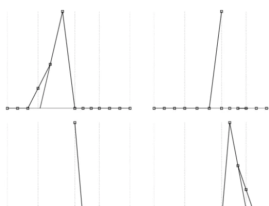
(j) 2j₋1=5.

and Manni (2010b), Proposition 8, it is proven that the functions B(_Rj_,0)

,

B(_Rj_,3) satisfy condition (4), hence the basis (30) is totally positive and can be referred to as a Bernstein basis. If we set

u(_Rj)

:=

B(_Rj_,0)

,

v(_Rj)

:=

B(_Rj_,3)

,

(31)

we observe that E

R

(j)_{has the form (1), that isE}

_R

(j)

₌

₁

_,

_x

_,

_u(j) R

,

v

(j) R

.

3.2. The space of cubic functions E

C

(j)

In the previous subsection we have seen that it is possible to apply an Hermite subdivision scheme to a rational function and obtain at level j a piecewise function with the same properties of cubic polynomials and composed by cubic pieces except in the first and last subinterval. Let us consider (31): aim of this subsection is to substitute the two rational pieces u(_Rj),v(_Rj)with cubic onesu

˜

_C(j),v

˜

(_Cj), obtaining the space E

C

(j) _ofC2 _{piecewise cubic functions with tension properties. We}

first describe the process applying a matrix transformation to a general rational net and then we explain the underlying geometric ideas detailing the construction ofv

˜

(_Cj).

Let

ξ

(j),b(j), given by (27), define the control net of a generic function

ψ

∈

E

R

(j)_{. We define}

_ξ

˜

(j)_,b

˜

(j)_as

_˜

ξ

(j)

,

b

˜

(j)

=

Σ

(j)

ξ

(j)

,

b(j)

(32)

where

Σ

(j)

_∈

_R

82j_×82j

has the form

Σ

(j)

=

⎡

⎢

⎢

⎢

⎢

⎢

⎢

⎢

⎢

⎢

⎢

⎢

⎢

⎢

⎣

1 0 0

· · ·

0 0 0

0 V

(

μ

(₀j)

)

1

−

V

(

μ

(₀j)

)

· · ·

0 0 0

0 0 1

· · ·

0 0 0

..

.

..

.

..

.

. .

.

..

.

..

.

..

.

0 0 0

· · ·

1 0 0

0 0 0

· · ·

1

−

V

(

ν

₂(jj)₋₁

)

V

(

ν

(j) 2j₋₁

)

0

0 0 0

· · ·

0 0 1

⎤

⎥

⎥

⎥

⎥

⎥

⎥

⎥

⎥

⎥

⎥

⎥

⎥

⎥

⎦

and

V

(

x

)

=

x

Note that V

(

x

) <

0, V

(

3

)

=

1, limx→∞V

(

x

)

=

1

/

2 and so

Σ

(j)defines a corner cutting matrix. Let us recall Proposition 2; since

μ

(_kj)

=

ν

_k(j)

=

3 fork

=

1

, . . . ,

2j

−

1, the points

ξ

_k(_,j_q) coincide with the control points of cubic polynomials, with the exception of the second and second last control points:

ξ

_0,1(j),

ξ

₂(jj)_−1,2. Clearly (32) implies that

˜

ξ

_k(_,j_q)

=

ξ

_k(_,j_q)

,

(

k

,

q

)

=

(

0

,

1

),

2j

−

1

,

2

and

˜

ξ

_0,1(j)

=

ξ

_0,0(j)

+

hj

3

=

hj

3

,

ξ

˜

(j) 2j_−1,2

=

ξ

(j) 2j_−1,3

−

hj 3

=

1

−

hj 3

,

withhj

=

2−j. Therefore all the components of

ξ

˜

(j)

coincide with the abscissas of the control points of cubic polynomials. Let

˜

ψ

_k(j)

(

x

)

:=

3

q=0

˜

b_k(j_,q)

3 q

(

1

−

t

)

3−qtq

,

t

=

x

−

x

(j) k hj

;

note that

ψ

˜

_k(j)

=

ψ

_k(j),k

=

1

, . . . ,

2j

₋

₂

_,

_where

_ψ

(j)

k are given in (21). Let

˜

Ψ

(j)

: ˜

Ψ

(j)

(

x

)

= ˜

ψ

_k(j)

(

x

),

x

∈

x(_kj)

,

x(_k+j)₁

,

(33)

and let

B

(_Cj)be the linear operator such that

Ψ

˜

(j)

₌

_B

(j) C b

˜

(j)

.

We define the space ofextended cubic functions

E

C

(j)

:=

Ψ

˜

(j)given in (33)

.

(34)

Note that, for any

Ψ

˜

(j)

∈

E

C

(j)_,

˜

Ψ

(j)

=

B

(_Cj)

Σ

(j)S(j)S(j−1)

· · ·

S(0)b(0)

;

(35)

moreover, using the expression for the second derivatives given in (6), it is simple to verify that

D2

ψ

˜

_k(₋j)₁ x(_kj)

=

D2

ψ

˜

_k(j) x_k(j)

that is

Ψ

˜

(j)

_∈

_C2

_[

₀

_,

₁

_]

_.

It is possible to obtain the analogous of (30):

˜

B(_Cj_,)_p

:=

B

(j)

C

Σ

(j)S(j)S(j−1)

· · ·

S(1)S(0)eTp

,

p

=

1

, . . . ,

4

.

(36)

We recall Definition 1 and state the following property.

Theorem 1.The set

{ ˜

B_C(j_,0)

,

B

˜

(_Cj_,1)

,

B

˜

(_Cj_,2)

,

B

˜

(_Cj_,3)

}

is a Bernstein basis.

Proof. Since the control nets are obtained via a corner cutting process, the functions (36) form a partition of unity and satisfy (2). Using arguments completely similar to those of Proposition 8 of Costantini and Manni (2010b), it is possible to prove that B

˜

(_Cj_,0) andB

˜

(_Cj_,3) satisfy (4) and so the basis (36) is totally positive.

2

Note that the matrix

Σ

(j) can be decomposed in the product of bidiagonal and stochastic matrices; therefore (32) defines a corner cutting process, the product of the matrices in (35) is a totally positive matrix, since it is a product of totally positive matrices, and

Ψ

˜

(j) preserves the shape of the original control polygon.

Clearly

E

C

(j)

=

B

˜

(_Cj_,0)

,

B

˜

(_Cj_,1)

,

B

˜

(_Cj_,2)

,

B

˜

(_Cj_,3)

and, if we setu

˜

(_Cj)

:= ˜

B_C(j_,0)

,

v

˜

(_Cj)

:= ˜

B(_Cj_,3)

,

then E

C

(j)_{can be written in the form (1), that is}

E

C

(j)

=

1

,

x

,

u

˜

_C(j)

,

v

˜

(_Cj)

.

(37)

Before giving further details a geometric interpretation of the matrix

Σ

(j) _{is in order. This geometric interpretation also}

allows the explicit computation of some quantities necessary for practical applications of the space E

C

(j). Since the linear process described in (35) is a corner cutting – which leaves unchanged the functions 1 andx– in view of (37) the analysis can be restricted to u

˜

(_Cj)

,

v

˜

_C(j) and, in particular, to v

˜

(_Cj) since the other is similar. The basic idea is the following: the four control points of the last rational piece at level j, namely

ξ

₂(jj)_−1,0

,

b

(j) 2j_−1,0

,

ξ

₂(jj₋)_1,1

,

b

(j) 2j_−1,1

,

ξ

₂(jj)_−1,2

,

b

(j) 2j_−1,2

,

ξ

₂(jj)_−1,3

,

b

(j) 2j_−1,3

[image:12.561.163.374.57.179.2]

Fig. 6.The modification of the 2j_{−1 rational piece.}

will be changed into

˜

ξ

₂(jj)_−1,0

,

b

˜

(j) 2j_−1,0

,

ξ

˜

₂(jj)_−1,1

,

b

˜

(j) 2j_−1,1

,

ξ

˜

₂(jj)_−1,2

,

b

˜

(j) 2j_−1,2

,

ξ

˜

₂(jj₋)_1,3

,

b

˜

(j) 2j_−1,3

,

where

˜

ξ

₂(jj)_−1,p

,

b

˜

(j) 2j_−1,p

=

ξ

₂(jj₋)_1,p

,

b

(j) 2j_−1,p

,

p

=

0

,

1

,

3

and

˜

ξ

₂(jj)_−1,2

,

b

˜

(j) 2j_−1,2

=

(

Gx

,

Gy

).

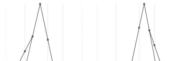
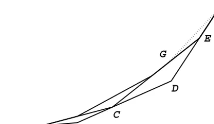
The scheme is essentially contained in Fig. 6, which shows the subdivision process from level j

−

1 to level j for the last piece in the interval

[

x(₂jj−−11)₋₁

,

x

(j−1)

2j−1

]

and should be compared with Fig. 5. For the sake of readability some of the control

points have been relabelled and, in particular,

F

=

(

Fx

,

Fy

)

=

ξ

₂(jj−−11)_−1,3

,

b (j−1) 2j−1_−1,3

=

ξ

₂(jj₋)_1,3

,

b

(j) 2j_−1,3

=

(

1

,

1

),

D

=

(

Dx

,

Dy

)

=

ξ

₂(jj−−11)_−1,2

,

b (j−1) 2j−1_−1,2

,

E

=

(

Ex

,

Ey

)

=

ξ

₂(jj₋)_1,2

,

b

(j) 2j_−1,2

,

C

=

(

Cx

,

Cy

)

is given by the application of the matrix S₂(jj)_−1,1 (see Fig. 5, top-right) and finally G

=

(

Gx

,

Gy

)

is the sought

for control point of the cubic piece. We recall that

D

=

1

−

1 2j−1

_ν

(j−1)

2j−1₋₁

,

1

−

ν

(0) 0

2j−1

_ν

(j−1) 2j−1₋₁

,

E

=

1

−

1 2j

_ν

(j)

2j₋₁

)

,

1

−

ν

(0) 0

2j

_ν

(j) 2j₋₁

)

.

Since Gx is the abscissa of the control point of a cubic polynomial Gx

=

1

−

1

/(

2j3

)

; moreover, it is simple to verify that Cx

=

(

x(₂jj−−11)₋₁

+

x

(j−1) 2j−1

)/

2. Let

Δ

(j−1)

2j−1₋₁

:=

Dy

−

Cy Dx

−

Cx

;

Δ

(j)

2j₋₁

:=

Ey

−

Cy Ex

−

Cx

(38)

and

r(₂jj−−11)₋₁

(

x

)

:=

Δ

(j−1)

2j−1₋₁

(

x

−

Cx

)

+

Cy; r (j)

2j₋₁

(

x

)

:=

Δ

(j)

2j₋₁

(

x

−

Cx

)

+

Cy; (39)

if we recall (5) we see thatr(₂jj−−11)₋₁andr (j)

2j₋₁ are, respectively, the straight lines through the second and third control points

of

ψ

₂(jj−−11)₋₁and

ψ

(j)

2j₋₁. We have the following result.

Lemma 1.Let

Δ

(₂jj)₋₁be given by(38);then

Δ

(₂jj)₋₁

=

6

1

3

(

4j

−

1

)

ν

(0)

0

−

2j

+

1

(

ν

₀(0)

+

2j+1

₋

₃

₎₍

_ν

(0)

0

+

2j

−

3

)