City, University of London Institutional Repository
Citation
:
Iori, G. and Precup, O. V. (2006). Weighted network analysis of high frequency cross-correlation measures (06/10). London, UK: Department of Economics, City University London.This is the unspecified version of the paper.
This version of the publication may differ from the final published
version.
Permanent repository link:
http://openaccess.city.ac.uk/1453/Link to published version
:
06/10Copyright and reuse:
City Research Online aims to make research
outputs of City, University of London available to a wider audience.
Copyright and Moral Rights remain with the author(s) and/or copyright
holders. URLs from City Research Online may be freely distributed and
linked to.
City Research Online: http://openaccess.city.ac.uk/ [email protected]
Department of Economics
School of Social Sciences
Weighted Network Analysis of High Frequency
Cross-Correlation Measures
Giulia Iori
1Department of Economics, City University
Ovidiu V. Precup
2Department of Mathematics, London School of Economics
Department of Economics
Discussion Paper Series
No. 06/10
1
Department of Economics, City University, Northampton Square, London, EC1V
0H
B
, UK. Email: [email protected]
2
Department of Mathematics, London School of Economics, Houghton Street,
Weighted Network Analysis of High Frequency
Cross-Correlation Measures
Giulia Iori∗
Department of Economics, City University Northampton Square London, EC1V 0HB, U.K.
E-mail: [email protected]
Ovidiu V. Precup
Department of Mathematics, London School of Economics Houghton Street, London, WC2A 2AE, U.K.
E-mail: [email protected]
October 25, 2006
Abstract
In this paper we implement a Fourier method to estimate high frequency correlation matrices from small data sets. The Fourier estimates are shown to be considerably less noisy than the standard Pearson correlation measure and thus capable of detecting subtle changes in correlation matrices with just a month of data. The evolution of correlation at different time scales is analysed from the full correlation matrix and its Minimum Spanning Tree representation. The analysis is performed by implementing measures from the theory of random weighted networks.
Keywords: High-Frequency Correlation, Fourier method, random weighted networks.
1
Introduction
Robust correlation measures are important for derivatives pricing, risk management, portfolio optimisation and for understanding market microstructure effects.
The conventional method of computing correlation is the Pearson coefficient. This method requires homogeneous time series and in order to apply it to high frequency data, the time series need to be homogenised and synchronised first through an interpolation scheme.
An alternative, non parametric approach has been suggested in [1] where the variance-covariance matrix estimator of a multivariate process is computed via Fourier analysis. Previ-ous applications of the method can be found in [2, 3, 4, 5, 6, 7].
In this paper we compare the performance of the Pearson and Fourier methods by computing returns cross-correlation matrices at different time scales using one month (September 2002) of high frequency trades in the member stocks of the S&P1001 index.
The selected stocks are grouped into twelve different industry sectors2: Technology (16
∗Corresponding author
1data source: NYSE Trades and Quotes (TAQ) database
stocks), Basic Materials (7 stocks), Financial (13 stocks), Capital Goods (3 stocks), Conglom-erates (5 stocks), Energy (4 stocks), Services (16 stocks), Transport (4 stocks), Utilities (7 stocks), Health Care (10 stocks), Non-Cyclical Consumer Goods (11 stocks), Cyclical Con-sumer Goods (4 stocks).
The estimation of intra-day correlations over short periods of time (eg. a month) is of high practical value for day trading and hedging purposes. In fact, such estimates are more sensitive to short timescale economic changes than correlation measures obtained from averaging over several months. Thus, we choose to investigate a month of tick-by-tick data aiming to compare the quality of the information that can be derived by applying each of the two methods on lim-ited statistics. The Fourier estimates reproduce the structural changes on filtered correlation matrices observed in previous studies [8, 9, 10, 11, 12, 13, 14, 15, 16] with much larger data sets. Moreover, we show that the Fourier estimates are sufficiently accurate to reveal further structural changes in the full, unfiltered, correlation matrices.
2
Fourier Correlation Measure
The Fourier method is model independent, produces very accurate, smooth estimates and handles the time series in their original form without imputation or discarding of data. A rigorous proof of the method is given in the original paper by Malliavin and Mancino[1] and only the main results are summarized below.
The method works as follows. Let Si(t) be the price of asset i at time t and pi(t) =
lnSi(t). The physical time interval of the asset price series is re-scaled to [0,2π]. The
vari-ance/covariance matrix Σij of log returns is derived from its Fourier coefficient a0(Σij) which is obtained from the Fourier coefficients of dpi:
ak(dpi) = π1
2π
0 cos(kt)dpi(t), bk(dpi) =
1
π
2π
0 sin(kt)dpi(t), k≥1. (1)
In practice, the coefficients are computed through integration by parts. As pi(t) is not
observed continuously but given by unevenly spaced tick-by-tick observations of trades prices, the actual implementation requires the integrals in (1) to be in discrete form:
ak(dpi) = 1
π N
n=1
[pi(tn) cos(ktn)−pi(tn) cos(ktn)]−pi(tn)[cos(ktn)−cos(ktn)]
,
bk(dpi) = 1
π N
n=1
[pi(tn) sin(ktn)−pi(tn) sin(ktn)]−pi(tn)[sin(ktn)−sin(ktn)]
. (2)
where tn=tn−1
In (2),N corresponds to the number of trades in the re-scaled interval and we set the price
pi(t) =pi(tn−1) to compute the integrals between two consecutive trading times [tn−1, tn].
The Fourier coefficient of the pointwise variance/covariance matrix Σij is :
a0(Σij) = limτ→0πτ T
T/2τ
k=1
[ak(dpi)ak(dpj) +bk(dpi)bk(dpj)]. (3)
The integrated value of Σij over the time window is defined as ˆσ2ij = 2πa0(Σij) which leads to the Fourier correlation matrixρij = ˆσij2/(ˆσii·σˆjj).
0 20 40 60 80 100 120
time scale 0.2
0.25 0.3 0.35 0.4 0.45
[image:5.595.155.402.149.333.2]average correlation
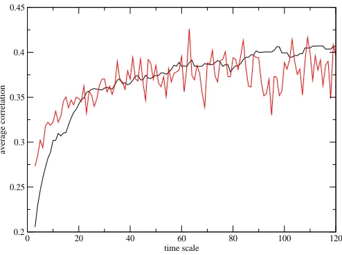
Figure 1: The average correlation across all stocks increases with time scale (Fourier (black) and Pearson (red)). This is indicative of the Epps affect being present.
3
Network Analysis
The correlation matrix can be represented as a network of vertices (stocks) and weighted links (correlations). Following [17, 18] we define the degree of a vertex in the network as
ki =j∈V(i)1ij where the sum runs over the setV(i) of neighbours ofiand 1ij is an indicator function for whether there is a connection between iand j. Thestrength of a vertex is defined as si =j∈V(i)cij where cij is the correlation between vertices (stocks) iand j. We use the
degree ki as a measure of stock centrality for MSTs and the strength si as a measure of stock
centrality in the overall correlation matrices. For the weighted clustering coefficient we use the definition suggested in [19],
Ciw =
j,hcijcihcjh
j,hcijcih .
(4)
This definition reduces to the standard clustering coefficient in the binary case and retains the property 0≤CiW ≤1.
For our analysis we only consider the positive elements of the correlation matrices. Even with this choice the correlation matrix is almost fully connected.
When analysing intra-day data, the choice of time scale on which to measure correlations becomes crucial. In Figure 1 we plot the average correlation at different time scales, from three minutes to two hours. The average correlation increases with the time scale, a result known as the Epps effect [20] 3. Not only does the average correlation increase with time scale, but it is also accompanied by a structural change in the correlation matrix as shown in [8, 9, 10, 11, 12, 13] and more recently, using the Planar Maximally Filtered Graph method
3It has been argued [4, 6] that the Epps effect may be determined not purely by economic factors but also
1 2 3 4 5 6 7 8 9 10 11 12 13 14 15 16 17 18 19 20 21 22 23 24 25 26 27 28 29 30 31 32 33 34 3536 37 38 39 40 41 42 43 44 45 46 47 48 49 50 51 52 53 54 55 56 57 58 59 60 61 62 63 64 65 66 67 68 69 70 71 72 73 74 75 76 77 78 79 80 81 82 83 84 85 86 87 88 89 90 91 92 93 94 95 96 97 98 99 100 1 2 3 4 5 6 7 8 9 10 11 12 13 14 15 16 17 18 19 20 21 22 23 24 25 26 27 28 29 30 31 32 34 35 36 37 38 39 40 41 42 43 44 45 46 47 48 49 50 51 52 53 54 55 56 57 58 59 60 61 62 63 64 65 66 67 68 69 70 71 72 73 74 75 76 77 78 79 80 81 82 83 84 85 86 87 88 89 90 91 92 93 94 95 96 97 98 99 100
Figure 2: MST obtained with Fourier at 10 minutes (left) and 90 minutes (right). WMT is node 97 and GE is node 39. The size of the dots reprenting the different socks is proportional to the number of links. The color code of the different industrial sectors is given in table 3.
0 20 40 60 80 100
time scale 5 10 15 20 25
degree of the most connected stock
0 20 40 60 80 100 120
time scale 0 5 10 15 MST degree
Figure 3: (Left) Degree of the most connected stock in the MST for Fourier (black) and Pearson (red). (Right) Degree of GE (black) and WMT (red) as a function of the time scale (Fourier).
[image:6.595.72.487.403.566.2]Method average degree Stock 7.36 Wal-Mart Stores Fourier 5.94 General Electric 5.43 Boise Cascade 4.65 Americal Express
4.57 Intel Corp
10.36 Wal-Mart Stores
Pearson 8.40 US Bancorp
6.89 Bank of America 5.25 Exxon Mobil Corp
[image:7.595.162.396.69.223.2]5.07 Intel Corp.
Table 1: Vertices with the highest average degree in the MST on time scales shorter than 30 minutes.
To quantify the structural change of the MST in figure 3 (left) we plot the evolution, up to a two hours time scales, of the degree of the most connected vertex in the MST derived from both Pearson(red) and Fourier(black) correlation estimates. We notice that while the Pearson estimate gives very noisy results on this small data set (also visible in Figure 1), the Fourier estimator provides much more consistent results across different time scales. In Table 1 we list the five most connected stocks in the MST generated with the two methods. In [15] General Electric (GE) and Wal-Mart (WMT) are reported as the most connected stocks in 2002. When averaging up to time scales of 30 minutes, we find WMT to be the stock with the highest average degree for September 2002. This result is not affected by the method used to estimate correlations. Nonetheless, the Fourier and Pearson methods results differ when it comes to identifying the remaining most connected stocks in the MST. For example while Fourier identifies GE to be the second most connected stock, Pearson ranks GE as the eighth most connected one. Figure 3 (right) shows the evolution of the maximum degree for WMT and GE obtained from the Fourier MST matrix. For both stocks the degree rises quickly and remains high at time scales between 10 and 20 minutes. Nonetheless at time scales longer than 20 minutes, and up to two hours, WMT is the most connected stock in the MST.
To analyze the full correlation matrix we implement the measures of strengths and clus-tering defined above. While some analysis in this direction has been performed in previous studies, this was based on filtered correlation matrix (either planary filtered graphs [14, 15, 16] or graphs constructed by including only the strongestN−1 links, withN the number of stocks [11]).
In Figure 4 (left) we plot the evolution, across time scales, of the normalised strength of the most connected vertex in the full correlation matrix calculated both with Pearson (red) and Fourier (black). The normalised strength, at any time scale τ is defined as ˜si(τ) =si(τ)/ˆc(τ), where ˆc(τ) is the scale τ total correlation. Without this normalisation the strength would trivially increase with time scale as a result of the Epps effect. By normalising we can quantify the way the most correlated stock is central to the network, in terms of proportional contri-bution to the total correlation. We notice again (Figure 4 (left)) that the Pearson estimator is very noisy while the Fourier estimator is significantly smoother. The Fourier estimator also indicates a rise in the most correlated stocks relative strengths, at time scales shorter than 20 minutes, analogous to the increasing degree of the most connected stock in the MST on short time scales.
0 20 40 60 80 100 120 time scale
0.0125 0.013 0.0135 0.014 0.0145
normalized strength
0 20 40 60 80 100 120
time scale 0.011
0.0115 0.012 0.0125 0.013 0.0135 0.014
normalized strength
Figure 4: (Left) Normalised strength of the most correlated stock determined with the Fourier (black) and Pearson (red) methods. (Right) Fourier normalised strength of GE (black) and WMT (red) as a function of time scale (Fourier).
WMT is the most central stock at all time scales up to two hours.
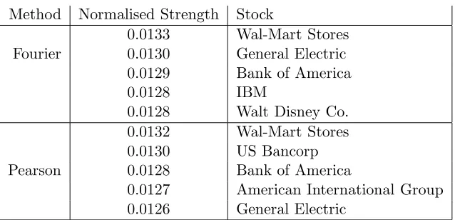
Method Normalised Strength Stock
0.0133 Wal-Mart Stores
Fourier 0.0130 General Electric
0.0129 Bank of America
0.0128 IBM
0.0128 Walt Disney Co. 0.0132 Wal-Mart Stores
0.0130 US Bancorp
Pearson 0.0128 Bank of America
[image:8.595.71.488.97.264.2]0.0127 American International Group 0.0126 General Electric
Table 2: Vertex with highest average normalised strength at time scales shorter than 30 minutes
In Figure 5 (left) we plot the evolution, across time scales, of the the relative weighted clustering coefficient of the most clustered stock in the full correlation matrix calculated both with Pearson (red) and Fourier (black). The relative weighted clustering coefficient is defined as ˜Ciw(τ) = Ciw(τ)
¯
Cw(τ), where ¯Cw(τ) is the scaleτ average clustering coefficient. The normalisation
[image:8.595.120.439.366.520.2]highly correlated with each other. This effect is particularly evident for the Cyclical Consumer Goods and the Capital Goods sectors.
0 20 40 60 80 100 120
time scale 1.05
1.06 1.07 1.08 1.09 1.1 1.11 1.12
[image:9.595.155.399.138.302.2]relative clustering
Figure 5: Relative clustering coefficient of the highest cluster coefficient stocks - Fourier (black) and Pearson (red).
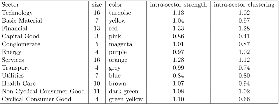
The most clustered sector at all time scales, up to two hours, is the Financial one. At short time scales this is followed by Services, Technology, Energy, and Non-Cyclical Consumer Goods. The study in [15] uses the same sector classification but a different selection of stocks (100 highly capitalised stocks instead of the member stocks of the S&P100) and finds that the Financial and the Energy sectors have the highest intra-sectors cluestering, on planary filtered graphs, on a daily time scale. This is in agreement with our results, even though we only include 13 stocks in the Financial sector while in [15] 24 stocks are selected.
Sector size color intra-sector strength intra-sector clustering
Technology 16 turqoise 1.13 1.02
Basic Material 7 yellow 1.04 0.97
Financial 13 red 1.33 1.28
Capital Good 3 pink 0.86 0.41
Conglomerate 5 magenta 1.01 0.87
Energy 4 purple 0.97 1.02
Services 16 orange 1.28 1.12
Transport 4 grey 0.99 0.74
Utilities 7 blue 0.84 0.80
Health Care 10 brown 1.07 0.94
Non-Cyclical Consumer Good 11 dark green 1.08 1.02
Cyclical Consumer Good 4 green yellow 1.10 0.66
Table 3: Intra-sector relative strength and clustering coefficients at time scales shorter than 30 minutes.
[image:9.595.58.536.468.649.2]0 20 40 60 80 100 120 140 160 180 200 time scale
0.8 1 1.2 1.4
relative sector clustering
[image:10.595.146.412.96.284.2]Technology Basic Material Financial Energy Services Health Services Non Cyclical CG
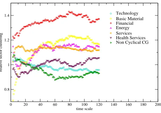
Figure 6: Relative clustering coefficient of the five most clustered industrial sectors.
present). Another possible reason may be the difference in time scale at which the correlations are measured. In Figure 6 we plot the relative clustering coefficient for the 7 most clustered sectors as a function of the time scale. We can see that the ranking of sectors in terms of their relative clustering coefficients changes considerably over time, and in particular the Services sector, which is the second most clustered at short time scale, becomes only the fourth most clustered on two hours time scales. It may well be that that the relative clustering of this sector decreases even further on daily time scales.
The high clustering coefficient of some sectors is reflected in the MST. For example, the MST at 10 minutes in figure 2 (left), identifies very clearly the clusters associated to the Finan-cial (red), Services (orange), Non-cyclical consumer good (green), and Technology (turquoise) sectors. On the contrary at 90 minutes both the Service and Non-Cyclical Consumer Good clusters are broken while in addition to the the Financial and technology, also the Basic Ma-terial sector (the second most clustered sector at this time scale) is perfectly identified.
4
Conclusions
The analysis carried out in this paper provides further evidence that the Fourier method of computing the correlation matrix from high-frequency data is better than the traditional Pearson alternative in terms of generating smooth, robust estimates from small sample data sets.
most intra-connected at all time scales up to two hours.
5
Acknowledgements
We are very grateful to Roberto Ren`o, Vanessa Mattiussi, Anirban Chakraborti and Rosario Mantegna for stimulating discussions.
References
[1] Malliavin P, Mancino M (2002) Fourier series method for measurement of multivariate volatilities, Finance & Stochastics 6(1), 49-61.
[2] Barucci E, Ren`o R (2002) On measuring volatility and the GARCH forecasting perfor-mance, Journal of International Financial Markets, Institutions and Money, 12 182-200.
[3] Barucci E, Ren`o R (2002) On measuring volatility of diffusion processes with high fre-quency data, Economics Letters 74, 3(2) 371-378.
[4] Ren`o R (2003) A closer look at the Epps effect, International Journal of Theoretical and Applied Finance, 6 (1), 87-102.
[5] Precup O V, Iori G, (2004) A Comparison of High-Frequency Cross-Correlation Measures, Physica A, Vol 344/1-2, 252-256.
[6] Precup O V, Iori G, (2007) Cross-correlation in the high-frequency domain, European Journal of Finance (forthcoming).
[7] Mattiussi V, Iori G, (2007) ”Currency futures volatility during the 1997 East Asian crisis: an application of Fourier analysis”, Chapter 5 in B.A. Goss (ed), Debt, Risk and Liquidity in Futures Markets, London and New York: Routledge (forthcoming).
[8] Bonanno G, Lillo F, Mantegna R N, (2001) High-frequency Cross-correlation in a Set of Stocks, Quantitative Finance 1, 96-104.
[9] Bonanno G, Caldarelli G, Lillo, Mantegna R N, (2002) Topology of correlation based minimal spanning trees in real and model markets, Physical Review E 68, 046130.
[10] Bonanno G, Caldarelli G, Lillo F, Miccich`e S, Vandewalle N, Mantegna R N (2004) Net-works of equities in financial markets, The Eur. Phys. J. B 38, 363-371.
[11] Onnela J-P, Chakraborti A, Kaski K, Kertesz J, Kanto A (2003) Asset trees and asset graphs in financial markets, Physica Scripta Online Vol. T106, 48.
[12] Onnela J-P, Chakraborti A, Kaski K, Kertesz J (2003) Dynamic asset trees and Black Monday, Physica A 324, 247-252.
[13] Onnela J-P, Kaski K, Kertesz J (2004) Clustering and information in correlation based financial networks, Eur. Phys. J. B Vol. 38 No. 2, p.353.
[14] Tumminello M, Aste T, Di Matteo T, Mantegna R N, Proc. Natl. Acad. Sci. USA 102, no. 30,10421-10426 (2005) .
[16] Tumminello M, Di Matteo T, Aste T, Mantegna R N, Correlation based networks of equity returns sampled at different time horizons.
[17] Barrat A, Barth´elemy M, Vespignani A, (2004), Weighted evolving networks: coupling topology and weights dynamics, Phys. Rev. Lett.92 228701.
[18] Newman M E J, (2004), Analysis of weighted networks, Phys. Rev. E 70, 05613.
[19] Kalna G, Higham D J, Clustering Coefficients for Weighted Networks