ESTIMATION OF MINKOWSKI TENSORS FROM DIGITAL GREY-SCALE IMAGES

ESTIMATION OF MINKOWSKI TENSORS FROM DIGITAL GREY-SCALE

IMAGES

A

M

S

Karlsruhe Institute of Technology, Institute of Stochastics, D-76128 Karlsruhe, Germany e-mail: [email protected]

(Received January 30, 2014; revised July 23, 2014; accepted July 25, 2014)

ABSTRACT

It was shown in Svane (2014b) that local algorithms based on grey-scale images sometimes lead to asymptotically unbiased estimators for surface area and integrated mean curvature. This paper extends the results to estimators for Minkowski tensors. In particular, asymptotically unbiased local algorithms for estimation of all volume and surface tensors and certain mean curvature tensors are given. This requires an extension of the asymptotic formulas of Svane (2014b) to estimators with position dependent weights. Keywords: digital stereology, grey-scale images, local algorithms, Minkowski tensors.

INTRODUCTION

Minkowski tensors (Schneider and Schuster, 2002; Huget al., 2008) are generalisations of Minkowski functionals (Matheron, 1975; Schneider, 1993). They associate to a compact convex body X ⊆ Rd a

symmetric tensor, rather than a scalar. They carry information about shape features ofXsuch as position, anisotropy, and eccentricity. For this reason they are used as shape descriptors in statistical physics. For instance, in Schr¨oder-Turket al. (2010b), Minkowski tensors are used to detect anisotropy in spherical bead packs (see also Schr¨oder-Turket al. (2011) for an overview).

Since the data is often of digital nature, there is a need for fast digital algorithms to estimate tensors. In the special case of Minkowski functionals, local algorithms are often chosen for this (Klette and Rosenfeld, 2004) since they can be implemented based on a linear filtering of the image (Ohser and M¨ucklich, 2000). The input is a black-and-white image, typically a thresholded grey-scale image. The idea is to count the number of times each n× · · · ×n configuration of black and white pixels occurs in the image and estimate the Minkowski functional by a weighted sum of configuration counts.

Since Minkowski tensors generally depend on the position of the underlying object, a local algorithm for these tensors would need to take the position of each n× · · · ×nconfiguration into account. Such modified algorithms are suggested in Schr¨oder-Turket al.(2008; 2010a).

It is well known that local algorithms for Minkowski functionals based on black-and-white images are generally biased (Kampf, 2012; Svane,

2014a), even when the resolution goes to infinity. The situation seems to be the same for most Minkowski tensors. For this reason, and because most black-and-white images arise as thresholded grey-scale images, local algorithms based directly on grey-scale images without thresholding were suggested in Svane (2014b) for Minkowski functionals. The existence of asymptotically unbiased algorithms for surface area and integrated mean curvature in this situation was also shown. In fact, only 1× · · · ×1 configurations are needed for this.

The purpose of this paper is to extend the results to prove the existence of asymptotically unbiased estimators for surface and mean curvature tensors as well. Larger n× · · · ×n configurations are needed for this in order to gain information about surface normals. Moreover, position dependent weights are necessary in order to get information about position.

The paper is organised as follows: We first describe the model for grey-scale images we shall be working with along with the generalised definition of local algorithms based onn× · · · ×nconfigurations of grey-values. In the next section, we show a slight extension of the known theoretical results about the asymptotic behaviour of local algorithms, which is required for the study of these algorithms. This follows fairly easily from the technical lemmas in Svane (2014b).

we obtain a complete set of estimators for the Minkowski tensors in 2D. The algorithms require that the PSF is known; at least the knowledge of what a blurred halfspace looks like is required. Moreover, the resolution has to be sufficiently high compared to the support of the PSF. Finally, we show by an example case how the formulas can be used to estimate all rank 2 tensors in 2D.

It should be emphasised that the focus of this paper is only theoretical. We construct algorithms for estimation of Minkowski tensors and show convergence in an idealised setting. It is to our best knowledge the first algorithm based on grey-scale images without thresholding and the first to come with a convergence proof. Whether these algorithms perform well in finite, but high, resolution, or when the digitisation model is only approximately valid, will be the aim of future research, see also the discussion section at the end of the paper.

LOCAL ESTIMATORS FOR

GREY-SCALE IMAGES

GREY-SCALE IMAGES

LetX⊆Rd be the compact set we are observing.

We assume that the light coming from each point is spread out following a point spread function (PSF) which is independent of the position of the point. Hence the light that reaches the observer is given by the intensity function

θX :Rd→[0,1],

where the intensity measured atx∈Rdis given by

θX(x) =

Z

X

ρ(x−z)dz.

In other words, θX is the convolution 1X ∗ρ of the

indicator function1X forX with a PSFρ. The PSF is

assumed to be a measurable function satisfying

(i) ρ≥0 .

(ii) R

Rdρ(z)dz=1 .

We say that a PSF is rotation invariant ifρ(x) =ρ(|x|) depends only on|x|.

A digital grey-scale image is the restriction ofθX to an observation lattice L. A change of resolution

corresponds to a change of lattice from L to aL for

some a > 0. We assume that the precision of the measurements changes with resolution in such a way that the PSF corresponding toaLis

ρa(x) =a−dρ(a−1x),

see the discussion in Svane (2014b) Section 2.1. The corresponding intensity function is denoted

θaX(x) =

Z

X

ρa(x−z)dz=a−d

Z

X

ρ(a−1(x−z))dz.

In applications, the PSF is typically the Gaussian function (K¨othe, 2008) or the Airy disk (Airy, 1835). Another important example is ρB = Hd(B)−11B

where B ⊆ Rd is a compact set of non-zero finite

volumeHd(B). In this case, we measure at eachz∈L

the fraction of z+B covered byX. Such PSF’s have compact support, but are not continuous.

A BLURRED HALFSPACE

Foru∈Sd−1andα∈R, write

H_α,−_u={x∈Rd| hx,ui ≤α}

for the halfspace. The intensity function associated to a halfspace in standard resolution will play a special role in the following. Hence we introduce the separate notation

θu(t):=θ

H₀−_,u

1 (tu).

Note for later that

θ

H₀−_,u

a (ax) =θ H₀−_,u

1 (hx,uiu) =θu(hx,ui),

independently ofa.

Example 1. Ifρis the standard Gaussian

ρ(x) = (2π)−d2_e− 1 2|x|2,

then

θu(t) =

Z

u⊥ Z 0

−∞

ρ(tu−z−su)dsdz=Φ(−t),

where Φis the distribution function for the standard

1-dimensional normal distribution.

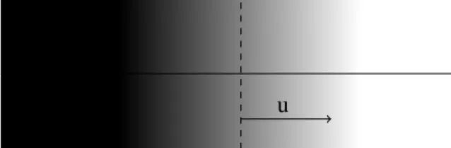
A geometric interpretation of θu is illustrated in

Fig. 1.

u

Fig. 1.A grey-scale image of a halfspace. The function

θu measures how the grey-values change along the

LOCAL ALGORITHMS IN THE GREY-SCALE SETTING

Let L be a lattice in Rd spanned by the ordered

basis v1, . . . ,vd ∈ Rd and let Cv = Ldi=1[0,vi) be

the fundamental cell of the lattice where ⊕ denotes Minkowski addition, see (Matheron, 1975). As we shall later be scaling the lattice, we may as well assume that the volume det(v1, . . . ,vd) ofCv is 1. Forc∈Rd,

we letLc=L+cdenote the lattice translated bycand

aLcthe scaling ofLcbya>0.

Fixw∈L. A fundamentaln× · · · ×nlattice block

isC_wn_,0 = (w+nCv)∩L. More generally we consider

its translationsC_wn_,z=z+Cn_w,0byz∈Rd. We denote by

[0,1]Cnw,0 _{the set ofn}d_{-tuples of points in[0,1]indexed} byCn_w,0. A point in[0,1]Cwn,0 _{is written {θ}

s}s∈Cn w,0. The restriction ofθaX toaCwn,z naturally defines a point in [0,1]Cnw,0 _{which we denote by}

ΘXa(az;aC n

w,0):={θ

X

a(az+as)}s∈Cn w,0.

Definition 2. A local algorithmΦˆqf is an estimator of

the form

ˆ

Φ_qf(X) =aq

_∑

z∈Lc

f(ΘX_a(az;aC_wn_,0),az), (1)

where f :[0,1]Cwn,0_×Rd _{→Ris a Borel function. We}

assume that the support of f is contained in A×Rd

where A⊆(0,1)Cnw,0 _{is compact and that f is bounded} on compact sets.

The assumptions on f make the sum in Eq. 1 finite andz7→ f(ΘXa(az;aCwn,0),z)integrable wheneverX is

compact.

We assume that the lattice is stationary random, i.e., we consider the lattice Lc=L+c where c∈Cv

is uniform random. Then the mean estimator is

EΦˆqf(X) =a q

E

_∑

z∈_Lc

f(ΘXa(az;aC n

w,0),az) (2)

=aq−d

Z

Rd

f(ΘX_a(z;aCwn,0),z)dz.

As a natural convergence criterion, we take the following:

Definition 3. A local algorithm Φˆqf(X) is called

an asymptotically unbiased estimator for Φ(X) if

lima→0EΦˆ

f

q(X) =Φ(X).

THE RELEVANT SET-CLASSES

In order to prove the formulas, we need to make some assumptions on X. First some notation. For a closed set X ⊆Rd, we let exo(X) denote the points

in Rd not having a unique nearest point in X. Let

ξX :Rd\exo(X)→Xbe the natural projection taking a

point inRd\exo(X)to its nearest point inX. We define

the normal bundle ofX to be the set

N(X) = x,_|z−x|z−x ∈X×Sd−1|

z∈Rd\(X∪exo(X)),ξX(z) =x .

For(x,u)∈N(X)we define the reach

δ(X;x,u) =inf{t≥0|x+tu∈exo(X)}>0.

Let Hk denote the k-dimensional Hausdorff measure. Following Kiderlen and Rataj (2007), we introduce the class of gentle sets:

Definition 4. A closed set X⊆Rdis called gentle if:

(i) Hd−1(N(∂X)∩(B×Sd−1))<∞for any bounded Borel set B⊆Rd.

(ii) ForHd−1-almost all x∈∂X there exist two balls

Bin,Bout ⊆ Rd both containing x and such that

Bin⊆X ,int(Bout)⊆Rd\X .

The condition (ii) in the definition means that for a.a. x ∈ ∂X there is a unique pair (x,u(x)) in N(X)with(x,u(x)),(x,−u(x))∈N(∂X). This class is quite general, including for instance allC1 manifolds and all polyconvex sets satisfying a certain regularity condition (Kiderlen and Rataj, 2007).

We shall also consider the subclass of r-regular sets:

Definition 5. A gentle set X⊆Rd is called r-regular

for some r>0, if the balls Binand Bout exist for every

x∈∂X and can be chosen to have radius r.

Beingr-regular is slightly weaker than being aC2 manifold.

It can be proved (Federer, 1959), that if X is

r-regular, then ∂X is a C1 manifold with Hd−1

-a.e. differentiable normal vector field u. Thus its principal curvaturesk₁, . . . ,kd−1, corresponding to the

orthogonal principal directions e1, . . . ,ed−1 ∈ T∂X where T∂X is the tangent bundle, can be defined a.e. as the eigenvalues of the differential du. Hence the second fundamental form IIx on the tangent space

Tx∂X is defined forHd−1-a.a. x∈∂X. For a tangent

vector ∑d−i=11αiei ∈ Tx∂X, IIx is the quadratic form

given by

IIx d−1

∑

i=1

αiei !

= d−1

∑

i=1

whenever dxu is defined. In particular, the trace is

Tr(II) =k1+· · ·+kd−1. Note for later thatr-regularity

ensures thatk1, . . . ,kd−1≤r−1.

The(d−2)nd curvature measure of X is defined (Federer, 1959) forr-regular sets by

Cd−2(X;A) =

1 2π

Z

∂X∩A

Tr(II)dHd−1

for all Borel setsA⊆Rd.

ASYMPTOTIC FORMULAS

FIRST ORDER FORMULAS

The following notation will be used in the proofs. For a finite setS,|S|denotes the cardinality ofS. Given an intervalI, we denote byISthe|S|-tuples{θs}s∈S of

points θs∈I indexed by S. Given a finite setS⊆Rd

we write

ΘX_a(x;S) ={θ_aX(x+s)}s∈S∈[0,1]S,

Θu(t;S) ={θu(t+hs,ui)}s∈S∈[0,1]S.

Forx∈∂X understood anduan outward pointing normal, we also writeHu:=H_hx−_,ui,ufor the supporting

halfspace. Note that

θaHu(x+a(tu+s)) =θ H₀−_,u

a (a(t+hs,ui)u) =θu(t+hs,ui)

Θu(t;S) ={θaHu(x+a(tu+s))}s∈S.

The proofs follow from the following lemma shown in Svane (2014b), Lemma 7.1 and 7.2:

Lemma 6. Suppose X is gentle and ρ is a bounded

PSF. Let D>0. Then for a.a. x∈∂X ,

lim

a→0sup{|θ

X

a(x+atu+as)−θu(t+hs,ui)|,

t∈[−D,D],s∈B(D)}=0,

where B(D)denotes the ball inRdof radius D.

Theorem 7. Suppose X ⊆ Rd is a compact gentle

set, S ⊆Rd is finite, and ρ is a bounded PSF. Let

f :(0,1)S×Rd →Rbe continuous and assume that

supp f ⊆[β,ω]S×Rd for someβ,ω∈(0,1). Then

lim

a→0a

−1Z

Rd

f(ΘXa(x;aS),x)dx

=

Z

∂X

Z

R

f(Θu(t;S),x)dtHd−1(dx).

Proof. LetD>0 be such that

Z

|x|≥D

2

ρ(x)dx≤β∧(1−ω),

andS⊆B D₂. This ensures that

suppf(ΘXa(x;aS),x)⊆∂X⊕B(aD).

Then the generalized Weyl tube formula in Huget al. (2004), Theorem 2.1, yields

Z

Rd

f(ΘXa(x;aS),x)dx= d

∑

m=1

mκm

Z

N(∂X)

Z δ(∂X;x,u)

0

tm−1f(ΘXa(x+tu;aS),x+tu)dtµd−m(∂X; d(x,u)).

(3)

Hereκm is the volume of the unit ball in Rm and the

µi are certain signed measures of locally finite total

variation.

Observe that

Z δ(∂X;x,u)

0

tm−1f(ΘXa(x+tu;aS),x+tu)dt

≤m−1amDmsup|f|, (4)

so that dominated convergence together with Kiderlen and Rataj (2007), Eq. 8 yields

lim

a→0a

−1

d

∑

m=1

mκm

Z

N(∂X)

Z aD

0

tm−1

f(ΘXa(x+tu;aS),x+tu)dtµd−m(∂X; d(x,u))

=

Z

∂X

lim

a→0

Z D

−D

f(ΘX_a(x+atu;aS),x+atu)dt

Hd−1_(dx)

=

Z

∂X

Z D

−D

f(Θu(t;S),x)dtHd−1(dx).

The last equation follows from Lemma 6 and continuity of f.

Assume X is compact gentle andρ bounded. Let A ⊆ (0,1)S _{be a compact set and g :}

Rd → R a

continuous function. Define the measures onA given for any Borel setB⊆Aby

µ_aX,g(B) =a−1

Z

Rd

1B ΘXa(x+atu;aS)

g(x)dx,

and

µX,g(B) =

Z

∂X

Z D

−D1B Θu(t;S)

Corollary 8. Let X be a compact gentle set and

let A⊆ (0,1)S a compact set. Let g : Rd → R be

continuous and assume µX,g(∂A) = 0. Then µaX,g

converges weakly toµX,g. In particular, if h:A→R

is continuous and f(Θ,x) =h(Θ)g(x), then

lim

a→0E

ˆ

Φqf(X) =

Z

∂X

Z D

−D

h(Θu(t;S))dt g(x)Hd−1(dx).

Proof. For any bounded continuoush:A→R,

Z

A

hdµaX,g→

Z

A

hdµX,g.

This follows from Theorem 7 by approximatinghby continuous functions on(0,1)S_.

NOTATION

We next introduce some more notation that will be used in order to keep formulas short in the statement of the main second order theorem and its proof. Moreover, we state a technical lemma proved in Svane (2014b).

We will assumeρto be continuous and compactly supported. In this case allθuareC1with(u,t)7→θu0(t)

continuous. We say thatβ ∈(0,1)is a regular value if θu0(t)<0 for allt with θu(t) =β and all u∈Sd−1.

Since θu is decreasing, this ensures that θu−1(β) is

uniquely determined.

For X ⊆ Rd r-regular, define the quadratic

approximationQx toXatx∈∂X by

Qx={z∈Rd | hz−x,ui ≤ −1₂IIx(πu⊥(z−x))}

whereπ_u⊥:_Rd→u⊥ denotes orthogonal projections.

It is shown in Svane (2014b), in the proof of Lemma 7.6, that fors∈Rd

θ_aQx(x+a(tu+s)) =θu(t+hs,ui) +aθQx_{(t,s) +o(a)}

(5) where

θQx(t,s) =−1 2

Z

u⊥

IIx(z)ρ(tu+s−z)dz.

Again we use the notation

ΘQax(t;S) ={θ Q_x

a (x+atu+s)}s∈S,

ΘQx(t;S) ={θQx(t,s)}s∈S.

Choose D as in the proof of Theorem 7. Given A⊆(0,1)Sandx∈∂X, let

t₀S=inf{t∈[−D,D]|Θu(t;S)∈A},

t₁S=sup{t∈[−D,D]|Θu(t;S)∈A},

t₀S(a) =inf{t∈[−D,D]|ΘQax(t;aS)∈A},

t₁S(a) =sup{t∈[−D,D]|ΘQax(t;aS)∈A},

t₀X,S(a) =inf{t∈[−D,D]|ΘXa(x+atu;aS)∈A},

t₁X,S(a) =sup{t∈[−D,D]|ΘX_a(x+atu;aS)∈A}.

Finally, let

ψ₀S(x) = max

− θ

Qx_(tS

0,s)

θu0(t0S+hs,ui)

|s∈S,t₀S=t₀s

,

ψ₁S(x) = min

− θ

Q_x(tS

1,s)

θu0(t1S+hs,ui)

|s∈S,t₁S=t₁s

.

Lemma 9. Suppose that X is r-regular and ρ is

continuous with compact support. Let R >0 and a

finite set S⊆Rdbe given.

For all a sufficiently small, t7→θaX(x+a(tu+s))

and t 7→θaQx(x+a(tu+s)) are decreasing functions

for all x∈∂X , s∈S, and t∈[−R,R].

There is a constant M>0 such that for ν=0,1 and a sufficiently small

sup

n Θ

X

a(x+atu;aS)−Θu(t;S)

, (6)

x∈∂X,t∈[−R,R]o≤Ma,

sup

n t

X,S

ν (a)−t

S

ν

|x∈∂X o

≤Ma. (7)

Assume that A=

×

all points in ∂Is are regular values. Then for each

x∈∂X andν=0,1,

sup

n Θ

X

a(x+atu;aS)−Θ Q_x a (t;aS)

|t∈[−R,R] o

,

t

X,S

ν (a)−t

S

ν(a)

, (8)

are of order o(a)and

t_νS(a) =t_νS+aψ_νS(x) +o(a). (9)

Proof. The lemma is essentially proved in Svane

(2014b). Note that the notation is changed. The first statement is proved in Lemma 7.5 for θX. The proof forθQx _{is similar. Eqs. 6 and 7 are shown in the proof}

SECOND ORDER FORMULAS

Theorem 10. Suppose X is an r-regular set andρ is

continuous and compactly supported. Let S⊆Rd be a

finite set and A=

×

intervals such that∂Isconsists of regular values for all

s∈S. Let f :A×Rd→Rbe C1. Then

lim

a→0

a−2

Z

Rd

f(ΘXa(x;aS),x)dx

−a−1lim

a→0a

−1Z

Rd

f(ΘX_a(x;aS),x)dx

=

Z

∂X

Z t₁S

t₀S

t f(Θu(t;S),x)dtTr(IIx)Hd−1(dx)

+

Z

∂X

Z t₁S

t₀S D

∇1f(Θu(t;S),x),ΘQ₀x(t;S)

E

+t

D

∇2f(Θu(t;S),x),u

E

dtHd−1(dx)

+

_∑

ν=0,1 Z

∂X

(−1)ν_f(

Θu(t_νS;S),x)ψ_νS(x)Hd−1(dx).

Here∇1,∇2 are the gradients ofΘ7→ f(Θ,x) and

x7→ f(Θ,x), respectively.

Proof. For r-regular sets, the generalized Weyl tube

formula reduces to

Z

Rd

f(ΘXa(x;aS),x)dx=a d

∑

m=1 Z

∂X

Z D

−D

tm−1

×f(ΘXa(x+atu;aS),x+atu)dt sm−1(x)Hd−1(dx),

where sm(x) is the mth symmetric polynomial in the principal curvatures atxwhenever these are defined.

Again, Eq. 4 shows that dominated convergence applies to all terms withm≥2 and shows that all terms withm≥3 vanish asymptotically.

Form=2, consider

Z D

−D t f(Θ

X

a(x+atu;aS),x+atu)−t f(Θu(t;S),x) dt

≤2D2sup|∇f|supΘX_a(x+atu;aS)−Θu(t;S)

+aD|t∈

t₀S,t₁S∩

t₀X,S(a),t₁X,S(a)

+2Dsup|f|H1([t₀S,t₁S]∆[t₀X,S(a),t₁X,S(a)]),

(10)

where∆ denotes the symmetric difference. By Eqs. 6

and 7, the right hand side is of orderO(a).

For them=1 term, a similar argument shows that

Z D

−D

f(ΘXa(x+atu;aS),x+atu)−f(Θu(t;S),x)

dt

(11)

is uniformly O(a). Hence another application of dominated convergence shows that it is enough to determine the limit of this for eachx∈∂X.

Another argument similar to that in Eq. 10 using Eq. 8 shows that

lim

a→0 Z D

−D

a−1

f(Θ

X

a(x+atu;aS),x+atu)

−f(ΘQax(t;aS),x+atu)

dt=0.

Thus it remains to compute

lim

a→0

Z D

−D

a−1 f(ΘQax(t;aS),x+atu)−f(Θu(t;S),x)

dt.

The integrand is uniformly bounded on

G(a) = t₀S,t₁S∩ t₀S(a),t₁S(a)

by differentiability of f and another application of Lemma 9 (Eq. 6) withXreplaced byQx. Observe that

1G(a)(t)→1 _tS

0,t1S

(t)

point-wise. Hence by dominated convergence and Eq. 5,

a−1

Z

G(a)

f(ΘQax(t;aS),x+atu)−f(Θu(t;S),x)

dt

→

Z t₁S

−tS

0

D

∇1f(Θu(t;S),x),ΘQx(t;S)E

+t

D

∇2f(Θu(t;S),x),u

E

dt

fora→0.

It remains to consider the integral over the sets

t₀S(a)∧t₀S,t₀S(a)∨t₀Sandt₁S(a)∧t₁S,t₁S(a)∨t₁S.

(12) The integral over the first interval is

Z t₀S

t₀S(a) a−1

f(ΘQax(t;aS),x+atu) +f(Θu(t;S),x)

dt

=

Z t₀S

t₀S+aψ₀S(x) a−1

f(ΘQax(t;aS),x+atu)

+f(Θu(t;S),x)dt+o(1),

by Lemma 9, Eq. 9. Since |t−t₀S| ≤ Ma for all t ∈

Z t₀S

t₀S+aψ₀S(x) a−1

f(ΘQax(t;aS),x+atu)

+f(Θu(t;S),x)dt

=−

Z t₀S+aψ₀S(x) t₀S

a−1f(Θu(t₀S;S),x)dt+o(1)

=−ψ₀S(x)f(Θu(t₀S;S),x)dt+o(1).

The second interval in Eq. 12 is treated similarly.

ESTIMATION OF THE MINKOWSKI

TENSORS

MINKOWSKI TENSORS

To a compact set X ⊆Rd, one can associate the

generalized curvature measures Ck(X;·) defined on

Σ=Rd×Sd−1 for k =0, . . . ,d−1, see (Schneider,

1993) in the case of poly-convex sets and (Federer, 1959) for sets of positive reach. An extension to general compact sets can be found in Huget al.(2004).

Let Tp denote the space of symmetric tensors

on Rd of rank p. Identifying Rd with its dual using

the Euclidean inner producth·,·i, one can interpret a symmetricp-tensor as a symmetricp-linear functional onRd. Letxr denote ther-fold tensor product ofx∈ Rd and for two tensors a and b, let ab denote their

symmetric tensor product. For X ⊆Rd, r,s≥0, and

k=0, . . . ,d−1 we associate the(r+s)-tensors

Φr_k,s(X) = 1

r!s! ωd−k

ωd−k+s

Z

Σ

xrusCk(X; d(x,u)),

and forr≥0 we define the volume tensors

Φr_d,0(X) = 1

r!

Z

X

xrdx.

These are the so-called Minkowski tensors introduced in McMullen (1997) (see also, e.g., (Schneider and Schuster, 2002; Huget al., 2008)).

The Minkowski tensors satisfy the McMullen relations (McMullen, 1997) on convex sets,

2π

_∑

s

sΦr−s_k−r,₊s_s=Q

_∑

s

Φr−s_k−r,₊s−_s2

where k ≥0, r≥0, and Q is the metric tensor. All tensors in the sum that have not been defined above should be interpreted as 0.

Below we shall define estimators for Φr_d,0, Φr_d−,s₁,

and Φr_d−,0₂. The McMullen relations show that in

dimension d =2, all tensors are linear combinations of multiples of these by powers ofQ. Hence, in 2D we obtain a complete set of estimators for the Minkowski tensors.

VOLUME TENSORS

It is easy to see that the volume tensors can be estimated unbiasedly from black-and-white images even in finite resolution just using a Riemann sum:

ˆ

Φr_d,0(X) =ad1 r!_z∈a

∑

L∩X zr.

If only a grey-scale image is given, one may threshold the image at levelβ ∈(0,1)and apply this estimator. This yields the estimator

ˆ

Φr_d,0(X) =ad1

r!_z∈a

∑

1{θ_aX(z)≥β}z

r

.

This is asymptotically unbiased for all sets with

Hd−1₍

∂X)<∞since

EΦˆr_d,0(X) = 1

r!

Z

Rd zr_1{θX

a(z)≥β}dz,

and|1{θaX≥β}−1X| ≤1∂X⊕B(aD), whereDis such that

Z

|z|≤Dρ(

z)dz≥β∧(1−β).

SURFACE TENSORS

In this section we define local algorithms based on 2× · · · ×2 configurations for the surface tensors

Φr_d−,s₁(X). As in the case of volume tensors, the

position dependent part is obtained by multiplying the weights by xr. To estimate the direction of surface normals, note that the grey-values change most rapidly in the normal direction while they are almost constant in the tangent direction. Thus the normal direction can be estimated locally from how fast the grey-values change along the lattice directions. This is the intuition behind the algorithm below and the reason why 2× · · · ×2 configurations of grey-values are needed.

We assume thatXis a gentle set. Hence the surface tensors take the form

Φr_d−,s₁(X) = 1

r!s! 2

ωs+1 Z

∂X

xru(x)sHd−1(dx).

IdentifyingRd with its dual, it is enough to determine

all evaluations on a basisv1, . . . ,vd∈Rd,

Φr_d−,s₁(X)(vi₁, . . . ,vir+s) =

1 r!s!

2

ωs+1

1

(r+s)!

×

_∑

Z

∂X r

∏

k=1

hx,v_i

σ(k))i

×

r+s

∏

l=r+1

for all choices ofi1, . . . ,ir+s∈ {1, . . . ,d}whereΣr+sis

the set of permutations ofr+s elements. Hence it is enough to estimate

1 r!s!

2

ωs+1 Z

∂X r

∏

k=1

hx,vi_ki r+s

∏

l=r+1

hu(x),vi_liHd−1(dx)

(13)

for each tuple i1, . . . ,ir+s. As basis we choose the

vectors v1, . . . ,vd spanning L. Let V =max{|vi|,i=

1. . . ,d}.

The estimation requires some assumptions on the

PSF:

(i) ρ is rotation invariantρ(x) =ρ(|x|). In this case, θ(t):=θu(t)is independent ofuand

θu(t;S) ={θ(t+hu,si)}s∈S.

(ii) θ is strictly decreasing on θ−1(0,1). In this case the inverse exists on(0,1) and we denote this by ϕ.

(iii)The lattice is so fine compared to the support of ρ that θ−1(0,1) contains an interval of the form[ϕ(ω)−V,ϕ(β) +V]where 0<β <ω<1. This ensures thatϕ is well-defined on the interval θ([ϕ(ω)−V −ε,ϕ(β) +V+ε]) for some small ε>0.

Note that (i) and (ii) are satisfied for both the Gaussian and the Airy disk.

Under these conditions, observe that

ϕ(θu(t+hvi,ui))−ϕ(θu(t)) =hu,vii. (14)

fort∈[β,ω]. LetS={0,v1, . . . ,vd} ⊆C₀2,0and

A= [β,ω]×

×

s∈S\{0}

θ([β−V−ε,ω+V+ε]).

Define the weight function

f {θs}s∈S,x

=1A {θs}s∈S

1

r!s! 2

ωs+1

r

∏

k=1

hx,vi_ki

×

r+s

∏

l=r+1

ϕ(θv_il)−ϕ(θ0)

. (15)

This requires that ϕ is known or, equivalently, the blurring of a halfspace θ. Note that for a sufficiently small,1A {θaX(z+as)}s∈S

reduces toθaX(z)∈[β,ω].

Applying Theorem 10 to the local estimator with weight function given by Eq. 15 yields:

Corollary 11. Let X be a gentle set and supposeρ

satisfies Condition (i)–(iii). If f is as in Eq. 15, then

lim

a→0E

ˆ

Φ_d−f ₁(X) =2(ϕ(β)−ϕ(ω))

ωs+1r!s!

×

Z

∂X r

∏

k=1

hx,vi_ki r+s

∏

l=r+1

hu(x),vi_liHd−1(dx).

Since ϕ is strictly decreasing, (ϕ(β)−ϕ(ω))> 0. Dividing by this factor thus yields an asymptotically unbiased estimator for(13).

For r-regular sets, a formula for the first order

bias is given by Theorem 10. Using 3× · · · ×3 configurations instead, we can make the first order bias vanish. Let S ={0,±v₁, . . . ,±vd} ⊆Cv3,0 where

v=v1+· · ·+vd. Consider the weight function

f {θs}s∈S,x=1A {θs}s∈S 2

ωs+1r!s!

r

∏

k=1

hx,vi_ki×

r+s

∏

l=r+1

(ϕ(θv_il)−ϕ(θ0)) +

r+s

∏

l=r+1

(ϕ(θ0)−ϕ(θ−v_il))

(16)

where

A= [β,1−β]×

×

s∈S\{0}

θ([β−V−ε,1−β+V+ε]).

Then Theorem 10 yields:

Corollary 12. Let X be an r-regular set and suppose

ρsatisfies Condition (i)–(iii). If f is as in Eq. 16, then

EΦˆ_d−f ₁(X) =2(ϕ(β)−ϕ(ω))

ωs+1r!s! Z

∂X r

∏

k=1

hx,vi_ki

×

r+s

∏

l=r+1

hu(x),vi_liHd−1(dx) +o(a).

Remark 13. More generally, u is determined by its

coordinates in the basisv1, . . . ,vdgiven in Eq. 14. This

can be used in a similar way to find estimators for integrals of the form

Z

∂X

f(x,u(x))Hd−1(dx).

Remark 14. Since Tr Φ0_d−,2₁(X) is just the surface

Remark 15. It is known that asymptotically unbiased local surface area estimators from black-and-white images do not exist (Svane, 2014a). Tensors of the form Φr_d−,1₁ can be estimated, but in general,

asymptotically unbiased local estimators forΦr_d−,s₁ are not expected to exist fors>0.

MEAN CURVATURE TENSORS

We can obtain estimators for tensors of the form

Φr_d−,0₂in a similar way. Again, the position dependence is obtained simply by multiplying the weights by xr. The remaining mean curvature tensors involving surface normals seem to be harder to get a hold of, since the dependence on surface normals in the asymptotic mean is more involved.

Letβ ∈ 0,1₂and letg:[β,1−β]→Rbe aC1

function satisfyingg(x) =−g(1−x). Define

f(θ0,x) =g(θ0)xr. (17)

This defines a local estimator ˆΦ_d−f ₂. Theorem 7 and 10

yield:

Corollary 16. Suppose X is a compact r-regular set

andρis continuous with compact support and satisfies Condition (i)–(ii). With f as in Eq. 17

lim

a→0E

ˆ

Φ_d−f ₂(X) =2πr!(c1+c2+c3)Φrd−,02(X)

+r!

Z ϕ(β)

−ϕ(β)

t g(θ(t))dt QΦ_dr−2,0(X),

where the constants c1,c2,c3 ∈ R are as in Svane

(2014b) Section 6.2.

This follows by rewriting the limit in Theorem 10 exactly as in Svane (2014b). The QΦr−_d 2,0(X)-term

comes from the ∇2-term by an application of the

divergence theorem. We have already shown how to find asymptotically unbiased estimators for volume tensors, so this can be corrected for.

Estimators for whichc1+c2+c36=0 are suggested

in Svane (2014b) Section 6.2. For instance, this is satisfied for both g(θ) = (θ − 1₂)1[β,1−β](θ) and g(θ) =1_[β,1

2](θ)−1[21,1−β](θ)and for suitable values ofβ.

RANK TWO TENSORS IN 2D

As an example of how to use the formulas of this paper, we consider the estimation of the rank 2 Minkowski tensors in R2. These are at the moment

the Minkowski tensors of positive rank that are most

commonly used in shape analysis, see,e.g., Schr¨oder-Turket al. (2008). By the McMullen relations, the essential ones are

Φ0_k,0(X)Q, k=0,1,2,

Φ2_k,0(X), k=0,1,2,

Φ0₁,2(X).

All other rank 2 tensors are linear combinations of these. The first three reduce to the estimation of the intrinsic volumesΦ0_k,0(X) =Vk(X), see Schneider

(1993), which is already considered in Svane (2014b). Of the remaining four, the estimation of Φ0₁,2 is the

most involved, since it requires an estimate for the normal directions.

We assume that the the unknown object X is observed on the standard latticeZ2, which is the case

in most applications, and we assume the resolution to be a−1. Moreover, we take a common model for the PSF, namely the Gaussianρ(x) =

√

2π−de−12|x|2.

As noted in Example 1, θu(t) =Φ(−t) and this

function clearly satisfies (i)–(iii). In particular we have ϕ =θ−1 =−Φ−1. Since Φ−1(0,1) =R, we have a

free choice of β and ω in (iii). In this example, we shall take β =1−ω =0.1. This yields Φ−1(0.9) =

−Φ−1(0.1)≈1.28.

Assume that we want to estimate the tensor

Φ0_d−,2₁(X). For this we need to estimate each coordinate

in the standard basise₁= (1,0),e₂= (0,1). These are given fori,j∈ {1,2}by

Φ_d−0,2₁(X)ii=Φ_d−0,2₁(X)(ei,ei)

= 1

4π

Z

∂X

hu(x),eii2H1(dx),

and fori6=j,

Φ_d−0,2₁(X)i j=Φ_d−0,2₁(X)(e1,e2)

= 1

4π

Z

∂X

hu(x),e1ihu(x),e2iH1(dx).

To estimateΦ0_d−,2₁(X)i j, we first measure the

grey-value θ(m,n) at each pixel indexed by a(m,n)∈aZ2.

a(m,n)

· · ·

· · ·

· · ·

θ(m,n) θ(m+1,n) θ(m,n+1)

θ(m−1,n)

θ(m,n−1)

Fig. 2. A 3× 3 pixel square and the measured grey-values.

Apply the weight function fi jto these values where

f₁₁ θ(m,n),θ(m+1,n),θ(m,n+1),θ(m−1,n),θ(m,n−1)

= 1

4π(Φ−1(0.9)−Φ−1(0.1))1[0.1,0.9](θ(m,n))

×

_∑

l=±1

(Φ−1(θ(m+l,n))−Φ−1(θ(m,n)))2,

f22 θ(m,n),θ(m+1,n),θ(m,n+1),θ(m−1,n),θ(m,n−1)

= 1

4π(Φ−1(0.9)−Φ−1(0.1))1[0.1,0.9](θ(m,n))

×

_∑

l=±1

(Φ−1(θ(m,n+l))−Φ−1(θ(m,n)))2,

f12 θ(m,n),θ(m+1,n),θ(m,n+1),θ(m−1,n),θ(m,n−1)

= 1

4π(Φ−1(0.9)−Φ−1(0.1))1[0.1,0.9](θ(m,n))

×

_∑

l=±1

(Φ−1(θ₍m+l,n))−Φ−1(θ(m,n)))

×(Φ−1(θ(m,n+l))−Φ−1(θ(m,n))),

are the weight functions from Eq. 16. The estimator for

Φ0_d−,2₁(X)i jis then given by summing the contributions

from all pixels:

ˆ

Φ0_d−,2₁(X)i j=a

_∑

(m,n)∈_Z2

fi j(θ(m,n),θ(m+1,n),θ(m,n+1),θ(m−1,n),θ(m,n−1)).

Since the remaining tensors Φ2₂,0, Φ₁2,0, and Φ2₀,0

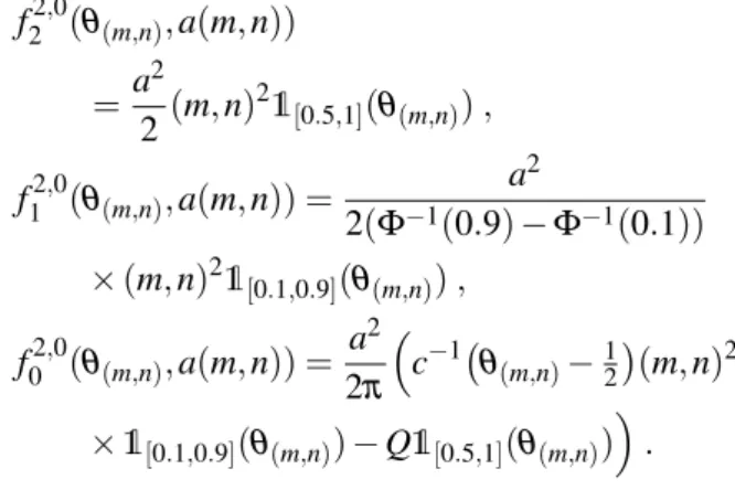
do not depend on surface normals, only 1×1 configurations are necessary in the estimators. The respective (tensor-valued) weight functions are

f₂2,0(θ(m,n),a(m,n))

=a

2

2 (m,n)

2₁

[0.5,1](θ(m,n)),

f₁2,0(θ(m,n),a(m,n)) =

a2

2(Φ−1(0.9)−Φ−1(0.1))

×(m,n)21[0.1,0.9](θ(m,n)),

f₀2,0(θ(m,n),a(m,n)) = a2 2π

c−1 θ(m,n)−1₂

(m,n)2

×1[0.1,0.9](θ(m,n))−Q1[0.5,1](θ(m,n))

.

Here the constantcis given by

c=2!

Z −Φ−1(0.1)

Φ−1(0.1)

tΦ(−t)dt≈ −0.961.

The reason for this scaling is that for our PSF, the constantc=2(c1+c2+c3) in the notation of Svane

(2014b). The tensor(m,n)2_{may also be interpreted as}

the 2×2 matrix(m,n)T(m,n).

The estimator is again given by summing these weights over all lattice points:

ˆ

Φ2_k,0(X) =ak

_∑

a(m,n)∈a_Z2

f_k2,0(θ₍m,n),a(m,n)).

Note that while the estimators withk=1,2 converge to the true value, Corollary 16 does not show convergence for k=0, since the Gaussian does not have compact support.

DISCUSSION

The paper shows that, contrary to black-and-white images, there is information enough in digital grey-scale images to extract some of the surface and mean curvature tensors based only on local information. This extends the known results for Minkowski functionals from Svane (2014b). The new finding is that position dependent surface integrals can also be estimated by allowing the weight function to depend on position. Moreover, by considering 2× · · · ×2 configurations, it is possible to locally determine directions of surface normals.

However, the new estimators are no longer simple. While the estimators for surface area could be based on an image thresholded at two different levels, detailed information about the PSF is needed for the surface tensors.

or not this is realistic will depend on the way the blurring arises, see the discussion in Svane (2014b). For intrinsic volumes, only the convergence of the PSF was essential, but when taking larger configurations into account, an assumption on the convergence of resolution is necessary.

It still remains to investigate how the algorithms work out in finite resolution. For this, simulation studies could provide an idea about their performance. To apply the algorithms in practice would require a set-up that matches the assumptions. In particular, one needs to know the PSF or at least what a blurred halfspace looks like. The latter might be tested experimentally or by fitting a PSF. Moreover, the PSF has to be rotation invariant and the resolution needs to be high compared to the blurring,cf.Condition (iii).

It is still unknown whether the lower Minkowski tensors can be estimated in a similar way - even in the basic case of Minkowski functionals.

ACKNOWLEDGEMENTS

The author was funded by a grant from the Carlsberg Foundation and hosted by the Institute of Stochastics at Karlsruhe Institute of Technology. The author would also like to thank Markus Kiderlen for helpful input and suggestions.

REFERENCES

Airy GB (1835). On the diffraction of an object-glass with circular aperture. Trans Cambridge Philos Soc 5:283– 91.

Federer H (1959). Curvature measures. Trans Amer Math Soc 93:418–91.

Hug D, Last G, Weil W (2004). A local Steiner-type formula for general closed sets and applications. Math Z 246:237–72.

Hug D, Schneider R, Schuster R (2008). Integral geometry of tensor valuations. Adv Appl Math 41:482-509. Kampf J (2012). A limitation of the estimation of intrinsic

volumes via pixel configuration counts. WiMa Report 144.

Kiderlen M, Rataj J (2007). On infinitesimal increase of volumes of morphological transforms. Mathematika 53:103–27.

Klette R, Rosenfeld A (2004). Digital geometry. San Francisco: Elsevier.

K¨othe U (2008). What can we learn from discrete images about the continuous world? In: Coeurjolly D, Sivignon I, Tougne L, Dupont F, eds. Discrete Geometry for Computer Imagery, Proc DGCI 2008. Berlin: Springer. Lect Not Comput Sci 4992:4–19.

Matheron G (1975). Random sets and integral geometry. Toronto: John Wiley & sons.

McMullen P (1997). Isometry covariant valuations on convex bodies. Rend Circ Mat Palermo (2), Suppl. 50:259–71.

Ohser J, M¨ucklich, F (2000). Statistical analysis of microstructures. Chichester: John Wiley & Sons. Schneider R (1993). Convex bodies: The Brunn–Minkowski

theory. Cambridge: Cambridge University Press. Schneider R, Schuster R (2002). Tensor valuations on

convex bodies and integral geometry, II. Rend Circ Mat Palermo (2), Suppl 70: 295314.

Schr¨oder-Turk GE, Kapfer SC, Breidenbach B, Beisbart C, Mecke K (2008). Tensorial Minkowski functionals and anisotropy measures for planar patterns. J Microsc 238:57–74.

Schr¨oder-Turk GE, Mickel W, Kapfer SC, Schaller FM, Breidenbach B, Hug D et al. (2010a). Minkowski tensors of anisotropic spatial structure. New J Phys 15:083028.

Schr¨oder-Turk GE, Mickel W, Schr¨oter M, Delaney GW, Saadatfar M, Senden TJ et al. (2010b). Disordered spherical bead packs are anisotropic. Europhys Lett 90:34001.

Schr¨oder-Turk GE, Mickel W, Kapfer SC, Klatt MA, Schaller FM, Hoffmann MJ et al. (2011). Minkowski tensor shape analysis of cellular, granular and porous structures. Adv Mater 23:2535–53.

Svane AM (2014a). On multigrid convergence of local algorithms for intrinsic volumes. J Math Imaging Vis 49:352–76.