City, University of London Institutional Repository
Citation
: Pesenti, S. M., Millossovich, P. ORCID: 0000-0001-8269-7507 and Tsanakas, A.
ORCID: 0000-0003-4552-5532 Cascade Sensitivity Measures. .
This is the preprint version of the paper.
This version of the publication may differ from the final published
version.
Permanent repository link:
http://openaccess.city.ac.uk/id/eprint/20808/Link to published version
:
Copyright and reuse:
City Research Online aims to make research
outputs of City, University of London available to a wider audience.
Copyright and Moral Rights remain with the author(s) and/or copyright
holders. URLs from City Research Online may be freely distributed and
linked to.
City Research Online: http://openaccess.city.ac.uk/ [email protected]
Cascade Sensitivity Measures
∗
Silvana M. Pesenti†1, Pietro Millossovich2,3, and Andreas Tsanakas2
1Department of Statistical Sciences, University of Toronto
2Cass Business School, City, University of London
3DEAMS, University of Trieste
23. July 2019
Abstract
In risk analysis, sensitivity measures quantify the extent to which the probability
distri-bution of a model output is affected by changes (stresses) in individual random input factors.
For input factors that are statistically dependent, we argue that a stress on one input should
also precipitate stresses in other input factors. We introduce a novel sensitivity measure,
termedcascade sensitivity, defined as a derivative of a risk measure applied on the output,
in the direction of an input factor. The derivative is taken after suitably transforming the
random vector of inputs, thus enabling the cascade sensitivity measure to capture both the
direct impact of the stressed input factor on the output, as well as indirect effects via other
input factors that are dependent on the one being stressed. Alternative representations of
the cascade sensitivity measure, which can be calculated from a single Monte Carlo sample,
are provided for two types of stress: a) a perturbation of the distribution of an input
fac-tor such that the stressed input follows a mixture distribution, and b) an additive random
shock applied to the input factor. The calculation of those representations does not require
simulating under different model specifications or the explicit study of the properties of
the model function, making the proposed method attractive for applications, as illustrated
through numerical examples.
∗
Earlier versions have been presented at the University of Trieste, at the University of Milano-Bicocca, at
the10thConference in Actuarial Science & Finance (Samos), at the4th European Actuarial Journal Conference
(Leuven), at theWorkshop on Recent Developments in Dependence Modelling with Applications in Finance and
Insurance (Aegina), at the KU Leuven & Cass Business School PhD colloquium (Leuven), at the University
of Liverpool, at the RiskLab, ETH Zurich, at the Vrije Universiteit Brussel and at the Ninth International
Conference on Sensitivity Analysis of Model Output (Barcelona). The authors are grateful for discussions with
and comments from Vali Asimit, Patrick Cheridito, Paul Embrechts, Mike Ludkovski, Ludger R¨uschendorf, Steven
Vanduffel, Ruodu Wang and Mario W¨uthrich.
†
Keywords Sensitivity analysis, importance measures, perturbation analysis, risk measures,
importance sampling, dependence, Rosenblatt transform.
1
Introduction
1.1 Overview and contribution
Sensitivity analysis is concerned with the attribution of the uncertainty of a model output to
the uncertainties of a model input (Saltelli et al.,2008). Principal tools in sensitivity analysis
are sensitivity measures (also called ‘importance measures’), which assign to each input factor
a score, ranking inputs according to their ability to influence (a probabilistic summary of) the
output, seeBorgonovo and Plischke (2016) for an extensive review. Variance-based sensitivity
measures, for example, distinguish input factors by their ability to affect the output’s variance
(Saltelli, 2002). In this paper, and as is typical in risk management applications, the output
distribution is summarized through a quantile-based measure of risk. Specifically, we consider
the class of distortion risk measures introduced by Wang (1996), which subsumes expected
utilities and the two most common risk measures in financial risk management, Value-at-Risk
(VaR) and Expected Shortfall (ES).
Sensitivity measures are often constructed via partial derivatives either of outputs with
re-spect to inputs (‘local’ sensitivity measures, see Borgonovo and Plischke (2016) and references
therein) or of the output risk measure in the direction of random inputs (Tsanakas and
Mil-lossovich, 2016;Antoniano-Villalobos et al.,2018). One drawback of such sensitivity measures
is that they do not fully account for interactions among or statistical dependence between input
factors. Extensions have so far focused on higher order derivatives (Mara and Tarantola,2012;
Borgonovo and Plischke, 2016). However, dependence structures between input factors might
substantially impact the sensitivity to an input factor, as is illustrated in the following example.
Example (Non-linear insurance portfolio). Consider an insurance company with losses from
three different lines of business,X1, X2andX3, each of which is subject to the same
multiplica-tive factorX4 arising from, e.g. inflation. The insurance company holds a reinsurance contract
on the loss from the first two lines of business, L=X4(X1+X2), with deductible dand limit
l. This means that the aggregate loss faced by the insurer is
Y =L−min{(L−d)+, l}+X3X4. (1)
In this simple model, which we will use as a running example throughout the paper, we view
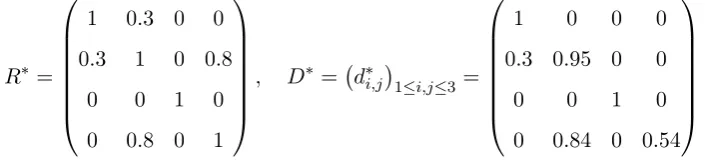
(X1, X2, X3, X4) are dependent through a Gaussian copula with correlation matrixR:
R =
1 0.3 0 0.8
0.3 1 0 0
0 0 1 0
0.8 0 0 1
.
Each elementrij ofR closely approximates the Spearman rank correlation CorrS(Xi, Xj) of the
respective pair of input factors. Note that the aggregate portfolio lossY is symmetric inX1 and
X2but the dependence structure is not;X1 has a high rank correlation toX4, CorrS(X1, X4) =
0.8, while CorrS(X2, X4) = 0. Measuring the sensitivity to X1 and X2, via a local method
involving ∂X∂Y
1,
∂Y
∂X2, obviously fails to reflect the asymmetry in statistical dependence. More
generally, as is demonstrated in the continuation of this example in Section3, such asymmetry
is also not fully reflected by global sensitivity measures based on partial derivatives, in the vein
of Tsanakas and Millossovich(2016).
Example (London Insurance Market portfolio). Consider the situation of a model user or
re-viewer, who has only partial access to the model specifications. It is typical in risk management
applications, for models to be high dimensional with calculation of the model’s output
distri-bution proceeding by Monte Carlo simulation (Arbenz et al.,2012;Choe et al.,2018;Risk and
Ludkovski,2018). A model user will often be supplied with a set of simulated scenarios from
variables of interest (model inputs or outputs), without easy access to either (a) the
distribu-tional assumptions of inputs (which may themselves be outputs from sub-models) or (b) the
model function mapping inputs to outputs (which may be highly non-linear and
computation-ally expensive to evaluate). This situation is typical in the regulatory review of internal models
in insurance (Cadoni,2014).
For illustration of those points, we consider a proprietary model of a London Insurance
Market portfolio, currently in use by a participant in that market. The model represents
a portfolio with 72 input factors; the output is the portfolio loss. We do not have access
to the marginal nor the joint distribution of the input vector; indeed, the input factors are
themselves outputs of different models. We were supplied by the model owner with a Monte
Carlo sample of size M = 500,000, consisting of simulated observations from the model’s
inputs and corresponding output. We have no access to the data generating mechanism, hence
we cannot re-simulate under different model assumptions.
In Figure 1we summarize the distributions of individual input risk factors, by plotting the
mean and the Expected Shortfall risk measure (at 90% level) of each. The question we aim to
0.5
1.0
1.5
2.0
2.5
Input risk factor
Mean and ES (p=0.9) of r
isk f
actors
● ●
● ● ● ● ● ● ●● ● ● ● ●
● ● ● ● ● ● ● ● ● ● ● ● ● ●
● ● ● ● ● ● ● ● ● ● ● ● ● ● ● ● ● ● ● ● ● ●● ● ● ● ● ● ● ●
● ● ● ● ● ● ● ● ● ●
● ● ●
●
41 9
45543522 5 4851282952473716
30363313325631716558691134596821635561462326622070 6 49 4 12 2 3 1 5060 7 3814
1939572527536440181567104344 8 42
246672 17
[image:5.595.92.475.127.318.2]● mean ES
Figure 1: Expected value and ES0.9 risk measure of input risk factors in the London Market
portfolio.
of perturbations in a particular risk factor, taking fully into account the dependence between
inputs? We return to this example in Section 5.
In this paper, we aim to address the issues raised by the preceding two examples. We propose
a novel sensitivity measure, termed cascade sensitivity, which explicitly accounts for the direct
and indirect dependence between input factors. Specifically, the cascade sensitivity is defined
as the partial derivative of a distortion risk measure applied to the output, in the direction of
a stressed input factor; hence it is closely related to the approaches of Hong (2009);Hong and
Liu(2009);Tsanakas and Millossovich(2016). However, in our case the derivative is taken after
a suitable transformation of the random vector of inputs, which enables cascade sensitivity
measures to fully capture the impact of dependence between input factors. Specifically, our
cascade sensitivity framework is underpinned by a variation of the inverse Rosenblatt transform
(Rosenblatt,1952), which permits a stress on one input factor to propagate through the entire
input vector, changing all its components according to the input vector’s dependence structure.
Thus, a stress on an input impacts on the output risk measure both directly and indirectly,
via the generated cascade of stresses on other (dependent) inputs. In particular, the cascade
contribution of an input factor to the sensitivity of the output.
A sensitivity measure that fully reflects the dependence of the random vector of inputs is
useful in applications where the dependence structure of the inputs is of particular interest, as in
risk management applications (Glasserman and Xu,2014;Lam,2017). The computational costs
of evaluating importance measures is a persistent theme in the sensitivity analysis literature
(Saltelli et al., 2008;Lam and Qian, 2018), given the need for costly evaluations of the (high
dimensional, non-linear) model function at different simulated scenarios. We provide explicit
analytical representations of the cascade sensitivity, which do not require calculation of the
gradient of the aggregation function and allow for a straightforward implementation on a single
Monte Carlo sample, thus avoiding multiple model runs. These alternative representations of
the cascade sensitivity are derived for two types of stress on an input factor: a) a perturbation
of the distribution of an input factor, such that the stressed input factor follows a mixture
distribution, and b) an additive random shock applied to the (tail of the) input factor itself.
Hence, our proposed cascade sensitivity framework is practically useful, as illustrated through
an application to a commercially used London Insurance Market portfolio model.
1.2 Relation to existing literature
The statistical functional whose sensitivity we are evaluating, i.e. a composition of a risk
measure with a multivariate (non-linear) aggregation function, also appears in the study of
systemic risk (Chen et al.,2013). While we do not actively purse this interpretation, systemic
risk quantification is within the scope of the methods developed in the present paper.
Derivatives of distortion risk measures, applied to a model output in the direction of an
input, have been extensively studied in sensitivity analysis and in capital allocation; notably by
Hong(2009);Cont et al. (2010) for the VaR risk measure,Hong and Liu(2009) for the ES risk
measure andTsanakas and Millossovich(2016) for general distortion risk measures. Sensitivity
to linear portfolios summarized by Haezendonck-Goovaerts and entropic risk measures are
con-sidered in Wang et al. (2018) and Tsanakas (2009), respectively. Cao and Wan(2017) analyse
derivatives of expected utilities in connection to optimal portfolio selection, while Gourieroux
et al. (2000, 2006) consider directional derivatives of distortion risk measures with respect to
parameter uncertainty for linear aggregation functions. See also Antoniano-Villalobos et al.
(2018) for a discussion on sensitivity measures to input parameters. However, in this stream of
literature, sensitivity measures generally do not account explicitly for the impact of the
depen-dence between input factors and thus do not lend themselves to investigations of dependepen-dence
Uncertainty in the dependence of an input vector is typically addressed by calculating the
worst-case of a risk measure applied on the output, such that the input vector belongs to an
uncertainty set. We refer toGlasserman and Xu(2014);Lam(2016,2017);Pesenti et al.(2019)
for uncertainty sets defined though probability distances and toEmbrechts et al.(2013);Wang
and Wang(2016);Li(2018) for worst-case spectral risk measures. While these papers deal with
dependence uncertainty, by assessing risk on (potentially unrealistic) worst-case models, they
not fully address the sensitivity to dependence of the baseline models in use.
The Rosenblatt transform has been used in various statistical contexts, e.g. see Dawid
(1984), but only recently has it been utilized to measure effects of dependence between input
factors for sensitivity purposes. Notable contributions are Mai et al. (2015), who study model
robustness through introducing uncertainty via a transformation of the input vector, andMara
and Tarantola (2012) in the context of variance based sensitivity measures. Kraus and Czado
(2017) carry out bank stress testing using graphical (D-vine) dependence models; their approach,
while methodologically different, is conceptually close to the ideas in this paper.
Further work related to ours is the stream of research on quantile sensitivity estimation in a
Monte Carlo simulation setting. Sensitivity to quantiles, as well as risk contributions, typically
involves estimation of conditional expectations, where the conditioning event has small or zero
probability of occurring. State-of-the-art estimators rely on variance reduction techniques such
as importance sampling, see Fu et al. (2009); Glasserman and Li (2005); Tasche (2009) and
Merino and Nyfeler (2004) for an application of importance sampling to risk contributions of
VaR and ES, respectively. Restricted importance sampling, a variation of importance sampling,
has recently been proposed by Liu (2015) to improve convergence rates of estimators of risk
contributions.
1.3 Structure of the paper
The paper is organized as follows. Section 2 introduces the notation and mathematical
frame-work. In section3the cascade sensitivity measure is defined as a partial derivative of a distortion
risk measure applied to the output, in the direction of a stressed input factor, via a variation
of the inverse Rosenblatt transform. The impact of input vectors’ dependence structure on
sensitivity is discussed and illustrated through numerical examples.
Section 4 is devoted to the calculation of the cascade sensitivity. We provide alternative
representations of the cascade sensitivity for two classes of stresses that allow for calculations
on a single Monte Carlo sample by importance sampling. The applicability of the cascade
We conclude in Section 5, with an application of cascade sensitivity to the commercially used
London Insurance Market portfolio discussed above, illustrating the challenges of sensitivity
testing ‘black box models’. All technical assumptions, proofs and detailed analytical calculations
for the examples are gathered in Appendix A.
2
Preliminaries
Throughout the paper we work with a probability space (Ω,A, P) and a random vector X = (X1, . . . , Xn) whose integrable components, X1, . . . , Xn, represent input factors. We denote
by Fj the marginal distribution function of the input Xj, j = 1, . . . , n, and by F the joint
distribution function of X. It is assumed that the joint density f of X exists and we denote by fj the marginal density of input factor Xj, j= 1, . . . , n. The vector of input factors, X, is
mapped by anaggregation function,g:Rn→R, assumed to be almost everywhere differentiable,
to the (univariate) outputY =g(X). We writeH, hfor the distribution function and the density of the outputY, respectively.
The left inverse of the distribution of any random variableW ∼FW is defined byFW−1(u) =
inf{x ∈R | FW(x) ≥u}, u∈(0,1]. We use the notation UW for a standard uniform random
variable comonotonic toW, that is, W =FW−1(UW) a.s. In the case when W has a continuous
distribution function, it holds thatUW =FW(W). Moreover, for an n-dimensional vector W,
we denote byW−j = (W1, . . . , Wj−1, Wj+1, . . . Wn) its sub-vector deprived of thejthcomponent.
The distribution of the output Y =g(X)∼H, representing a decision variable, is summa-rized through a risk measure. Risk measures are tools in financial risk management to assess
different levels of risk severity (Artzner et al.,1999; F¨ollmer and Schied,2011). Here we work
with the class ofdistortion risk measuresintroduced byWang(1996);Acerbi and Tasche(2002),
which are defined through
ργ(Y) = Z 1
0
H−1(u)γ(u)du=E H−1(UY)γ(UY)
,
where γ: [0,1]→ [0,∞) is a normalized weight function such that R1
0 γ(u)du = 1. The focus
on distortion risk measures is not restrictive, as the proposed framework is also applicable for
utility type performance measures, see the remark at the end of Section 3.1. Throughout this
paper, the examples will be based on the two most common distortion risk measures used in
practice, VaR and ES. The VaR of the random variable Y at level α ∈ (0,1) is defined as its
the left α-quantile, VaRα(Y) = H−1(α) or through the weight function γ(u) =δα(u), for the
Dirac measureδα. The ES, also called Conditional Value-at-Risk, at levelα∈[0,1) arises from
γ(u) = 1−α1 1{u>α}, thus has representation ESα(Y) = 1−α1 R1
αH
The objective of this paper lies in the study of the sensitivity of ργ(Y) to input factor
Xi, 1 ≤ i ≤ n. For simplicity, we fix i ∈ {1, . . . , n} for the rest of the paper, such that
sensitivity to the same input is considered throughout. We call a stress on input factor Xi a
family of random variables Xi,ε(ω) = K(Xi(ω), ω, ε), for ε≥ 0,ω ∈Ω and some mapping K,
that is almost everywhere differentiable in ε in a neighbourhood of 0, uniformly in x and ω.
Moreover, K satisfies K(x, ω,0) = x, for all x ∈ R and almost all ω ∈ Ω. In particular, for
any stressXi,ε, it holds that (X1, . . . , Xi,ε, . . . , Xn)|ε=0 =X a.s. We denote byFi,ε, ε≥0, the
distribution function of Xi,ε.
A typical choice of a stress is to apply a random shock Z to the input factorXi, such that
Xi,ε= Xi+εZ (Tsanakas and Millossovich, 2016). Alternatively, the distribution function of
the input factor,Fi, can be perturbed, an approach conceptually different from adding a shock.
Adding uncertainty via the distribution function of the input factor is a common technique
in sensitivity analysis and also used in Bayesian and robust statistics (Hampel et al., 2011;
Borgonovo and Plischke,2016;Glasserman,1991;Saltelli et al.,2008). Such aperturbation can
be constructed starting from a family of distribution functions Fi,ε,ε≥0, that is continuously
differentiable in ε, admits a density for all ε in a neighbourhood of 0, and fulfills Fi,0 = Fi.
We then define the stress to input factor Xi through a perturbation by Xi,ε =Fi,ε−1(Z), for a
standard uniform random variable Z. Depending on the choice of Z, the stress may not only
distort the input factorXi but might also change the dependence structure of the input vector
X. A natural choice, which we consider in the sequel, isZ to be comonotonic toXi, generating
perturbations of the form Xi,ε = Fi,ε−1(UXi), thus not altering the dependence between input
factors.
3
Sensitivity measures
3.1 Marginal sensitivity
To assess the sensitivity of the outputY to the inputXi, sensitivity measures are defined. The
approach we follow here is to take a directional derivative of the risk measure applied to the
output distribution, in the direction of a stress to input Xi.
Definition 3.1. For a stress Xi,ε and a distortion risk measure ργ, we define the marginal
sensitivity to input factor Xi by
Si(X, g, ργ) =
∂
∂εργ g(X1, . . . , Xi,ε, . . . , Xn)
ε=0,
The general form of the marginal sensitivity for distortion risk measures follows directly
from Hong and Liu (2009) and stated in the next proposition for completeness. It consists of
an expectation involving the derivative of the stress, the partial derivative of the aggregation
function in the direction of the stressed input factor and a weighting according to the chosen
risk measure.
Proposition 3.2. Given a stressXi,εand under AssumptionsA.1in the appendix, the marginal
sensitivity to input factorXi is
Si(X, g, ργ) =E ∂
∂εXi,ε
ε=0gi(X)γ(UY)
,
where gi(x) = ∂x∂ig(x) denotes the partial derivative of the aggregation function in the ith
component and ∂ε∂Xi,ε(ω) = ∂ε∂K(Xi(ω), ω, ε), for almost allω∈Ω.
Remark. Further work on derivatives of risk measures, and closely related to ours, is Hong
(2009);Tsanakas and Millossovich (2016). Our framework also includes sensitivity of expected
utilities, considered in Cao and Wan (2017); Antoniano-Villalobos et al. (2018). Note that,
for the trivial weight function γ ≡ 1, the distortion risk measure reduces to the expectation,
ρ1(·)≡E(·). Thus, for an utility functionu:R→R, we can write
E(u(g(X)) =ρ1 (u◦g)(X)
,
implying that expected utilities are a special case of our framework, with aggregation function
u◦g:Rn→Rand an expectation risk measure.
3.2 Inverse Rosenblatt transforms
The marginal sensitivity of Definition 3.1 does not fully account for interactions among or
dependence between input factors, since, by its definition, when stressing one input factor, all
other marginal input distributions remain unaltered; see also the discussion in Borgonovo and
Plischke (2016). Note that the representation of the marginal sensitivity in Proposition 3.2
incorporates the derivative of the aggregation function solely in the direction of the stressed
input factor.
In order to address the indirect effects induced by the dependence between the input factors,
we utilize a representation of random vectors, termedinverse Rosenblatt transform (Rosenblatt,
1952;R¨uschendorf and de Valk,1993).1
1
We call representation (2) theinverse Rosenblatttransform since, to be precise, the Rosenblatt transform is
Definition 3.3. An inverse Rosenblatt transform of ann-dimensional random vectorX, start-ing at Xi, is given by a differentiable function ψ = (ψ(1), . . . , ψ(n))>:Rn →Rn and a (n− 1)-dimensional random vector V = (V1, . . . , Vn−1), consisting of independent standard uniform
variables, independent of Xi, such that
X =ψ(Xi,V) = ψ(1)(Xi,V), . . . , ψ(n)(Xi,V)
a.s. (2)
The set of inverse Rosenblatt transforms ofX, starting atXi, is denoted byRi ={(ψ,V)|X =
ψ(Xi,V)}.
It can be shown that forψ(j), 1≤j≤n, to exist and be differentiable in the first component,
it is sufficient that the joint density f is almost everywhere differentiable.
An inverse Rosenblatt transform can be explicitly constructed via the following process
(R¨uschendorf and de Valk, 1993; Rubinstein and Melamed, 1998). For r = 1, . . . , n and J ⊆
{1, . . . , n}\{r}, denote by Fr|J(· | xj, j ∈J) the conditional distribution function ofXr given
Xj =xj, j ∈J. Then, it holds a.s. that
X1=F1−|i1(V1|Xi) =ψ(1)(Xi,V),
X2=F2−|i,11(V2|Xi, X1) =ψ (2)(X
i,V),
X3=F3−|i,11,2(V3|Xi, X1, X2) =ψ (3)(X
i,V),
.. .
Xi=ψ(i)(Xi,V),
.. .
Xn=Fn|−11,...,n−1(Vn−1|X1, . . . Xn−1) =ψ(n)(Xi,V),
where ψ(i) is the identity function in the first argument. Note that in the above construction,
each random variableXj depends onXi both directly and indirectly throughX1, . . . , Xj−1.
Deploying an inverse Rosenblatt transform of the vector X =ψ(Xi,V), (ψ,V) ∈ Ri, we
can stress input Xi throughXi,ε
Xi,ε=ψ(Xi,ε,V) = ψ(1)(X1,ε,V), . . . , ψ(n)(X1,ε,V)
. (3)
Observe that the stress Xi,ε is carried through the entire input vector, changing all factors
according to their dependence onXi,ε, resulting in a cascading effect.
this example, thati= 1. For a vector of independent standard uniformsV = (Vj)j=1,...,n−1
inde-pendent ofX1, define the standard normal variablesZ1= Φ−1 F1(X1)
andTj = Φ−1(Vj), j=
1, . . . , n−1. Then, an inverse Rosenblatt transform starting fromX1, (ψ,V) ∈ R1, is derived
by setting
ψ(1)(X1,V) =X1
ψ(2)(X1,V) =F2−1 Φ (d21Z1+d22T1)
.. .
ψ(n)(X1,V) =Fn−1 Φ (dn1Z1+dn2T1+· · ·+dnnTn−1)
,
where Φ denotes the standard normal distribution function and D = (di,j)1≤i,j≤n is the lower
triangular matrix resulting from the Cholesky decomposition of R. Following this
represen-tation, one can stress X1 through substitution by X1,ε, which implies substituting Z1 by
Z1,ε = Φ−1 F1(X1,ε)
, in the right hand-side of the above equations. It is then apparent
how the stress on X1 also produces a stress on Xj, j = 2, . . . , n (provided dj1 6= 0).
3.3 Cascade sensitivity
The inverse Rosenblatt transform, by propagating stresses on one input factor across the vector
of inputs, allows us to construct a sensitivity measure that fully reflects both the direct and
indirect the impacts on the output.
Definition 3.4. For a stress Xi,ε, (ψ,V)∈ Ri and a distortion risk measure ργ, we define the
cascade sensitivity to input factorXi by
Ci(X, g, ργ) =
∂
∂εργ g ψ(Xi,ε,V)
ε=0,
whenever the derivative exists.
Hence, the cascade sensitivity framework directly extends approaches to sensitivity analysis
that are based on partial derivatives in the direction of input factors, to fully account for
dependence of input factors. In particular, the cascade and the marginal sensitivities only
differ in the way a stress on an input propagates across the whole vector of input factors, there
being no account for propagation in the marginal case. Though the current paper is focused on
distortion risk measures (and expected utilities), the use of the inverse Rosenblatt transform for
sensitivity analysis is a tool that could also be used in other (e.g. variance-based) sensitivity
The cascade sensitivity to an input factor can be decomposed into the marginal sensitivity
and additional components, each reflecting statistical, as well as functional, dependence between
inputs.
Proposition 3.5. Given a stress Xi,ε, (ψ,V) ∈ Ri, and under Assumptions A.1 in the
ap-pendix, the cascade sensitivity to input factorXi is
Ci(X, g, ργ) = n X
j=1
Ci,j, (4)
where
Ci,j =E ∂
∂εXi,ε
ε=0gj(X)ψ (j)
1 (Xi,V)γ(UY)
,
forj= 1, . . . , n.
The set of inverse Rosenblatt transforms of a random vector,Ri, is generally not a singleton,
implying that the inverse Rosenblatt transform is not unique. For instance, in the last example,
a different tranform would be obtained for some permutation of (X2, . . . , Xn). However, as the
next result shows, the cascade sensitivity does not depend on the particular choice of inverse
Rosenblatt transform, (ψ,V)∈ Ri.
Proposition 3.6. If the cascade sensitivity exists for one (ψ,V) ∈ Ri, then it exists and admits the same value for all other transforms (φ,U) ∈ Ri. Moreover, decomposition (4) is
unique.
The decomposition of the cascade sensitivity Ci in Proposition 3.5 allows to quantify the
contribution of each input factors’ indirect effects, stemming from the dependence with the
one being stressed, to Ci. Specifically, Ci,j is the indirect contribution of input Xj to the
sensitivity Ci, when stressing input factor Xi. Moreover, note that Ci,i = Si is the marginal
sensitivity; hence Ci − Ci,i is the component of the cascade sensitivity which is solely due to
the dependence structure between input factors. The components Ci,1, . . . ,Ci,n, contributing to
the cascade sensitivities, Ci, i = 1, . . . , n, can be visualized as shown below. Each row shows
a cascade sensitivity decomposed into its n-summands, Ci = Pnj=1Ci,j, i = 1, . . . , n. The
diagonal contains the marginal sensitivities, while off-diagonal elements Ci,j reflect the indirect
contribution of Xj to the cascade sensitivity of Xi.
Remark. The cascade sensitivity framework also includes sensitivity to uncertain statistical
parameters of input factors (Antoniano-Villalobos et al.,2018). Let Fi|Θi(·|θi) denote the
con-ditional distribution of Xi given parameter Θi=θi. Then it holds almost surely that
X1 X2 . . . Xn
C1 S1 C1,2 . . . C1,n
C2 C2,1 S2 . . . C2,n
..
. ... ... . .. ...
Cn Cn,1 Cn,2 . . . Sn
for a function η: R2 → R and a standard uniform random variable Ui independent of Θi.
Hence, instead of stressing the input factor Xi, we can perturb the variables Θi and Ui via
representation (5), in this way reflecting the sensitivity ofργ(Y) to the parameter and process
uncertainty ofXi, respectively.
Example (Non-linear insurance portfolio continued). We calculate the cascade sensitivity for
the insurance portfolio example introduced in Section1, assuming that the two lines of business,
X1, X2, are each modelled by a Log-Normal(µ= 4.98, σ2= 0.232) distribution with mean 150
and standard deviation 35. The third line of business,X3, follows a Gamma(100,1) distribution
with mean 100 and standard deviation 10, while the multiplicative factor,X4, is assumed to be
Log-Normal(µ4 =−0.005, σ24 = 0.12) distributed, that is with mean 1 and standard deviation
0.1. All the calculations are based on a simulated Monte Carlo sample of sizeM = 100,000.
We consider an additive shock to the first two lines of business defined byXi,ε=Xi+ε(Xi−
m), i= 1,2, wherem= 138.5 is the mode of either. Stressing relative to the mode is motivated
by Section4.2, as it results in an easily tractable calculation of the cascade sensitivity on a single
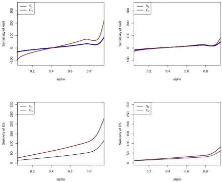
Monte Carlo sample. Figure2displays the marginal and cascade sensitivity to input factorsX1
and X2 for the risk measure VaRα (top) and for ESα (bottom), for 0.075< α <0.925. Note
that the marginal and the cascade sensitivity for the second line of business,X2, are fairly close
(compared to the sensitivities toX1), indicating that the indirect effects contributing toC2 are
minor (compared to those of C1).
The choice of distortion risk measure has a notable impact on the sensitivities, as seen by
comparing the top (VaR) and the bottom (ES) plots. This is particularly pronounced when
contrasting the marginal and the cascade sensitivity toX1. While the VaR is defined through the
Dirac weight function, hence only encompasses a single point, γ(·) =δα(·), the weight function
of the ES, γ(·) = 1−α1 1{·>α}, incorporates the entire right tail of the output’s distribution function. Thus, sensitivities utilising VaR can be seen as local measures of sensitivity, since
inputs are assessed in how they affect one quantile of the output’s distribution function. This
is in contrast to employing the ES, which leads to a ranking of inputs according to their ability
0.2 0.4 0.6 0.8
−100
0
100
200
300
alpha
Sensitivity of V
aR
S1
C1
0.2 0.4 0.6 0.8
−100
0
100
200
300
alpha
Sensitivity of V
aR
S2
C2
0.2 0.4 0.6 0.8
0
50
100
150
200
250
300
alpha
Sensivity of ES
S1
C1
0.2 0.4 0.6 0.8
0
50
100
150
200
250
300
alpha
Sensivity of ES
S2
[image:15.595.70.511.100.461.2]C2
Figure 2: Marginal and cascade sensitivity to input factorX1 (left) and input factorX2 (right),
for stresses Xi,ε=Xi+ε(Xi−m), where m is the mode ofXi, i= 1,2. The top displays the
sensitivities for the risk measure VaRα and the bottom graphs depict the risk measure ESα, for
0.075< α <0.925.
sensitivities to X1 and to X2, as functions of α, cross once, that is, S1 ≤ S2, C1 ≤ C2 for α
small and S1 ≥ S2, C1 ≥ C2 forα close to 1, whereas for ESα the sensitivities to X2 dominate
the corresponding sensitivities toX1, that is C2≥ C1 andS2 ≥ S1 for all 0≤α <1.
Table1reports the cascade sensitivities to inputs X1 andX2 for the risk measure ES0.9. In
this particular example, the terms reflecting the indirect effects of the dependence between the
input factors are scaled according to their Spearman rank correlation with the stressed input
factor, that is, Ci,j is proportional to CorrS(Xi, Xj) (for explicit calculations see A.3). Note
that CorrS(X2, X3) = CorrS(X2, X4) = 0, hence C2,3 =C2,4 = 0, and thus C2 =C2,1+S2 only
Table 1: The cascade sensitivities to inputs X1, X2 (along with standard errors) for ES0.9 and
its decomposition into the direct effect of the stressed input (Ci,i =Si) and the indirect effects
of the other input factors (Ci,j).
Ci,1 Ci,2 Ci,3 Ci,4
C1= 162.93 (0.017) 79.61 (0.009) 19.28 (0.002) 0 64.04 (0.006)
C2= 59.14 (0.009) 13.68 (0.002) 45.47 (0.007) 0 0
indirect impact of X4,C1,4, constitutes a substantial 39% = 16264..0493 to the cascade sensitivity to
X1.
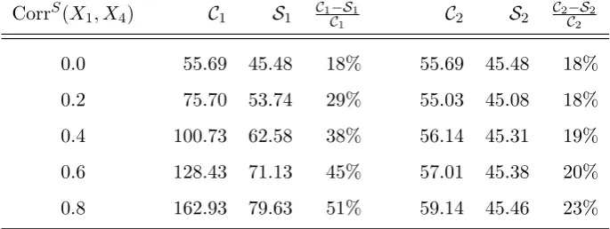
To further illustrate the effects of the dependence structure of the input vector on cascade
sensitivities, we report the marginal and cascade sensitivities for ES0.9, with CorrS(X1, X4) =
0.0, . . . ,0.8 in Table 2. Table2 also states the percentage of the cascade sensitivity that stems
solely from the effects of the dependence between inputs, Cj−Sj
Cj , j = 1,2. As seen in Table
2, both the marginal and the cascade sensitivity to X1 increase with CorrS(X1, X4), with C1
impacted more heavily. The marginal sensitivity to input X2 is practically constant, implying
that changes in the dependence between X1 and X4 only have a very minor impact on S2,
which is in contrast to the cascade sensitivity to inputX2, which increases by 6.2% = (59.14−
[image:16.595.126.469.497.626.2]55.69)/55.69, thus reflecting such indirect effects.
Table 2: Marginal and cascade sensitivity for the ES0.9 with CorrS(X1, X4) = 0.0, ...,0.8.
CorrS(X1, X4) C1 S1 C1C−S1 1 C2 S2 C2C−S2 2
0.0 55.69 45.48 18% 55.69 45.48 18%
0.2 75.70 53.74 29% 55.03 45.08 18%
0.4 100.73 62.58 38% 56.14 45.31 19%
0.6 128.43 71.13 45% 57.01 45.38 20%
0.8 162.93 79.63 51% 59.14 45.46 23%
3.4 Comparison of the marginal and cascade sensitivities
Proposition 3.5 showed that the cascade sensitivity decomposes into the marginal sensitivity
and components reflecting the dependence between the input factors. Thus, a natural question
arises to whether, in general, positive (negative) dependence among inputs results into a larger
in that direction: first, for independent input factors the cascade sensitivity reduces to the
marginal sensitivity, irrespective of the aggregation function or the choice of distortion risk
measure. Second, the cascade sensitivity dominates the marginal sensitivity, given positive
dependence of the input vector, a non-decreasing aggregation function and a suitable stress.
For this, we review the notion of conditional increasingness in sequence (CIS). A random
vector W is said to be CIS if, for allj = 2, . . . , n,E(l(Wj) | W1 =w1, . . . , Wj−1 =wj−1) is a
non-decreasing function ofw1, . . . , wj−1, for all non-decreasing functionl:R→Rfor which the
expectation exists (M¨uller and Stoyan, 2002).
Proposition 3.7. Let (ψ,V)∈ Ri and under AssumptionsA.1 in the appendix, the following
hold:
1. If Xi is independent ofXj, for i6=j then Ci,j = 0. Hence, if Xi is independent of X−i,
thenCi(X, g, ργ) =Si(X, g, ργ).
2. If the vector (Xi, Xπ(1), . . . , Xπ(n)) is CIS for a permutation π on {1, . . . , n}\{i}, the
aggregation function is component-wise non-decreasing and ∂ε∂Xi,ε
ε=0 ≥ 0 a.s., then
Ci(X, g, ργ)≥ Si(X, g, ργ).
Examples of stresses with non-negative gradient include additive shocks,Xi,ε=Xi+εZ, for
Z ≥0 a.s. Other examples are perturbationsXi,ε=Fi,ε−1(UXi) withFi,ε= (1−ε)Fi+εFˆi, ε≥0,
such as those studied in Section 4.1, whenever the distribution ˆFi first order stochastically
dominatesFi.
Note that, by Proposition 3.6, it is enough in Proposition 3.7, case 2, that the vector
(Xi, Xπ(1), . . . , Xπ(n)) is CIS for one permutationπ. Examples of vectors that are CIS, which is
a dependence concept of the copula alone (M¨uller and Scarsini,2001, Prop. 3.5), include the
mul-tivariate normal distribution whose inverse covariance matrix contains non-positive off-diagonal
elements, as well as the multivariate logistic, gamma and negative binomial distributions (M¨uller
and Scarsini, 2001; Karlin and Rinott, 1980). We also refer to Karlin and Rinott (1980) for
further examples of multivariate totally positive of order 2 distributions, a slightly stronger
dependence concept than CIS.
4
Calculation of the cascade sensitivity
The calculation of the marginal and cascade sensitivities requires a choice on how to stress an
input factor. Here, as is typical in the sensitivity analysis literature (Borgonovo and Plischke,
input factor or a perturbation of its distribution function. In both cases, an additional source
of noise is applied in order to stress an input, i.e. Xi,ε=Xi+εZ, for stressing via an additive
shock and Xi,ε=Fi,ε−1(Z), for stressing via a perturbation.
The dependence between the noiseZ and the inputXi is an important aspect of the stress.
For example, stressing via independent noise, that is, with Z independent of X, is equivalent to adding a deterministic stress, see alsoTsanakas and Millossovich (2016). Specifically, when
stressing through an additive shock,Xi,ε=Xi+εZ, Zindependent ofX, the cascade (marginal)
sensitivity is equivalent to the cascade (marginal) sensitivity when applying a stress of the form
Xi,ε=Xi+εE(Z). Analogously, for a perturbation with Fi,ε= (1−ε)Fi+εFˆi and Fi,ε−1(U),U
independent of X, the cascade (marginal) sensitivity becomes equal to the cascade (marginal) sensitivity when adding the deterministic shock Xi,ε=Xi+εE
h
Fi(Xi)−Fˆi(Xi)
fi(Xi)
i
.
In the more interesting case of stresses with noise Z that is dependent on X, the question arises of what dependence structure to chose. Here we confine to choices of stress such thatXi,ε
is comonotonic to Xi. For such stresses we provide alternative representations of the cascade
sensitivity that are calculable on a single Monte Carlo sample and do not require evaluation of
derivatives of the functionsgandψ, thus making the proposed sensitivity framework attractive for applications.
Remark. Recall from Proposition 3.7 that, if Xi is independent of X−i, then Ci(X, g, ργ) =
Si(X, g, ργ). Hence, in the case of independence, the methods developed in this section allow for
an alternative evaluation of marginal sensitivities of the type studied by Hong(2009), without
knowledge of the gradient of the function g.
4.1 Stressing through a perturbation
One choice of a stress on an input factor via a perturbation is such that the stressed input
follows a mixture distribution, see Cont et al. (2010) for an application in a financial context.
For these types of stress, the cascade sensitivity can be calculated as follows.
Proposition 4.1. Let (ψ,V) ∈ Ri and define the perturbation Xi,ε = Fi,ε−1(UXi), where
Fi,ε= (1−ε)Fi+εFˆi, ε≥0, for a continuous distribution function ˆFi. Under AssumptionsA.1
in the appendix, the cascade sensitivity to input factor Xi is
Ci(X, g, ργ) =E
hFi(Xi)−Fˆi(Xi)
fi(Xi)
(g◦ψ)1(Xi,V)γ(UY) i
=EhH(Y)−Hˆ(Y)
h(Y) γ(H(Y))
i
,
We provide the representation of the cascade sensitivity for the two most common distortion
risk measures in practice, VaR and ES.
Corollary 4.2. Let (ψ,V) ∈ Ri and define the perturbation Xi,ε =Fi,ε−1(UXi), where Fi,ε =
(1−ε)Fi+εFˆi, ε≥0, for a continuous distribution function ˆFi. Denote by ˆH the distribution
function of ˆY =g(ψ( ˆXi,V)), with ˆXi= ˆFi−1(UXi). Then the following hold:
1. Under AssumptionsA.1i)−iv) forq =αin the appendix, the cascade sensitivity to input
factor Xi for VaRα, 0< α <1, is
Ci(X, g,VaRα) =
α−Hˆ(H−1(α))
h(H−1(α)) .
2. Under AssumptionsA.1i)−vi) forq =αin the appendix, the cascade sensitivity to input
factor Xi for ESα,0≤α <1, is
Ci(X, g,ESα) =
1 1−α
h
E Yˆ −H−1(α) +
−E Y −H−1(α) +
i
.
In the second representation of the cascade sensitivity in Proposition 4.1, the requirement
for knowledge of the gradient of the aggregation function has been replaced with the need to
evaluate ˆH, arising as a distorted distribution of the output, after substituting inputXi with
ˆ
Xi = ˆFi−1(UXi). This can in itself be seen as a different kind of sensitivity test, in particular
if ˆFi is more dispersed than Fi. For example, the formula for the sensitivity of ES in Corollary
4.2, case 2, involves the difference between two expectations over the right tail of the output,
measuring the impact on the output of substitutingXi with its distorted version ˆXi.
More broadly, rewriting the representation of the cascade sensitivity in Proposition 4.1, we
obtain
Ci(X, g, ργ) = Z
H(y)−Hˆ(y)γ H(y)dy, (6)
where the integral is over the support of Y. Thus, the cascade sensitivity can be seen as a
measure of the difference of the distribution functions of the outputY and the distorted output ˆ
Y = g(ψ( ˆXi,V)), weighted according to the choice of the risk measure ργ. Formula (6) also
implies that the cascade sensitivity is robust to small changes in the weight function γ of the
distortion risk measure. In particular, the cascade sensitivities for the risk measures VaRα and
ESα are continuous inα.
4.2 Stressing through an additive shock
In this section we give examples of additive shocks that are comonotonic to input Xi and lead
the aggregation function’s gradient. Specifically, we consider the family of shocks given by
Xi,ε=Xi+εk(Xi), for non-decreasing Lipschitz continuous functions k:R→Rwith Lipschitz
constant 1 and some further (non-restrictive) regularity assumptions on the inputXi as stated
in Lemma A.2. Examples of additive shocks as above include stressing the tails of an input
factor, by
Xi,ε=Xi+ε(Xi−t1)1{Xi≤t1}+ε(Xi−t2)1{Xi≥t2},
for t1 ≤ t2 ∈ R where fi(·) is monotone on (−∞, t1]∪[t2,∞). Alternatively, for a unimodal
input factorXi with modem, one may define, as in the example of Section 3.3,
Xi,ε=Xi+ε(Xi−m).
Scaling deviations from the mode preserves, to some extent, the shape of the distribution of
Xi. For example, if input factor Xi ∼ N(µ, σ2), then Xi,ε ∼ N(µ,(1 +ε)2σ2), while for
an exponentially distributed input factor, Xi ∼ Exp(λ), the stressed input follows Xi,ε ∼
Exp(1+λε).
Proposition 4.3. Let (ψ,V)∈ Riand define the stressXi,ε=Xi+εk(Xi), for a non-decreasing
Lipschitz continuous function k:R → R with Lipschitz constant 1, that satisfies k(x) ≤0 on
the set where fi(x) is non-decreasing and k(x) ≥ 0 on the set where fi(x) is non-increasing.
Under Assumptions A.1in the appendix, the cascade sensitivity to input factor Xi is
Ci(X, g, ργ) =E
hH(Y)−H˜(Y)
h(Y) γ(H(Y))
i
,
where ˜H denotes the distribution function of ˜Y =g(ψ( ˜Xi,V)), with ˜Xi = ˜Fi−1(UXi), where ˜Fi
is given by ˜Fi(x) =Fi(x)−k(x)fi(x), x∈R.
The cascade sensitivity for the risk measures VaR and ES, when stressing an input factor via
Xi,ε=Xi+εk(Xi) for a functionkfulfilling the assumptions in Proposition 4.3, are analogous
to Corollary4.2, replacing ˆH with ˜H.
The representation of the cascade sensitivities in Proposition 4.3 involves a weighted
dif-ference of the distribution functions ˜H and H, similar to equation (6). Thus, calculating the
sensitivity to a shock Xi,ε = Xi +εk(Xi), corresponds to comparing the output Y with the
distorted output ˜Y =g ψ( ˜Fi−1(UXi),V)
, where ˜Fi(x) = Fi(x)−k(x)fi(x), x∈R. Hence, a
stochastic comparison ofFiand ˜Fiis of interest. The next proposition shows that, provided that
E(k(Xi))≥0, ˜Fi−1(UXi) dominatesXi inincreasing convex order, so that the distorted output
˜
Y could be seen as more conservative than Y. Recall that a random variableW dominates Z
in increasing convex order,Z icxW, ifE(l(Z))≤E(l(W)), for all increasing convex functions
Proposition 4.4. Let Xi have finite expectation and define the random variable ˜Xi with
distribution function ˜Fi(x) = Fi(x) −k(x)fi(x), x ∈ R, as in Proposition 4.3. Then the
following hold:
1. IfE(k(Xi))≥0, then Xi icxX˜i.
2. If 0<ess supk(Xi), thenXi does not dominate ˜Xi in increasing convex order.
Consider an input factor that is symmetric around zero and the stress Xi,ε =Xi+ε(Xi−
t1)1{Xi≤t1} +ε(Xi −t2)1{Xi≥t2} for t1 < 0 < t2, such that the density of the input is
non-decreasing on{x≤t1}and non-increasing on{x≥t2}. Then, Proposition4.4case 1, is fulfilled
if t2 < |t1|. For a one-sided stress of an input factor, that is Xi,ε = Xi +ε(Xi−t)+, t > 0,
Proposition 4.4 case 1 is always satisfied. For an unimodal input factorXi with mode m and
stressXi,ε=Xi+ε(Xi−m), Proposition4.4, case 1 holds ifE(Xi)≥m, and case 2 is satisfied
form <ess supXi.
4.3 Numerical evaluation via importance sampling
In practical applications, when the marginal distributions and the copula of the input vector
are separately specified and estimated, the inverse Rosenblatt transform ofX may be available and ψ( ˆXi,U) and ψ( ˜Xi,U) in Propositions 4.1 and 4.3, respectively, can explicitly be
calcu-lated. For example the Rpackage copula (Hofert et al.,2017) provides the inverse conditional
distribution functions for Archimedean and elliptical copulas. The computation of the inverse
Rosenblatt transform (Probability Integral Transform) for canonical and D-vine copulas is
pre-sented in Algorithms 5 and 6 inAas et al.(2009) and implemented in theRpackageVineCopula
(Nagler et al.,2019;Schepsmeier,2015).
A computationally expensive aggregation function, however, might render a direct
calcula-tion of the cascade sensitivity unfeasible, as Proposicalcula-tions4.1 and 4.3 require the evaluation of
ˆ
Y =g ψ( ˆXi,V)
as in Section 4.1 and ˜Y = g ψ( ˜Xi,V)
as in Section 4.2, respectively. For
example, in a Monte Carlo simulation setting with sample sizeM, the calculation of the cascade
sensitivity to one input factor requires an inverse Rosenblatt transform and M evaluations of
ˆ
Y or ˜Y. Fortunately, using importance sampling, the distribution functions ˆH and ˜H can be
computed on the same Monte Carlo sample without the need to explicitly calculate an inverse
Rosenblatt transform. Indeed, it holds that, fort∈R,
ˆ
H(t) =E 1{g(ψ( ˆX
i,V))≤t}
=E1{Y≤t}
ˆ
fi(Xi)
fi(Xi)
, (7)
where ˆfi denotes the density of ˆFiand ˆ fi(Xi)
fi(Xi) play the role ofimportance weights. Note that, due
formula holds for ˜H. Thus, starting with a Monte Carlo sample of the input vectorX and the knowledge of the density ˆfi or ˜fi, the calculation of the cascade sensitivity is straightforward
without the need to calculate an inverse Rosenblatt transform of X. Specifically, the cascade sensitivity for the VaR and the ES in Propositions 4.1 (4.3), can be estimated through the
following procedure:
1. Sample M multivariate scenarios x1 = (x11, . . . , x1n), . . . ,xM = (xM1 , . . . , xMn ) from input vectorX and calculate the corresponding realisations of the outputy1=g(x1), . . . , yM =
g(xM).
2. Estimate the distribution function and density of the outputY, for example, through the
empirical distribution function and a kernel density estimator
Hemp(t) = 1
M
M X
j=1
1{yj≤t}, t∈R,
ˆ
Hemp(t) = 1
M
M X
j=1
1{yj≤t}
ˆ
fi(xji)
fi(xji)
, t∈R,
hkern(t) = 1
M
M X
j=1
κ(t−yj), t∈R,
for a suitable kernel κ.
3. Denote by vα=Hemp,−1(α), and estimate the cascade sensitivity for the VaR and ES by
Ciemp(VaRα) =
1
hkern(v α)
α−Hˆemp(vα)
,
Ciemp(ESα) =
1
M(1−α)
M X
k=1
ˆ
fi(xki)
fi(xki)
−1
!
yk−vα
+.
Estimators of the cascade sensitivity for a distortion risk measure different from VaR and ES
can be obtained by utilizing the weight functionγ and Propositions4.1 and4.3.
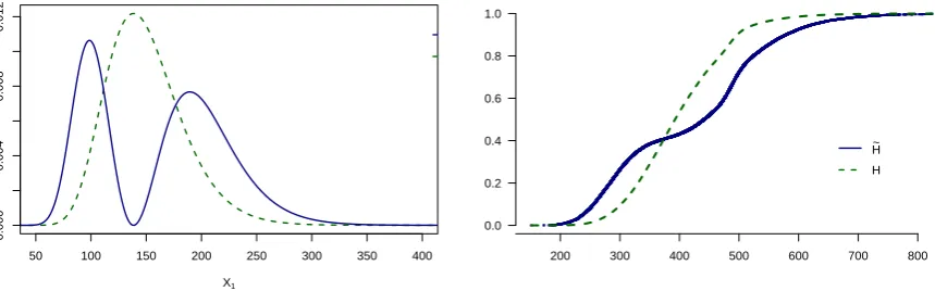
Example (non-linear insurance portfolio continued). To calculate the cascade sensitivity, the
importance sampling routine of this section can be employed, where the distorted densities
˜
fi, i= 1,2, are given by
˜
fi(x) =
x−m x
1 +ln(x)−µ
σ2
fi(x), x >0. (8)
The left plot in Figure 3 shows the importance weights f˜1(X1)
f1(X1) against the input factor X1.
Note that the importance weights are zero at the mode of X1 and give more weight to high