A bi-level programming approach for trip matrix estimation and traffic control problems with stochastic user equilibrium link flows

This is a repository copy of A bi-level programming approach for trip matrix estimation and traffic control problems with stochastic user equilibrium link flows.

White Rose Research Online URL for this paper: http://eprints.whiterose.ac.uk/2459/

Article:

Maher, M.J., Zhang, X. and van Vliet, D. (2001) A bi-level programming approach for trip matrix estimation and traffic control problems with stochastic user equilibrium link flows. Transportation Research Part B : Methodological, 35 (1). pp. 23-40. ISSN 0191-2615 https://doi.org/10.1016/S0191-2615(00)00017-5

[email protected] https://eprints.whiterose.ac.uk/ Reuse

See Attached

Takedown

If you consider content in White Rose Research Online to be in breach of UK law, please notify us by

White Rose Research Online

Institute of Transport Studies

University of Leeds

This is an author produced version of a paper published in Transportation

Research Part B. It has been uploaded with the permission of the publisher. It has been refereed but does not include the publisher’s formatting or pagination.

White Rose Repository URL for this paper: http://eprints.whiterose.ac.uk/2459/

Published paper

Maher M.J., Zhang X. and van Vliet D. (2001) A bi-level programming approach for trip matrix estimation and traffic control problems with stochastic user

equilibrium link flows. Transportation Research Part B : Methodological, 35(1), 23-40

A BI-LEVEL PROGRAMMING APPROACH FOR TRIP MATRIX ESTIMATION

AND TRAFFIC CONTROL PROBLEMS WITH STOCHASTIC USER

EQUILIBRIUM LINK FLOWS

MICHAEL J.MAHER andXIAOYAN ZHANG

School of Built Environment, Napier University,

10 Colinton Road, Edinburgh EH10 5DT UK

and

DIRCK VAN VLIET

Institute for Transport Studies, Leeds University, Leeds LS2 9JT UK

Abstract ⎯ This paper deals with two mathematically similar problems in transport network

analysis: trip matrix estimation and traffic signal optimisation on congested road networks.

These two problems are formulated as bi-level programming problems with stochastic user

equilibrium assignment as the second-level programming problem. We differentiate two types

of solutions in the combined matrix estimation and stochastic user equilibrium assignment

problem (or, the combined signal optimisation and stochastic user equilibrium assignment

problem): one is the solution to the bi-level programming problem and the other the mutually

consistent solution where the two sub-problems in the combined problem are solved

simultaneously. In this paper, we shall concentrate on the bi-level programming approach

although we shall also consider mutually consistent solutions so as to contrast the two types

of solutions. The purpose of the paper is to present a solution algorithm for the two bi-level

programming problems and to test the algorithm on several networks.

Keywords: Trip matrix estimation, Traffic signal optimisation, Stochastic user equilibrium

1. INTRODUCTION

In this paper, we deal with two mathematically similar problems in transport network

analysis: trip matrix estimation and traffic signal optimisation on congested road networks.

These two problems are of great importance in transport planning, scheme appraisal and

traffic management. A matrix estimation problem and signal optimisation problem have a

common input: route choice proportions or, equivalently, link flows in the road network.

These are the output of a traffic assignment model which, in turn, requires a trip matrix or

signal settings as inputs. An equilibrium assignment (EA) model needs to be included in the

matrix estimation and signal optimisation so as to achieve consistency in route choices and to

model congestion effects in the network. This can either be a user equilibrium (UE)

assignment model or a stochastic user equilibrium (SUE) assignment model. In the combined

matrix estimation and EA problem, there are two linked optimisation problems: matrix

estimation (ME) problem with fixed route choice proportions and the EA problem with a

fixed trip matrix. Similarly in a combined signal optimisation and EA problem, there are also

two linked optimisation problems: the signal optimisation (SO) problem with fixed link flows

and the EA problem with fixed signal settings. In both combined problems, there is a mutual

interaction between the two sub-problems.

In recent years there has been increasing interest in formulating the two combined problems

as bi-level programming (BP) problems (Bard, 1988) in which the ME or the SO problem is

at the upper level and the EA problem at the lower level. A BP problem has a hierarchical

structure in which an upper-level and a lower-level decision maker must select their strategies

so as to optimise their objective functions, respectively. But, the upper-level decision maker

knows how the lower-level optimiser would react to a given upper-level decision and acts

accordingly while the lower-level optimiser can act only according to given decisions of

upper-level problem. On the other hand, a conventional approach to deal with the two

combined problems is to treat the two sub-problems in a parallel way and to seek a mutually

consistent solution. This "mutually consistent" problem falls into another type of

mathematical programming problem, namely, the equilibrium programming (EP) problem

(Garcia and Zangwill, 1981). In an EP problem, each of the two parties is continuously

The BP problem is different from the EP problem in that the upper-level decision maker

knows how the lower-level decision maker makes a decision. Although he cannot intervene in

the lower-level decision maker's decision, he can consider the lower-level decision maker's

reaction in his own decision making. This is particularly important in the bi-level signal

optimisation problem. In the EP problem, on the other hand, neither of the two optimisers

knows how the other would react; each of them acts only according to the decision of the

other. In this paper, we shall concentrate on the BP approach although we shall also consider

mutual consistent solutions so as to contrast the two types of solutions.

The BP problem may be seen as a single programming problem with the upper-level variables

being constrained by the lower-level solutions. In this sense, a BP problem is similar to a

non-linear programming (NP) problem. However, in a BP problem, the evaluation of the

upper-level objective function requires solving the lower-upper-level optimisation problem whose

functional form is generally unknown. A further complication is that a BP problem is in

general non-convex. This implies the potential existence of local minimum solutions and so a

global minimum may be difficult to find. The EP problem is similar to a multiple-objective

NP problem in that there are two objectives. However, in a NP problem, there is only one

decision maker who chooses all variables so as to optimise several objectives. In an EP

problem, on the other hand, there are two decision makers, each having control of only one

set of variables. (A more general EP problem can have more than two parties.) It is clear that

most standard algorithms for NP problems may not be applicable to BP and EP problems.

The two types of programming problem may also be cast into the framework of game theory.

Fisk (1984) discussed a range of combined problems in the framework of game theory, and

the discussion was illustrated by the combined signal optimisation and UE assignment

problem. In game theory, a mutually consistent solution corresponds to a Nash

non-cooperative game and a BP problem to a Stackelberg game or leader-follower game. In fact,

the Nash non-cooperative game is a special type of EP problem. Formulating the two

combined problems as different types of mathematical programming problems or games can

help to understand the nature of the problems. However, solution algorithms developed in

these theories may not be applicable to general transport network problems because a

O-D pairs. Most algorithms developed for the two combined problems in transport networks

have been heuristic. These methods will be reviewed later in the paper.

Recently, the authors have developed algorithms for the solution of the combined ME and UE

assignment problem, and of the combined SO and UE assignment problem (Zhang & Maher,

1998; Maher & Zhang, 1999). In this paper, we present a solution algorithm for the bi-level

matrix estimation problem, and the bi-level signal optimisation problem, using the new

algorithm for the logit-based SUE assignment model by Maher (1998). The two combined

problems will be discussed separately in sections 2 and 3, each of which contains the problem

formulation, the algorithm and the test results. The SUE algorithm will be described in

subsection 2.3 before the proposed bi-level solution algorithm is described. The paper is

summarised in the last section.

2. THE COMBINED MATRIX ESTIMATION AND SUE ASSIGNMENT PROBLEM

2.1. The problem formulation and the solution

The problem of trip matrix estimation has been considered by many researchers (e.g.,

Cascetta and Nguyen, 1988). One of the most widely used formulations for matrix estimation

is the minimisation of the weighted sum of squared distances between the observed and

estimated traffic flows (Cascetta, 1984):

ME: Min _ME(t,v) (t t)U 1(t t) (v v)W 1(v v)

t = − − + − −

− −

Z (1)

subject to v=Pt, t≥0

where

ZME is the objective function for matrix estimation;

t is the vector containing the trip matrix to be estimated, t=(…, ti, …), i∈I;

I is the set containing O-D pairs;

tis the vector of the target matrix, t=(…, ti, …), i∈I;

v is the vector containing the observed link flows, v =(…, va, …), a∈A ;

A is the subset of links with observed link flows, A⊆A;

A is the set of links in the network;

U and W are weighting matrices, or the variance-covariance matrices of target matrix and the

observed link flows;

P is the matrix containing proportions of each O-D flow using each link, or link choice

proportions.

All vectors in this paper are column vectors. Note that the second term of the objective

function is defined only for those links with traffic counts; it is not necessary to have all the

links in the network observed. In the matrix estimation problem, t is the set of decision

variables, v varies with t, and P is assumed to be given. The solution to this problem, t*, is

the generalised least squares (GLS) estimator and is given by (Cascetta, 1984)

) (

) +

(

= U 1 P W 1P 1 U 1t P W 1v

t∗ − T − − − + T − (2)

The link flows and link choice proportions are determined from a trip assignment model. We

shall use the optimisation formulation for SUE assignment proposed by Powell and Sheffi

(1982):

SUE:

∑

∑

∑ ∫

∈ ∈

− +

− =

A a

v

a A

a

a a a i

i i

a

x x c v

c v S

t Z

0

SUE( , ) ( ) ( ) ( )d

Min v t v

v

where ca (va) is the cost-flow function for link a and Si is the value of the satisfaction function

of O-D pair i arising from a stochastic loading based on link flow v. In the SUE assignment

problem, it is possible to find a SUE solution of link choice proportions together with link

flows. Although we have included the trip matrix t in the objective function, t is fixed in the

SUE assignment problem. In this section, we will use V(t) and P(t) to denote SUE solutions

of link flows and link choice proportions. Then we have V(t)=P(t)t. It worth mentioning that

SUE assignment does not in general have an explicit functional form of V(t) or P(t), not even

The bi-level trip matrix estimation problem is one in which the matrix estimator tries to

minimise the matrix estimation error while the link flow pattern adjusts itself accordingly to a

SUE. The problem may be written as

(4a) )

) ( , (

Min _ME t P t t

t

t∈D Z

or

(4b) ))

( , (

Min _ME t V t

t

t∈D Z

where Dt is the feasible regions for t, V(t)=P(t)t, and V(t) is the lower-level SUE assignment

problem. The EP formulation of the problem, on the other hand, is

(5a) )

, ( Min _ME t Pt

t

t∈D Z

(5b) )

, ( Min _SUE v t

v

v∈D Z

where Dv is the feasible regions for v. Note the difference between (4a) and (5a): the former is

solved with variable P while the latter with fixed P. It is clear that the mutually consistent

solution is also a feasible solution of the bi-level problem. The two solutions are in general

different and the bi-level solution has a smaller value of the ME objective function than that

of the mutually consistent solution. By definition, among all the solutions that satisfy SUE

conditions, the bi-level solution has the minimum ME objective function value.

2.2. Previous solution algorithms for the combined problem

Hall et at. (1980) considered a combined ME and UE problem, in which the observed link

flows are assumed to be error-free. An iterative algorithm for solving the problem was

proposed, in which the two sub-problems are solved alternatively until convergence is

achieved. This iterative estimation-assignment (IEA) algorithm has been widely used.

depending on whether the coupling between the two sub-problems is weak or not. In addition,

when it does converge, it will converge to the mutually consistent solution. Yang et al. (1992)

and Yang (1995) considered a more general bi-level trip matrix estimation problem with UE

assignment at the lower level. They proposed two heuristic algorithms which also involve

alternate optimisation of the upper- and lower-level problems. The first algorithm is

essentially the same as that by Hall et at. (1980) mentioned above, though the algorithm is

developed for solving the more general problem. The second algorithm involves calculating

the gradient using a sensitivity analysis method (Tobin and Friesz, 1988) to obtain the partial

derivatives of UE link flows with respect to O-D flows. It has been shown (Maher and Zhang,

1999) that, at least in a two-link network, the first algorithm converges to the mutually

consistent solution while the second algorithm to the bi-level solution. In general, however,

conditions for the convergence of both algorithms remain to be proved. An example in which

the IEA algorithm diverges in a two-link network example was also shown in Maher and

Zhang (1999).

Below, we describe a solution algorithm for the bi-level problem. But before that we describe

the algorithm for logit-based SUE assignment, which is a basic building block for the bi-level

solution algorithm.

2.3. Algorithm for logit-based SUE assignment

The solution to the SUE problem is an iterative process. At each iteration a search direction is

found by carrying out a stochastic loading based on travel costs calculated from the current

link flows, v(k). Then the link flows are updated by

v(k+1) =v(k)+λ(k)(u(k)−v(k))

where λ(k) is the step length taken along the search direction (u(k)−v(k)), and u(k) is the auxiliary

solution obtained from a stochastic network loading. Different algorithms differ in the way

the step length is determined. In the method of successive average (MSA), a sequence of

predetermined step lengths is used: λ(k)=1/(k+1) (Powell and Sheffi, 1982). The algorithm

optimal step length is calculated at each iteration. A stochastic loading carried out with the

current link flow v(k) will produce not only the auxiliary flow pattern u(k), but also the value of

the satisfaction function {Si(v(k))} and hence the value of the objective function ZSUE(v(k)).

Furthermore, the derivative of the objective function along the search direction at λ=0 can

also be obtained:

) ( d ) ( d ) ( d )) ( (

d ( ) ( ) ( ) ( )

0 SUE ) ( k a k a v v a a a a k a k

a u v

v v c u v Z k a a − − = = =

∑

Another stochastic loading at the auxiliary solution point will give rise to another pair of the

objective function value ZSUE(u(k)) and the derivative:

) ( d ) ( d ) ( d )) ( (

d ( ) ( ) ( ) ( )

1 SUE ) ( k a k a u v a a a a k a k

a u v

v v c w u Z k a a − − = = =

∑

where w(k)={wa(k)} is the auxiliary flow pattern from a stochastic loading based on link flow

u(k). Quadratic or cubic interpolation along the search direction can then be used to derive an

estimate of the optimal step length (i. e. that at which ZSUE is minimum or each component of

the gradient is zero).

The logit stochastic loading algorithm considers only efficient links so as to avoid explicit

route enumeration (Dial, 1971). However, when the stochastic loading is used as part of a

SUE algorithm, the set of efficient links for each O-D pair may vary from iteration to iteration

as link flows and costs vary. Consequently, the objective function is not necessarily

continuous and convergence of the algorithms may be affected. One way round this difficulty

is to make the choice of a set of efficient links based on some predetermined link flow pattern

(such as free-flows) and to maintain the same set of efficient links throughout the iterative

process (Leurent, 1997).

Suppose we have a current solution, [t(n),v(n)], where v(n)=V(t(n)). At each iteration, the

upper-level problem is firstly solved to get an auxiliary solution of the trip matrix, t*, assuming

v=PP

(n)

t. Then, a SUE assignment is performed to find the SUE link flows, v*, or V(t*) at t*.

Thus, we have two points satisfying SUE conditions, t(n) and t*. We then search for an

optimal step length along (t*−t(n)) by a line search. In the bi-level problem (4a) or (4b),

however, a line search directly based on the objective function requires repeated SUE

assignment and is very inefficient. To overcome this difficulty, we linearise the SUE

assignment map between the two points, (t(n),v(n)) and (t*,v*), that is

V(t) ≅ v(n)+Q(t−t(n))

where Q=[Qai] and Qai=(va*−va(n))/(ti*−ti(n)). Let

t(β)=t(n)+β(t*−t(n)) (6a)

We have

v(β)=v(n)+β(v*−v(n)) (6b)

Then an optimal step length β* can be found by minimising ZME(t(β),v(β)). This is a standard

one-dimensional search and can be solved by, for example, the Newton method. The function

ZME(t(β),v(β)) and its derivatives with respect to β can be evaluated for any value of β. The

first and the second derivatives of the ZME(t(β),v(β)) with respect to β are

) )( ), ( ( ) )( ), ( ( d )) ( ), ( (

d ME (n) (n)

F F Z v v v v t t t t v t v v t

t − +∇ −

∇

= _β ∗ _β ∗

β β β ) )( ), ( ( ) ( ) )( ), ( ( ) ( d )) ( ), ( ( d ) ( 2 ) ( ) ( 2 ) ( 2 2 ME n T n n T n F F Z v v v v v v t t t t t t v t v v t t − ∇ − + − ∇ − = ∗ ∗ ∗ ∗ β β β β β

The new solution of the trip matrix is then given by (6a) with β*. However, v(β*) obtained by

(6b) is only an approximation to V(t(β*)). Therefore, another SUE assignment is performed

The SUE solution itself is an iterative process. Therefore, there are two nested iterations in

the algorithm for the bi-level solution: the outer iterations for the bi-level solution and the

inner iterations for the SUE solution. We shall use free-flow costs to determine a set of

efficient links and use this set throughout both inner iterations for SUE assignment and outer

iterations for the bi-level solution. The bi-level algorithm can be outlined as follows.

Step 1: Determine a set of efficient links by carrying out a stochastic loading based on free-flow link costs.

Step 2: Initialise t(0), v(0), and PP

(0)

; set n=0. The initial trip matrix can normally be set to be the target matrix. Assigning the target matrix to the network by SUE assignment gives v(0) and P(0)P .

Step 3: Determine a GLS estimation of t* by equation (2), using v=PP

(n) t. Step 4: Find V(t*) for t* by carrying out a SUE assignment.

Step 5: Find β which minimises ZME(t(β),v(β)) by, for example, the Newton method. Step 6: Set t(n+1)=t(n)+β(t*−t(n)).

Step 7: Find v(n+1) = V(t(n+1) as well as PP

(n+1)

(t(n+1) by carrying out another SUE assignment. Step 8: If the convergence criterion is met, stop; otherwise, set n:=n+1 and go to step 3.

The stopping criterion can be based on the maximum relative change in the elements of the

estimated trip matrix at successive iterations:

Maxi (|ti(n+1)− ti(n))|/ ti(n)) ≤ε

where ε is the error tolerance. This stopping criterion may not be a good indicator of an

optimal solution. Another possible stopping criterion is the change of objective function

values at successive iterations. However, due to the nonlinearity and nonconvexity of the

problem, it is possible for different solutions to have similar objective function values. In the

following numerical tests of the algorithm, the above stopping criterion is used to terminate

the iterative process, and the changes in objective function values are also observed to make

sure that the changes are also small.

Several comments need to be made about the algorithm. First, although we have considered

the GLS method for matrix estimation, other methods, such as the entropy maximisation

method, can also be used without changing the structure of the algorithm. Second, this

algorithm needs two SUE assignments at each iteration. This is necessitated by the bi-level

can be made more efficient by starting the SUE assignment with the latest link flow pattern

rather than the free-flow pattern. For example, at Step 4, the initial link flows for SUE

assignment can be set to be v=PP

(n)

t*. Third, in this algorithm, the auxiliary solution does not

necessarily point to a descent direction and the optimal step length is not limited to be

positive. Fourth, the algorithm involves an approximation in the optimal step length

calculation: the SUE assignment map is linearised over the interval between the current and

the auxiliary solution. The interval is generally finite because the auxiliary solution does not

in general become closer to the current solution with increasing iteration number. Thus there

is no reason to expect that the linearisation will become more and more accurate as the

algorithm converges. As a result, the algorithm may converge to some point in the

neighbourhood of the true solution due to the approximation. This problem may be dealt with

by reducing the interval between the current and the auxiliary solution of matrix by, for

example, a MSA-type scheme so that the linearisation is made over a smaller and smaller

interval. This can be implemented by replacing the auxiliary solution of matrix with

t(n)+(t*−t(n))/n at the end of step 3 of the bi-level algorithm. It can be expected that the

algorithm will become less efficient with this modification. Numerical tests with the networks

tried so far have shown that the first few iterations of the algorithm are most "cost effective";

the solution is close to the optimal one after only a few iterations. Therefore, if higher

accuracy is desirable, we can introduce the modification after the first few iterations when the

solution is close to optimal or when the ME objective function is not reduced at further

iterations. The improvement of the algorithm can be observed by the reduction in the value of

objective function of matrix estimation. This modification procedure will be demonstrated in

the numerical calculations below.

2.4. Test results

There are two parts in this test. In the first part a simple example is used to test if the

algorithm can identify the bi-level solution because in this example the bi-level solution can

be found by direct search. The network has one O-D pair connected by two links The cost

functions on the two links are

c2 = 6.25 + v2/1000

The target matrix is t =2000 and the link count is ₁ v =620, made on link 2. The value of ₂

"spread parameter" θ in the logit model used is 0.5, and an error tolerance ε is 0.001. These

two values will be used for all numerical tests in this paper. The solutions by the bi-level

algorithm, and the modified level algorithm at the 20th iteration, together with the true

bi-level solution and the mutually consistent solution are shown in Table 1. The modification to

the bi-level solution was introduced after three initial iterations of the original algorithm when

the iterations have passed the convergence test. The true solution was found by direct search

in the trip matrix with an incremental size of 0.001 ⎯ a more detailed search showed that the

objective function is rather flat and does not change much with changes in the matrix at the

fourth decimal place. The mutually consistent solution was found by the IEA algorithm. It can

be seen that the bi-level algorithm gives a good approximation to the true bi-level solution

and that the modification improves the accuracy of the algorithm, though only marginally. It

can also be seen that the bi-level solution has a smaller value of ZME than that of the mutually

consistent solution, as expected.

{Table 1 is about here}

The second part of the experiment is made to investigate the performance of the algorithm for

different values of errors in the prior matrix and the observed links flows on two networks. In

this test, the true trip matrix is supposed to be known. Assigning the true matrix to the

network by SUE assignment gives the true link flows. The target matrix and the observed link

flows are generated by (Yang et al., 1992)

) 0

. 1 ( ~

od i v i

i t C

t = − ξ

) 0

. 1 ( ~

lk a v a

a v C

v = − ζ

where ti

~

and v~ are the elements of the true matrix and link flows, ξa i and ζa are randomly

random errors of the target matrix and observation errors in link flows respectively. The

variance-covariance matrices, U and W, are assumed to be diagonal matrices with the

variances (Yang et al., 1992)

Var(t )=(C_i vod ti

~ )2

Var( v )=(C_a vlk v~ )a

2

The BPR (Bureau of Public Roads) cost function will be used:

⎥ ⎦ ⎤ ⎢

⎣ ⎡

+

= _α γ

) ( 1 ) 0 ( ) (

a a a

a a

q v c

v c

where [ca(0)] is uncongested link costs, [qa] is link capacity, and α and γ are constants. The

values α=1.0 and γ=4.0 will be used. We shall show the results calculated on two networks

and then analyse the results.

The first network is the grid network shown in Figure 1. The network has 9 nodes and 24

links. There are 4 centroids (nodes 1, 3, 5, and 7) and 4 O-D pairs (1→5, 3→7, 5→1, 7→3).

The true matrix is assumed to be: [72 60 72 60]. The uncongested link costs [ca(0)] and link

capacities [qa] are listed in Table 2. Calculations with different values of Cvod and Cvlk are

summarised in Table 3, including the solutions and the values of objective functions at the

20th iteration of the algorithm, the number of iterations as well as the c.p.u. times (in seconds)

needed for the algorithm to converge at the given error tolerance. Also shown in the table is

the mutually consistent solutions found by the IEA algorithm. In addition, convergence of the

proposed algorithm in terms of objective function values with the largest values of Cvlk is

shown in Figure 2. The second test was made on the well-known Sioux Falls network.

Information in the data set includes the network characteristics (link-node topology and the

parameters in the cost functions) and a demand trip matrix which is treated as the true matrix.

The network has 76 links, 24 nodes. All nodes are both origins and destinations, and so there

are 576 O-D pairs. The values of objective functions at the 20th iteration of the algorithm, the

number of iterations as well as the c.p.u. times (in seconds) needed for the algorithm to

summarised Table 4. Convergence of the algorithm in terms of objective function values is

shown in Figure 3.

{Figure 1 is about here}

{Table 2 is about here}

{Table 3 is about here}

{Figure 2 is about here}

{Table 4 is about here}

{Figure 3 is about here}

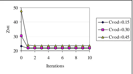
Several points can be observed from the results. First, the proposed algorithm converges after

a few iterations and is quite efficient. Second, the two types of solutions are different and the

value of the objective function of the matrix estimation problem is lower at the bi-level

solution than that at the mutually consistent solution. Third, the larger the errors in the prior

matrix and observed link flows, the more effort it takes for the algorithms to converge.

Fourth, the computation time of the algorithms also depends on the size of a network. The

calculations were made on a 300MHz Pentium II machine with 64.0 Mb RAM. Whilst an

estimation takes about 2-3 minutes to converge on the Sioux Falls network, it takes only one

or two seconds for the iterations to converge on the grid network at the same error tolerance.

The main computational burden in the proposed algorithm is the solution of the ME problem

itself an iterative process. If there are many more O-D pairs than links, such as in the Sioux

Falls network, the solution of the ME problem contributes more significantly to the c.p.u.

time. On the other hand, if there are a lot more links than O-D pairs, such as in the grid

network, SUE assignment contributes more significantly to c.p.u. time.

3. THE COMBINED SIGNAL OPTIMISATION AND SUE ASSIGNMENT PROBLEM

3.1. The problem formulation and previous algorithms

The combined signal optimisation and SUE assignment problem is mathematically similar to

that of the combined matrix estimation and SUE assignment (Note that the trip matrix is

assumed to be fixed in the signal optimisation problem). The most commonly used policy for

signal optimisation is to minimise the total journey costs in the network:

SO: )Min _SO( , )= _a( _a, _a

A a

a c v s v Z

∑

subject to samax≥ sa≥ samin, a∈A

s_a a Aj

= ∈

∑

where sa is the ratio of green for link a, s=(…, sa, …); samax and samin are maximum and

minimum allowable green split for link a, samin>0, samax<1; Aj is the set of links heading for

the jth signal controlled intersection. If link a is not controlled by a signal, then samax, sa, and

samin will all be equal to 1. The set of link flows v is the output from a SUE assignment

problem. Given a signal setting, s, the SUE assignment problem (3) may be re-written as

SUE:

∑

∑

∑ ∫

∈ ∈ − + − = A a v a a A a a a a a i i i a x s x c s v c v S q Z 0

SUE( , ) ( ) ( , ) ( , )d

Min v s v

v

In this section, we will use V(s) to denote the SUE link flows for given s. The bi-level

)

)

) ) ( , ( min

Arg SO

BL

s V s s

s

s∈D Z =

while a mutually consistent solution, [sMC, vMC], can be expressed as

, ( min

Arg _SO MC

MC

v s s

s

s∈D Z =

, ( min

Arg MC

SUE MC

s v v

v

v∈D Z =

The comparison of the two types of solutions here is the same as that in the combined matrix

estimation and SUE assignment problem. However, it is important to note that the bi-level

solution has a smaller value of SO objective function which is the total cost in the network.

Therefore, the system would perform better under bi-level approach.

The traffic signal optimisation problem is a special case of the more general optimal network

design problem, in which the number of phases, the cycle time, and the offsets of traffic

signals are determined. The optimal network design problem has been considered by many

researchers (See e.g., Davis, 1994; Friesz et. al., 1992; Harker and Friesz, 1984; Suwansirikul

et. al., 1987 among others). In this paper, we consider signal optimisation for isolated

intersections. Thus, given a set of link flows, the SO problem is reduced to several

sub-problems of determining the optimal green split for each signal controlled intersection. Each

of them may be solved by any standard one-dimensional optimisation algorithm, such as the

Newton method.

An iterative algorithm in which the SO and UE problems are solved alternately has been used

for the solution of the combined SO and UE problem (Van Vuren and Van Vliet, 1992; Smith

and Van Vuren, 1993). As in the matrix estimation problem, this iterative optimisation-

assignment (IOA) procedure may converge to the mutually consistent solution but

convergence is not guaranteed (Fisk, 1984, 1988). Several types of algorithms have been

proposed for the solution of the bi-level signal optimisation problem with UE assignment

(Sheffi and Powell, 1983; Heydecker and Khoo, 1990; Yang and Yagar, 1995). See Maher

and Zhang (1999) for a review for these algorithms. However, these algorithms require

repeated UE assignment for direction finding and/or for line search. Using MSA instead of a

algorithms. Cascetta et al. (1998) considered a combined signal optimisation and SUE

assignment problem. They proposed two methods for direction finding. The first one is the

opposite gradient direction identified by numerical differentiation. This needs several SUE

assignments, as in the method by Sheffi and Powell (1983). The second method is the use of

the solution of the SO problem with fixed link flows as a direction. This, however, does not

necessarily provide a descent direction. The step lengths calculation is a modified MSA

algorithm in which step size is reduced only when the objective function is not reduced.

3.2. The proposed algorithm and the test results

The algorithm proposed here is similar to that for trip matrix estimation, with the trip matrix

estimation being replaced by signal optimisation with fixed link flows. The algorithm will not

be repeated here but the method of line search is described briefly. The optimal step length is

found by solving

) ) ( , ) ( (

Min _SO β β

β Z s v

subject to β∈[βmin,βmax]

where

s(β)=s(n)+β(s*−s(n))

v(β)=v(n)+β(v*−v(n))

and [βmin,βmax] is determined from constraints on signal parameters and link flows. The line

search can be solved by the bisection method and no stochastic loading is needed. The first

derivative of the objective function with respect to β needed in the bisection method is given

by ) ( ) ( ) ( = ) ) ( , ) ( ( d

d ( ) ( )

SO

∑

∑

∈ ∈ ∗ ∗ ₋ ∂ ∂ + − ∂ ∂ + A

a a C

n a a a a a n a a a a a

a s s

s c v v v v c v c

Z β β

The algorithm is tested on two networks. The cost function used is a combination of the BPR

function (for link travel time) and the signal delay formula by Doherty (1977), that is

a a a a a a d q v c v

c _⎥+

⎦ ⎤ ⎢ ⎣ ⎡ +

= _α γ

) ( 1 ) 0 ( ) (

Here da is signal delay for link a and is given by

a a a a a a a a v s q v s q s T d − + −

= (1 ) 1980 2

2

, va /(qa sa)≤0.95

2 2 ) ( 3600 220 3600 55 . 198 ) 1 (

2 _{a a}

a a a a a s q v s q s T

d = − − × + × , va /(qa sa)>0.95

where T is the cycle time and is fixed at 90 seconds in the test. The values of α=1.0 and

γ=4.0 are used in the BPR function.

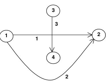
The first test was made on a simple three-link network shown in Figure 4. The network has

two O-D pairs, with demand t1 = t2 = 100. O-D pair 1 is connected by link 1 and link 2. O-D

pair 2 is connected by link 3. There is a signal at the intersection of links 1 and 3. The

uncongested link costs [ca(0)] and link capacities [qa] are

[ca(0)] = [1 2 1]

[qa] = [200 100 200]

Direct search (by exhaustive trial of all possible solutions of signal settings, with increment

size of 0.0001) has shown that in this example, there is only one optimal bi-level solution and

that the solution is s1=0.3070. Three initial signal splits for s5 are used in the test: 0.3, 0.5, and

0.7; and the algorithm converges to the same solution. The solutions by the bi-level algorithm,

and the modified bi-level algorithm (modification introduced at the fourth iteration) at the

20th iteration, together with the true bi-level solution found by direct search and the mutually

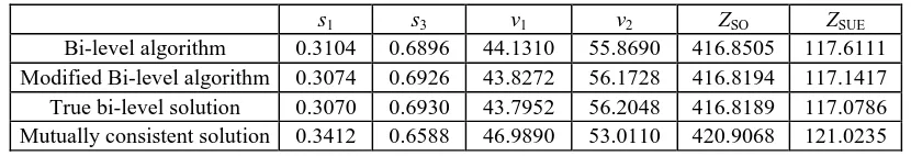
consistent solution found by the IOA algorithm are summarised in Table 5. It can be seen that

the bi-level algorithm converges almost to the true bi-level solution and that the modification

its capacity is comparable to that of link 1 (considering signal control). More drivers would

naturally use link 1 at low demand. However, if the signal optimiser knows drivers' route

choice behaviour, as in the bi-level problem, he can reduce the green split on link 1 and thus

divert more traffic to link 2. Therefore, we have in Table 5 s1BL<s1MC; v1BL<v1MC; and the total

cost, ZSO, in the bi-level solution is lower than that in the mutually consistent solution.

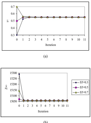
Another similar test was carried out on the same grid network as shown in Figure 1 used for

the matrix estimation problem. A traffic signal is added at node 9 and the capacities on all

links controlled by the signal (links 5, 10, 15, 20) is doubled. The convergence of the green

splits and the objective function values with the three initial values of s5 are shown in Figure

5. It can be seen that the bi-level algorithm is very efficient. In fact, in just a few iterations,

the algorithm converges to [s5, s10] = [0.5506, 0.4494] with ZSO=15058.3954, which is the

same as the true bi-level solution found by direct search in the signal split with increment size

of 0.0001. Therefore, in this case, the modification to the bi-level algorithm is not necessary.

{Figure 4 is about here}

{Table 5 is about here}

{Figure 5 is about here}

4. SUMMARY

The problem of combined trip matrix estimation and SUE assignment, and that of traffic

signal optimisation and SUE assignment have been addressed in this paper. Two types of

solutions are identified and compared. An algorithm for the bi-level solution of the two

problems has been described. At each iteration, the algorithms use standard routines of matrix

search is made by linearising the SUE assignment model, which does not need repeated SUE

assignments.

The algorithm was tested on simple two- or three- link networks, a 3×3 grid network with 24

links and 4 O-D pairs, and the Sioux Falls network with 24 nodes, 76 links, and 528 O-D

pairs. It was shown to be convergent and efficient in terms of the number of iterations and

c.p.u. times. In the two- or three- link network examples in which the true bi-level solution

can be found by direct search, it was shown that the bi-level algorithm converges almost

exactly to the true bi-level solution. The errors are caused by the linearisation of the SUE

map. A modification to the algorithm is proposed and has been shown to be effective.

The algorithm presented here is heuristic in nature. It has not been possible to prove

theoretically that the algorithm is convergent. In addition, it is not guaranteed that the

algorithm identifies the global optimal even when it does converge. Fletcher (1987) argued

that the existence of convergence proof for any algorithm is not a guarantee of good

performance in practice; and the development of an algorithm also relies on experimentation.

The algorithm presented here has been used to solve the bi-level ME problem with UE

assignment or logit-based SUE assignment at the lower level, and the bi-level SO problem,

again with UE assignment or logit-based SUE assignment at the lower level. The networks

tested so far include simple two- or three-link networks, 3×3 grid networks, the Sioux Falls

network and the Headingley network. The last two networks are used in the congested ME

problems only. The Headingley network has 73 nodes, 188 links, and 240 O-D pairs. Test on

this network can be found in Zhang et. al., 1999. In all the tests so far it has been found that

the algorithm is convergent. In those cases where the (global) optimal solution can be found

by direct search (two- or three-link networks or the grid network with one traffic signal), it

was found that the algorithm is able to identify or to give a good approximation of the optimal

solutions. Further tests of the algorithm on more general networks will be carried out.

Because of its simplicity, the logit assignment model has been most widely used. However, it

has well-known weaknesses. For example, it does not take account of overlapping or

correlated routes. Cascetta et al. (1996) have proposed a modified logit model which allows

for overlapping routes, but the model requires complete route enumeration. On the other

and Hughes (1997) have developed a probit-based SUE assignment algorithm which does not

require route enumeration. Further work of the current research is to adapt the bi-level

algorithm for use with probit-based SUE assignment.

Acknowledgement⎯The authors are grateful to the UK Engineering and Physical Science

Research Council for funding the work reported in this paper, and to three anonymous

referees who made valuable, constructive suggestions for the improvement of the paper.

References

Bard, J. F. (1988). Convex two-level optimisation. Mathematical Programming, 40, 15-27.

Cascetta, E. (1984). Estimation of trip matrices from traffic counts and survey data: a

generalised least squares estimator. Transportation Research, 18B, 289-299.

Cascetta, E., Gallo, M. and Montella, B. (1998). Models and algorithms for the optimisation

of signal settings on urban networks with stochastic assignment. Sixth Meeting of the

EURO Working Group on Transportation, 9-11 September, 1998, School of

Mathematics and Computing Sciences, Chalmers University of Technology,

Gothenburg, Sweden.

Cascetta, E. and Nguyen S. (1988). A unified framework for estimating or updating

origin/destination matrices from traffic counts. Transportation Research, 22B,

437-455.

Cascetta, E., Nuzzolo, A., Russo, F. and Vitetta, A. (1996). A modified logit route choice

model overcoming paths overlapping problems, specifications and some calibration

results for interurban networks. Proceedings of the 13th International Symposium on

Transportation and Traffic Theory (J. B. Lesort editor), Pergamon, 697-711.

Davis, G. A. (1994). Exact local solution of the continuous network design problem via

stochastic user equilibrium assignment. Transportation Research, 28B, 61-75.

Dial, R. B. (1971). A probabilistic multipath traffic assignment model which obviates path

enumeration. Transportation Research, 5, 83-111.

Doherty A. R. (1977). A comprehensive junction delay formula. LTRI Working Paper,

Fisk, C. S. (1984). Game theory and transportation systems modelling. Transportation

Research, 18B, 301-313.

Fisk, C. S. (1988). On combining maximum entropy trip matrix estimation with user optimal

assignment. Transportation Research, 22B, 69-79.

Fletcher, R. (1987). Practical methods of optimisation, Second edition. John Wiley & Sons

Ltd.

Friesz, T. L., Cho, h., Mehta, N. J., Tobin, R. L. and Anandalingam, M. (1992). A simulated

annealing approach to the network design problem with variational inequality

constraints. Transportation Science, 26, 18-26.

Garcia, C. B. and Zangwill, W. I. (1981). Pathways to Solutions, Fixed Points, and

Equilibria. Prentice-Hall, Inc., Englewood Cliffs.

Hall, M. D., Van Vliet, D. and Willumsen, L. G. (1980). SATURN: A simulation assignment

model for the evaluation of traffic management schemes. Traffic Engineering and

Control, 21, 168-176.

Harker, P. T. and Friesz, T. L. (1984). Bounding the solution of the continuous equilibrium

network design problem, Proceedings of the 9th International Symposium on

Transportation and Traffic Theory (J. Volmuller and R. Hamerslag Editors), VNU

Science Press, The Netherlands, 233-252.

Heydecker, B. G. and Khoo, T. K. (1990). The equilibrium network design problem.

Proceedings of AIRO’90 Conference on Models and Methods for Decision Support,

Sorrento, pp 587-602.

Leurent, F. M. (1997). Curbing the computational difficulty of the logit equilibrium

assignment model. Transportation Research, 32B, 315-326.

Maher, M. (1998). Algorithms for logit-based stochastic user equilibrium assignment.

Transportation Research, 32B, 539-549.

Maher, M. J. and Hughes, P. C. (1997). A probit-based stochastic user equilibrium

assignment model. Transportation Research, 31B, 341-355.

Maher, M. J. and Zhang, X. (1999). Algorithms for the solution of the congested trip matrix

estimation problem. Transportation and Traffic Theory, Proceedings of the 14th

International Symposium on Transportation and Traffic Theory (A. Ceder, Editor),

Elsevier, 445-469.

Powell, W. B. and Sheffi, Y. (1982). The convergence of equilibrium algorithms with

Sheffi, Y. and Powell, W. B. (1983). Optimal signal setting over transportation networks.

Transportation Engineering, 109, 824-839.

Smith M. J. and Van Vuren, T. (1993). Traffic equilibrium with responsive traffic control.

Transportation Science, 27, 118-132.

Suwansirikul, C., Friesz, T. L. and Tobin R. L. (1987). Equilibrium decomposed optimisation:

a heuristic for the continuous equilibrium network design problem. Transportation

Science, 21, 254-263.

Tobin R. L. and Friesz, T. L. (1988). Sensitivity analysis for equilibrium network flows.

Transportation Science, 22, 242-250.

Van Vuren T. and Van Vliet, D. (1992) Route Choice and Signal Control. Athenaeum Press

Ltd., Newcastle upon Tyne.

Yang, H. (1995). Heuristic algorithms for the bi-level origin-destination matrix estimation

problem. Transportation Research. 29B, 1-12.

Yang, H., Sasaki, T., Iida, Y. and Asakura Y. (1992). Estimation of origin-destination

matrices from link traffic counts on congested networks. Transportation Research,

26B, 417-434.

Yang H. and Yagar, S. (1995). Traffic assignment and signal control in saturated road

networks. Transportation Research, 29A, 125-139.

Zhang, X. and Maher, M. (1998). An algorithm for the solution of bi-level programming

problems in transport network analysis. Mathematics in Transport Planning and

Control (J. D. Griffiths, Editor), Elsevier, 177-186.

Zhang, X., Maher, M. and Van Vliet, D. (1999). Methods for the solution of the combined

trip matrix estimation and stochastic user equilibrium assignment problem. To be

presented on European Transport Conference, 27-29 September, 1999, Cambridge,

TABLES

Table 1. Solutions of the matrix estimation problem on the two-link network

t1(20) v1(20) P1(20) ZME(20) ZSUE(20)

Bi-level algorithm 1937.1100 1170.4515 0.604226 25463.8575 -9022.1208

Modified bi-level algorithm 1937.1157 1170.4548 0.604226 25463.8574 -9022.1506 True bi-level solution 1937.1160 1170.4550 0.604226 25463.8574 -9022.1507 Mutually consistent solution 1941.2442 1172.8129 0.604155 25484.0922 -9043.4699

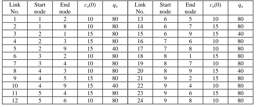
Table 2. Uncongested link travel costs and link capacities on the grid network.

Link No.

Start node

End node

ca(0) qa Link

No.

Start node

End node

ca(0) qa

1 1 2 10 80 13 6 5 10 80

2 1 8 10 80 14 6 7 15 80

3 2 1 15 80 15 6 9 15 40

4 2 3 15 80 16 7 6 10 80

5 2 9 15 40 17 7 8 10 80

6 3 2 10 80 18 8 1 15 80

7 3 4 10 80 19 8 7 10 80

8 4 3 10 80 20 8 9 15 40

9 4 5 15 80 21 9 2 15 80

10 4 9 15 40 22 9 4 10 80 11 5 4 15 80 23 9 6 15 80 12 5 6 10 80 24 9 8 10 80

Table 3. Performance of the matrix estimation algorithm on the grid network with ε=0.001.

Bi-level solution algorithm Mutually consistent solution

Cvlk Cvod t1(20) t2(20) t3(20) t4(20) ZME(20) c.p.u. N t1(20) t2(20) t3(20) t4(20) ZME(20)

Table 4. Performance of the matrix estimation algorithm on the Sioux Falls network with

ε=0.001.

Bi-level solution algorithm Mutually consistent solution

Cvlk Cvod ZME(20) c.p.u. N ZME(20)

0.05 0.05 39.4834 57.58 2 39.7423

0.05 0.10 41.8604 84.34 3 42.9385

0.05 0.15 44.3356 85.16 3 46.4643

0.10 0.10 39.4407 67.09 2 39.6997

0.10 0.20 41.7600 84.56 3 42.8199

0.10 0.30 44.1281 86.54 3 46.2565

0.15 0.15 39.4084 88.46 3 39.6667

0.15 0.30 41.6537 86.43 3 42.7068

0.15 0.45 43.9314 89.01 3 46.1082

Table 5. Solutions of the signal optimisation problem on the three-link network.

s1 s3 v1 v2 ZSO ZSUE

FIGURES

1 2 3

4

5 6

7

8 9

Figure 1. The grid network. All links are two-directional.

20 30 40 50

0 2 4 6 8 10

Iterations

Z

ME

Cvod=0.15

Cvod=0.30

Cvod=0.45

Figure 2. Convergence of the matrix estimation algorithm on the grid network, with Cvlk=

35 45 55 65

0 2 4 6 8 10

Iterations

Z

ME

Cvod=0.15

Cvod=0.30

Cvod=0.45

Figure 3. Convergence of the matrix estimation algorithm on the Sioux Falls network, with

Cvlk= 0.15.

1

3

1 2

3

4

2

0.3 0.4 0.5 0.6 0.7

0 1 2 3 4 5 6 7 8 9 10 11

Iteration

s

5

(a)

15050 15100 15150 15200 15250 15300

0 1 2 3 4 5 6 7 8 9 10 11

Iteration

Z

SO

S5=0.3

S5=0.5

S5=0.7

(b)