Boosting Boosting

Boosting Boosting

Thesis by

Ron Appel

In Partial Fulfillment of the Requirements for the degree of

Doctor of Philosophy

CALIFORNIA INSTITUTE OF TECHNOLOGY Pasadena, California

2017

© 2017

Ron Appel

ACKNOWLEDGEMENTS

I would like to thank:

Pietro Perona – as an academic mentor, for teaching me, allowing and encouraging me to work on problems that interest me, and for being patient with me through my stubbornness – and as a friend, for your kindness, your calm, your humor, and your heartfelt, sound advice in matters of life outside of academia.

My lab mates and non-lab mates – for all the fun times, all the love and support, all the help in stressful situations; I could not have found a better group of friends.

ABSTRACT

Machine learning is becoming prevalent in all aspects of our lives. For some appli-cations, there is a need for simple but accurate white-box systems that are able to train efficiently and with little data.

“Boosting” is an intuitive method, combining many simple (possibly inaccurate) predictors to form a powerful, accurate classifier. Boosted classifiers are intuitive, easy to use, and exhibit the fastest speeds at test-time when implemented as a cas-cade. However, they have a few drawbacks: training decision trees is a relatively slow procedure, and from a theoretical standpoint, no simple unified framework for cost-sensitive multi-class boosting exists. Furthermore, (axis-aligned) decision trees may be inadequate in some situations, thereby stalling training; and even in cases where they are sufficiently useful, they don’t capture the intrinsic nature of the data, as they tend to form boundaries that overfit.

My thesis focuses on remedying these three drawbacks of boosting. Ch. 3 outlines a method (called QuickBoost) that trains identical classifiers at an order of magnitude faster than before, based on a proof of a bound. In Ch. 4, a unified framework for cost-sensitive multi-class boosting (called REBEL) is proposed, both advancing theory and demonstrating empirical gains. Finally, Ch. 5 describes a novel family of weak learners (called Localized Similarities) that guarantee theoretical bounds and outperform decision trees and Neural Nets (as well as several other commonly used classification methods) on a range of datasets.

PUBLISHED CONTENT AND CONTRIBUTIONS

[1] R. Appel, X. P. Burgos-Artizzu, and P. Perona. “Improved Multi-Class Cost-Sensitive Boosting via Estimation of the Minimum-Risk Class”. In: arXiv 1607.03547 (2016). URL: arxiv.org/abs/1607.03547

Ron conceived and carried out the project, with help from Xavier on some experiments. Co-authors helped in writing the paper.

[2] R. Appel and P. Perona. “A Simple Multi-Class Boosting Framework with Theoretical Guarantees and Empirical Proficiency”. In: International Con-ference on Machine Learning(2017). [Accepted]

Ron conceived, carried out the project, and wrote the paper.

[3] R. Appel et al. “Quickly boosting decision trees-pruning underachieving fea-tures early”. In:International Conference on Machine Learning(2013). Ron conceived and carried out the project. Co-authors helped write the paper.

[4] P. Dollár, R. Appel, and W. Kienzle. “Crosstalk Cascades for Frame-Rate Pedestrian Detection”. In:European Conference on Computer Vision(2012). Ron implemented fast feature extraction code and helped write the paper.

[5] P. Dollár et al. “Fast Feature Pyramids for Object Detection”. In:IEEE Trans-actions on Pattern Analysis and Machine Intelligence(2014).

TABLE OF CONTENTS

Acknowledgements . . . iv

Abstract . . . v

Published Content and Contributions . . . vi

Table of Contents . . . vii

Notation . . . viii

Chapter I: Introduction . . . 1

Chapter II: Machine Learning . . . 6

2.1 Learning to Predict . . . 7

2.2 Boosting . . . 13

Chapter III: Quickly Boosting Decision Trees . . . 19

3.1 Introduction . . . 19

3.2 Related Work . . . 20

3.3 Boosting Trees . . . 21

3.4 Pruning Underachieving Features . . . 27

3.5 Experiments . . . 30

3.6 Conclusions . . . 33

Chapter IV: Cost-Sensitive Multi-Class Boosting . . . 36

4.1 Introduction . . . 36

4.2 Related Work . . . 38

4.3 Approach . . . 40

4.4 Decision Trees . . . 45

4.5 Weak Learning Conditions . . . 46

4.6 Experiments . . . 49

4.7 Discussion . . . 55

4.8 Conclusions . . . 56

Chapter V: Theoretically Guaranteed Learners . . . 59

5.1 Introduction . . . 59

5.2 REBEL Revisited . . . 61

5.3 Binarizing Multi-Class Data . . . 63

5.4 Isolating Points . . . 65

5.5 Generalization Experiments . . . 67

5.6 Comparison with Other Methods . . . 73

5.7 Discussion . . . 75

5.8 Conclusions . . . 76

Chapter VI: Conclusions . . . 78

Chapter VII: Appendices . . . 80

7.1 Statistically Motivated Derivation of AdaBoost . . . 80

7.2 QuickBoost via Information Gain, Gini Impurity, and Variance . . . 82

7.3 Reduction of REBEL to Binary AdaBoost . . . 86

NOTATION

R Set of real numbers(_−∞,_∞)

R Set of extended real numbers[_−∞,_∞] (i.e. including_±∞) Px,y Joint probability distribution (i.e. P(x, y))

Py|x Posterior probability distribution (i.e.P(y|x))

x Scalar (non-bold font)

f(_·) Scalar function (i.e. returns a scalar)

1(...) Indicator function, returns1if logical expression (represented as “...”) evaluates to true, otherwise returns0

x Vector (boldfont)

0 Zero vector (i.e. [0,0, ...,0])

1 One vector (i.e. [1,1, ...,1])

δδδk Indicator vector (i.e. 0with a1in thekthindex)

H(_·) Vector-valued function (i.e. returns a vector)

xk Value of thekthindex in vectorx (i.e. xk≡ hx, δδδki)

C Matrix (Bold Underlinedfont)

ha,b_i Inner product ofaandb

a⊙b Element-wise product ofaandb(i.e.[a

1b1, a2b2, ..., aKbK])

exp[x] Element-wise exponentiation (i.e.[ex1_{, e}x2_{, ..., e}xK]₎

g[x] Square brackets indicate element-wise function (i.e.[g(x1), g(x2), ..., g(xK)]) ˜

y Estimate (tilde-hat) of a quantityy

Chapter 1

INTRODUCTION

The year is 2017 and we have just recently entered the age of machine learning. Algorithms that automatically analyze data are indispensable tools and are being heavily applied in all aspects of our lives. Companies are competing to hire machine learning experts to properly implement these algorithms. However, such powerful tools should be accessible to all members of society, not just the experts. With this body of work, I propose a simple framework that is ready to deploy with the push of a button, no expertise necessary. But first, I recount a brief history of events that motivated my work.

At the turn of the (21st_{) century, the first object detection system capable of}

function-ing in real-time was proposed: the Viola-Jones face detector [14]. One of the main aspects of computer vision is object detection, i.e. finding and/or identifying a par-ticular object within in image or video frame. As humans, faces are prevalent in our daily lives and hence are particularly relevant as detectable “objects”, marking the Viola-Jones detector as a major milestone. The detector was intuitively clear and easily implementable, largely owing its success to the “brains” behind its operation: the machine learning system, namely,boosting[7].

Boosting was able to produce very good visual object classifiers by combining many simple features (e.g. the average pixel intensity of a rectangular image patch). In-deed, methods based on boosting remained state-of-the-art in many fields for over a decade [6, 3, 1]. However, the good times didn’t last; in 2012, AlexNet [9] paved the way for the resurgence of neural networks, leaving boosting almostforgotten. As of this year, deep nets of varying (obscenely large and complex) architectures have taken over, reaching almost if not better than human performance in many domains [10].

One of the key strengths of these networks is their ability to transform the input data by learning complex feature representations to facilitate classification [12]. How-ever, there are several considerable drawbacks to employing such networks.

allowed to run autonomously only if it couldexplainits every decision and action. Further, when used towards the scientific analysis of phenomena (e.g. understand-ing animal behavior, weather patterns, financial market trends, etc.), the goal is to extract a causal interpretation of the system in question; hence, to be useful, a machine should be able to provide a clear explanation of its internal logic.

To demonstrate the potential flaws in the almost magical inner-workings of deep nets, Fig 1.1 is borrowed from [13]. Seemingly identical inputs are classified as completely different classes (in both cases, with high reported levels of confidence). [13] claims that every sample can be appropriately adjusted to be classified as any class. Although these adjustments are very specific, the fact remains that the more complex the network, the more mysterious its functionality.

Subtle adjustments to random samples from Imagenet images and MNIST digits

Figure 1.1: (Results from [13]) (left) Random Imagenet images [5], correctly classified samples (top row), incorrectly classified subtly adjusted samples (middle row), and the amplified pixel-wise difference between the two seemingly identical images (bottom row). (right) Random MNIST digits [11], correctly classified sam-ples (odd columns), incorrectly classified subtly adjusted samsam-ples (even columns).

For these reasons, it is desirable to have a simple white-box machine learning sys-tem that can train quickly and with little data. To this end, I have sped up train-ing time, theoretically unified and empirically improved cost-sensitive multi-class boosted classification, and have proposed better constituents for use in the overall boosted classifier. My proposed boosting framework is the accurate, data-efficient, easy-to-use tool that should be in everyone’s tool-bag.

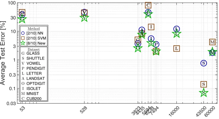
To demonstrate its versatility, Fig. 1.2 shows a plot of test error rates on ten datasets ranging in amount of training dataN, input sample dimensionalityd, and number of output classesK, (refer to Table 1.1 for specifications). I compare my proposed method to neural networks (trained using four different architectures: [d₋4d₋K], [d₋4K₋K], [d₋2d₋d₋K], [d₋4K₋2K₋K], finally reporting the one that performed best on the test set) and SVMs (support vector machines [4] – another standard machine-learning method; cross-validating to find optimal parametersC andγ using a5_×6grid search)1. As described above, the neural nets and SVMs required several runs in order to select appropriate hyper-parameters. My method did not require validation and led to the best accuracy in almost all cases. It is decisively the best choice of algorithm based on these results.

53 ₅₂₈

38234435559462387494 _{16000 4350060000}

Number of Training Samples (N₎

0.03 0.1 0.3 1 3 10 30 100

Average Test Error [%]

G G G S S S V V V P P P L L L A A A O O O I I I M M M C C C [2/10] NN [2/10] SVM [8/10] New

GLASS SHUTTLE VOWEL PENDIGIT LETTER LANDSAT OPTDIGIT ISOLET MNIST CUB200 G S V P L A O I M C Method Dataset

Figure 1.2: Comparison of my (New) method versus neural networks and support vector machines on ten datasets of varying sizes and difficulties. My method is the most accurate on almost every dataset.

1

10-2 10-1 100 101 102

Average Error of My Method [%]

10-2 10-1 100 101 102

Average Error of SVM and NN [%]

G G

S

S

V V

P

P L

L A A

O

OI

I

M M

C C

NN SVM

Figure 1.3: Comparison of error rates achieved using my method versus neural net-works and support vector machines on ten datasets of varying sizes and difficulties. Note that almost all of the points lie in the top-left half of the plot, signifying that my method is the most accurate method on almost every dataset.

# Input # Output # Training # Test

Dataset dims. classes samples samples

GLASS 9 6 53 159

SHUTTLE 9 7 43500 14500

VOWEL 10 11 528 462

PENDIGIT 16 10 7494 3498

LETTER 16 26 16000 4000

LANDSAT 36 6 4435 2000

OPTDIGIT 64 20 3823 1797

ISOLET 617 26 6238 1559

MNIST 728 10 60000 10000

CUB200 4096 200 5594 5794

References

[1] N. Asadi and J. Lin. “Training Efficient Tree-Based Models for Document Ranking”. In:European Conference on Information Retrieval. 2013.

[2] K. Bache and M. Lichman.UCI Machine Learning Repository (UC Irvine). 2013.URL:http://archive.ics.uci.edu/ml.

[3] X.P. Burgos-Artizzu et al. “Social Behavior Recognition in continuous videos”. In:CVPR. 2012.

[4] C. Cortes and V. Vapnik. “Support-vector networks”. In:Machine Learning (1995).

[5] J. Deng et al. “ImageNet: A Large-Scale Hierarchical Image Database”. In: CVPR. 2009.

[6] P. Dollár, R. Appel, and W. Kienzle. “Crosstalk Cascades for Frame-Rate Pedestrian Detection”. In:ECCV. 2012.

[7] Y. Freund and R. E. Schapire. “A desicitheoretic generalization of on-line learning and an application to boosting”. In:European Conference on Computational Learning Theory. 1995.

[8] Y. Jia et al. “Caffe: Convolutional Architecture for Fast Feature Embedding”. In:arXiv1408.5093 (2014).

[9] A. Krizhevsky, I. Sutskever, and G. E. Hinton. “Imagenet classification with deep convolutional neural networks”. In:NIPS. 2012.

[10] Y. LeCun, Y. Bengio, and G. E. Hinton. “Deep learning”. In:Nature Research (2015).

[11] Y. LeCun and C. Cortes.The MNIST database of handwritten digits. Tech. rep. 1998.

[12] Y. LeCun et al. “Gradient-based learning applied to document recognition”. In:Proceedings of the IEEE(1998).

[13] C. Szegedy et al. “Intriguing properties of neural networks”. In:arXiv1312.6199 (2013).

[14] P. Viola and M. J. Jones. “Robust Real-Time Face Detection”. In: IJCV (2004).

[15] P. Welinder et al.Caltech-UCSD birds 200. Tech. rep. 2010.

Chapter 2

MACHINE LEARNING

Whether or not we believe in a higher power, we can all agree that there is a certain order to our existence (however chaotic it might be). This “order” in our world is the governing laws of nature (many of which we are still uncovering) and the “chaos” is the stochasticity – or randomness – inherent in every process. These laws (which can be thought of as pre-defined patterns or phenomena) ensure that for a given set of input conditions, we can expect a specific set of output results. The scientific method itself is based on this notion of repeatability – if the same procedure is repeated multiple times, similar results should occur.

All living entities thrive from being able to leverage these patterns, if not by fully comprehending them then at least by being able to predict them. More importantly, we are able to generalize our specific experiences to the infinite number of possible experiences that we have not already explicitly encountered.

As an example, from birth, we are subject to the pull of gravity, without knowing what it is. We notice that if we don’t hold ourselves up, we fall. If we let go of a ball, it falls. So does a piece of paper, although not as fast. Without having to grab and drop every object around us, we come to expect that all objects fall when released, some quickly and some slowly. And then on our birthday, we are given a helium balloon. We let it go and it immediately soars up and out of reach (and we cry). But we quickly learn to correctly predict which objects fall quickly, slowly, and which don’t fall at all – even without having to hold them first!

This learning mechanism is not intrinsic to animals, it can be achieved in machines as well, hence the termMachine Learning: training/teaching computers to predict (i.e. having them learn) the structure and/or input-output relationships based on previously-observed patterns.

We start by inspecting a number of samples (e.g. objects of various kinds); for each sample, we record the values of its input features (color, mass, and volume) and corresponding outputclass(whether it falls quickly, slowly, or floats). This set of samples is thetraining data, which is then analyzed using a pre-chosen algorithm. The “machine” crunches the data, attempting to extract the underlying input-output relationships. Upon completion, a new classifier is returned; able to hypothesize the class of any object given only its input features.

But how does this work? And which algorithm should we use? There are many to choose from, each resulting in different types of classifiers. In the following sections, we give a more formal perspective of machine learning, briefly overview various existing families of algorithms, and go into more detail on one specific family: the focus of our work,boosting.

2.1 Learning to Predict

Algebraically, we can represent any object as a set ofdfeatures, just as we did in the example above. Note that in general, an “object” can refer to any form of entity that we are dealing with (e.g. a digital image, bouts of animal behavior, financial trends, etc.; not necessarily a physical object). Accordingly, we abstract any such entity as ad-dimensional vector x, with each dimension encoding the value of some corre-sponding feature. Note that categorical (i.e. nominal) features can be represented as numerical features by assigning a discrete index to each category. As such, we define the input spaceXas the region of the overall space _Rd _{in which the data is} concentrated:

x_∈X_⊆Rd

Similarly, we can represent any output properties in which we are interested (i.e. observations) as aK-dimensional vectory, and defineYas the output space1:

y_∈Y_⊆RK

We assume that there is an underlying “order” to our existence, encoded as the prob-abilistic distributionPΩ. By marginalizing over all variables that do not compriseX

orY(i.e. ignoring all variables that are not input features or output observations), we definePx,y as the distribution that governs the layout and density of our specific input and output data.

Our high-level goal is to determine a functionH :X _→ Ythat accurately predicts the outputy given a specific input x, i.e. H(x) _≈ y. To characterize the perfor-mance of this function, we need to define a notion of error. Leterrbe some appro-priate measure of error between a predictiony˜ _≡ H(x)and an expected outputy. Accordingly, we can define the expected errorεE:

εE ≡ Ex,y

err H(x),y (2.1)

The lower the expected error, the more accurate the predictor. However, the joint spaceX_×Y(i.e. all possible input-output combinations) may consist of an infinite number of points, each with corresponding probabilities that cannot be explicitly computed. So how do we gauge this error? The best we can do is analyze a finite subset by gatheringN points and consolidating them into a datasetS. Collecting data in an unbiased way is equivalent to sampling from the joint distributionPx,y:

S _{≡ {}(xn,yn)}Nn=1 ∼ Px,y

With this dataset in hand, we can compute the corresponding empirical errorεS:

εS ≡ 1

N

N

X

n=1

err H(xn),yn

(2.2)

Throughout this work, we assume that our empirical error is agood enough approx-imation of the expected error: εS ≈ εE. There is a lot of formal math rigorously

defining the notion of “good enough”; however, it is outside the scope of our work. Please refer to [1] for a more comprehensive discussion on the topic.

Unsupervised Learning

In many situations, we only have access to the input points _{xn}, not their cor-responding outputs _{yn}. This could happen if the output observations or class labels are very difficult or impossible to obtain or are simply hidden from us. These situations constitute the Unsupervised Learningregime, so-named because no su-pervision (i.e. labels or expected outputs) are provided.

data into more meaningful feature representations (e.g. Self-Organizing Maps [16] and t-Distributed Stochastic Neighborhood Encoding(tSNE)[17]), to name a few.

However, throughout this work, we assume that we do have access to fully labeled data, or all ofS. Accordingly, our work focuses on theSupervised Learningregime. In this regime, we can still carry out any of the methods mentioned above, but we can also perform two other important tasks: regression and classification.

Regression

Back to our falling objects example, given only the color, mass, and volume of an object, we can try to predict the amount of time it takes that object to fall when dropped from a height of 1 m. In this case, our training setS consists of a scalar-valued output observationyn, namely, the falling time associated with each object

n. A pre-chosen regression method crunches the data, attempting to extract the un-derlying input-output relationships. Upon completion, a newregressoris returned, able to estimate the falling time of any object given only its input feature values.

More concretely, a regressorHestimates the value of one or more output observa-tions (dependent variables)ygiven the input features (independent variables)x:

H:X_→Y such that: H(x)_≈y

To quantify the accuracy of H, we make use an error function err, as in Eq. 2.1. A correct estimate should always incur zero error. In the case of regression, the larger the estimate relative to the expected output, the worse the error should be; similarly, the smaller the estimate relative to the expected output, the worse the error should be. Many different functions achieve this goal. Depending on the specific problem, some may be more suitable than others. Arguably the most intuitive and mathematically-simple function used for regression is the squaredL2norm between

an estimate and its expected output:

err(˜y,y)_{≡ k}y˜₋y_k2

Classification

attempting to extract the underlying input-output relationships. Upon completion, a newclassifieris returned, able to hypothesize the class of any object given only its input feature values.

More formally, a classifierF hypothesizes the class labelygiven input featuresx:

F :X_→Y such that: F(x)_≈y

In the context of classification, the output class is represented as an integer. For instance, if there areK possible classes, the output spaceYcan be defined as:

Y _{≡ {}1,2, ...,K_}

Quantifying the error of a classifier is different than that of a regressor. A class label is a discrete quantity; thus, there is no smooth notion of “almost” – a hypothesis is either right or it is wrong2. Accordingly, an apt error function for use in Eq. 2.1 is the misclassification indicator (error = 0 for the right answer, error = 1 for wrong):

err(˜y, y) _≡ 1(y˜6=y)

Estimating the Underlying Distributions

Recall our assumption that there exists an intrinsic order, encoded as a distribution Px,y over the joint input-output spaceX×Y. Given a specific inputx, the posterior distributionPy|xcan be computed using Bayes’ theorem:

P(y_|x) _≡ PP(x, y)

k∈Y

P(x, k)

Our goal is to understand the very phenomenon that is being described by these distributions; thus, by definition, we do not know them and so we cannot directly evaluate them. However, if weweresomehow able to evaluatePy|xfor anyxandy, wecouldclassify any given pointxas the class corresponding to the highest poste-rior probability. This (purely theoretical) strategy guarantees optimal classification, yielding the lowest possible expected error, i.e. theBayes classifierF∗:

F∗(x) _≡ arg max

y∈Y {P(y|x)} (2.3)

2_{Actually, some mistakes may be better (or less severe) than others. This scenario is known as}

But as we have just asserted, we cannot directly accessPy|x in practice. Fortunately, we can make use of our dataset Sto form an empirical estimateP˜, using this esti-mate as a basis for aMaximum A Posteriori(MAP) classifierF:

F(x) _≡ arg max y∈Y{

˜

P(y_|x)_} (2.4)

Being a finite dataset (i.e. having onlyN discrete points), we need to generalize over the entire input-output space. To this end, several approaches exist.

Non-parametric methods generalize the labels of discrete data points to their sur-roundings [21]. Kernel Density Estimation uses a pre-chosenkernelto smooth the discrete points in S so that they cover a much larger range of the problem space. Using K-Nearest Neighbors, the estimated posterior probability of a query point depends on distances from theK closest points inSand their corresponding labels. Similarly, Random Ferns use an ensemble of random input-space-hashing functions (i.e. ferns), each with a corresponding empirical posterior distribution, averaging them to form an overall estimate [18].

Alternatively, parametric models, explicitly defined over the entire space, can be used to estimate the joint distribution (and hence also the posterior distribution). Using Bayesian-style methods (e.g. Naive Bayes), model parameters are optimized to maximize the likelihood of the dataset [13].

With these estimation techniques, the choice of kernel or model can be rather heuris-tic, especially when little is known about the underlying structure of the problem. Regardless, the act of classification requires making a specific decision. In deter-mining the maximala posterioriclass (as in Eq. 2.4), a probability estimate is used only in relative comparisons; its absolute value is unimportant. This fact is particu-larly apparent when there are few classes.

Binary Classification

In the special case ofbinaryclassification (i.e. whenK= 2), we are distinguishing between the smallest possible number of distinct classes: two. Accordingly, data is typically split into two, a positiveand a negativeset, and the output space Yis commonly defined as:

Y _{≡ {±}1_}

The binary MAP classifier (i.e. the two-class equivalent of Eq. 2.4) reduces to:

F(x) _≡

(

+1, P˜(y= +1_|x)>1/2

−1, P˜(y= +1_|x)_≤1/2 ≡ sign ˜P(y= +1|x)−1/2

Note that the estimateP˜y|x may itself be inaccurate due to various sources of error: poor model selection, dataset bias, and unaccounted noise, to name a few. Moreover, classification is simply the comparison between the probability and a single fixed threshold (e.g. 1/2in Eq. 2.5). Consequently, requiring the estimator to be a valid probabilistic distribution may add unnecessary constraints and complexity.

Estimating Class Boundaries

Instead of applying the indirect procedure offirstestimating the posterior andthen classifying using MAP, we can ignore probabilities entirely and focus directly on decision boundaries. After all, this is what any classifier essentially reduces to.

Linear models split the input space into two using a hyperplane (i.e. a comparison between the weighted average of feature values and a threshold). Logistic Regres-sion [6] and Perceptron Learning [12] train (i.e. fine-tune) the hyperplane weights to improve the separation between positive and negative data points.

In many cases, the given input features are not ideal for linear classification. Rather than using these feature directly, we can apply various non-linear transformations to them to generate a new, potentially more suitablerepresentationof the data, thereby leading to more expressive classifiers.

Support Vector Machines (SVMs) work with a kernelization (i.e. a user-defined high-dimensional non-linear transformation) of the input data [7], maximizing the margin (i.e. minimum distance) between points of differing classes with a hyper-plane in the kernel (transformed) space. Instead of requiring a user-defined kernel (i.e. a hand-codedfeature transform), Neural Networks infer a transform from the data itself. This transform is implemented using multiple layers of interconnected perceptrons (i.e. linear projections followed by a non-linear transform) [15], and is optimized to facilitate more accurate classification.

Using multiple hyperplanes, Decision Trees divide the input space intoleaves(i.e. non-overlapping regions), each with a specific class label [19]. Assigning a label to a given query point involves a set of comparisons, starting at the root node (i.e. the trunk of the tree) and traversing through the branches – depending on the outcome of each comparison – until finally reaching a leaf node3.

The methods described above lead to learners (i.e. regressors or classifiers) that can function on their own. Some learners are more accurate and some are less

so. However, by appropriately combining the predictions of an ensemble of such learners, we can potentially improve (or boost) their individual accuracies. This “boosting” procedure is the focus of our work, and is described in greater detail in

the following section.

2.2 Boosting

Boosting is a beautifully simple yet effective procedure: given a set of relatively-poor classifiers (or weak learners), a strong classifier can be induced through a linear combination (i.e. a weighted sum) of their outputs. The basic procedure for boosting is intuitively described as follows:

1. Do your best: find (or train) the best weak learner given the original data (i.e. the learner that achieves the lowest training error as in Eq. 2.2).

2. Check your performance: based on the accuracy of the cumulative sum of previous learner(s), give more importance to individual samples that have incurred a larger error than to those with smaller error.

3. Focus on your mistakes: again, find (or train) a new weak learner, this time, accounting for the updated importance weights of the samples when deter-mining the corresponding error (see Eq. 2.11 below).

4. Keep on keepin’ on: repeat steps 2 and 3 until some satisfactory stopping condition is met.

One of the earliest and most popular algorithms for binary boosting is AdaBoost [11]. In the following sections, we motivate the AdaBoost algorithm from a prac-tical classification standpoint. AdaBoost can also be derived from a statisprac-tically- statistically-motivated standpoint; please see Appendix 7.1.

Greedily Minimizing a Surrogate Loss

In the context of binary classification, we are trying to generate a strong classifier F :X_{→ {±}1_}. Let us assume that we have a setFof binary weak learnersf:

F _{⊆ f}f :X→ {±1}

We define a confidence function h : X _{→ R} as a linear combination of T weak learners;ft∈Fare the learners andαt∈ Rare their corresponding weights:

h(x) _≡ T

X

t=1

The more weak learners individually agree with each others’ predictions, the further his from 0, and the more confidentthe prediction. Our strong classifierF simply predicts the more confident of the two possible labels; equivalent to the sign ofh:

F(x) _≡ sign h(x) (2.7)

With allT weak learners in the mix, the average training errorεis defined as:

ε _≡ 1

N

N

X

n=1

1(F(xn)6=yn) (2.8)

In this form, finding theT optimal(ft,αt)pairs is very difficult (if not intractable) for two reasons. Firstly, due to the indicator function, the errorεis non-convex in theT pairs(ft, αt). Secondly, this optimization requires an exponential number of operations (i.e. on the order of _|F_|T_{, where |F|is the number of weak learners in} the setF; potentially quite large).

To address the first issue, we use a convexsurrogateloss function_L. A valid loss should also upper-bound the training error, guaranteeing that error minimization is an implied consequence of loss minimization. The exponential functione−yh _is convex and upper-bounds the misclassification error for an individual point. It is the basis of AdaBoost, resulting in the following surrogate loss:

ε _{≤ L ≡} 1

N

N

X

n=1

e−ynh(x_n)

(2.9)

Note that: 1(sign(h)6=y)≤e

−yh _therefore:

L= 0 _⇒ ε= 0

To address the second issue, we apply agreedy, iterative training procedure. Instead of simultaneously optimizing all T learners, we “greedily” consider only the best one at each iteration. To start, we find the single best learnerf1. Holdingf1 fixed,

we find the best subsequent learnerf2. Then, holding all previously-chosen learners

fixed, we find the next one, and so on. This greedy procedure may be suboptimal due to its stage-wise nature, but it reduces the number of operations down to an order of only_|F_|·T, a tractable endeavor.

Optimal Weak Learner and Weight

Let’s assume that we have just trained the first I < T iterations. Consolidating Eqs. 2.9 and 2.6, the corresponding loss can be explicitly defined as:

LI = 1

N

N

X

n=1

exp₋yn I

X

t=1

αtft(xn)

The loss can be expressed as a sum of its current sample-wise constituentswn, re-ferred to as “sample weights” (not to be confused with weak learner weightsαt):

LI = 1

N

N

X

n=1

wn where: wn ≡ exp

−yn I

X

t=1

αtft(xn)

The sample weightwnsummarizes the cumulative performance of previously-chosen weak learners in classifying sample n; the worse the classification, the greater its weight (and vice-versa). Since all previous learnersftand weightsαtare held fixed due to the greedy training procedure, the next iteration’s loss_Lis defined as a func-tion of only thenextweak learnerf and corresponding weightα, as follows:

L(f, α) = 1

N

N

X

n=1

exp₋yn

_XI

t=1

αtft(xn) + αf(xn)

= 1 N N X n=1

exp₋yn I

X

t=1

αtft(xn)

| {z }

wn

e−α ynf(x_n) = 1

N

N

X

n=1

wne−α ynf(

x_n)

(2.10)

Since class labels and binary weak learner outputs can only be_±1, therefore:

incorrect classification: f(x)₆=y _⇒ e−α yf(x) =eα

correct classification: f(x) =y _⇒ e−α yf(x₎ =e−α

Furthermore, given a weak learnerf, the relative weighted errorεf is defined as the (weighted) proportion of samples that are incorrectly classified byf:

εf ≡ N

P

n=1

1(f(xn)6=yn)wn N

P

n=1

wn

= 1

N_LI N

X

n=1

1(f(xn)6=yn)wn (2.11)

∴ 1

N

N

X

n=1

1(f(xn)6=yn)wn = εf LI ∴ 1

N

N

X

n=1

1(f(xn)=yn)wn = (1−εf)LI

Accordingly, Eq. 2.10 can be expressed as the sum of two terms (misclassifications andcorrect classifications):

L(f, α) = e α

N

N

X

n=1

1(f(xn)6=yn)wn +

e−α

N

N

X

n=1

1(f(xn)=yn)wn = εfeα + (1−εf)e−α

Given a weak learnerf, the optimal corresponding weightα∗ is obtained by setting the derivative to zero and solving:

∂_L

∂α = 0 = εfe

α∗

− (1₋εf)e−α ∗

∴ e2α ∗

= 1−εf

εf

∴ α∗ = 1

2ln

_1−εf

εf

(2.12)

The AdaBoost surrogate loss (as in Eq. 2.9) not only leads to a simple, closed-form solution for the optimal learner weightα∗_{, but for the resulting loss as well:}

eα∗ =

r

1₋εf

εf

∴ L(f) =

εf

r

1₋εf

εf

+ (1₋εf)

r

εf 1₋εf

LI = 2√εf(1−εf)LI (2.13)

Consequently, the optimal weak learnerf∗ is the minimizer of the above loss. In practice, f∗ is determined by looping through and evaluating Eq. 2.14 for weak learnersf _∈F, finally recalling the best one.

f∗ = arg min

f∈F{L(f)} (2.14)

Training a Weak Learner

At each iteration, instead of passively finding the best weak learner from a set of predetermined learnersF, a weak learner can be specifically trained for use in the current iteration. Accordingly, any of the methods discussed in Sec. 2.1 can be used, appropriately modified to account for the specific sample weightswn(resulting from the previous boosting iterations).

In particular, shallow decision trees are easily trainable (refer to Sec 3.3) and have proven to be very suitable weak learners in practice, used in a multitude of domains such as computer vision, behavior analysis, and document ranking [9, 5, 2]. Shallow trees are also particularly quick to evaluate, enabling applications that require fast output speeds, especially when combined withcascades.

Cascaded Evaluation

Recall that a strong classifierF returns the sign of the confidence functionh:

F(x) _≡ sign h(x) where: h(x) _≡ T

X

t=1

Instead of evaluating allT weak learners, the final decision may already be deter-mined (with a high probability or even definitely) after onlyI < T learners:

F(x) _≈ sign hI(x) where: hI(x) _≡ I

X

t=1

ft(x)αt

This observation gives rise to the idea of cascaded evaluation: instead of accumulat-ing the confidence of allT learners at once, keep track of the cumulative confidence score. If a lower or upper threshold is reached before allT learners are evaluated, an early classification can be made. Thresholds are typically set by trading-off ac-curacy and aggressiveness of early termination (e.g. by finding upper and lower thresholds h±

t for which 95% of validation samples are correctly classified after only 10% of weak learners have been evaluated). As a result, early classification can be as accurate or aggressive as desired [3].

Accordingly, the following procedure (called soft cascades [3]) can be used to eval-uate a boosted classifier:

0. initialize to: t= 0, h= 0

1. incrementtand update the confidence score: t_←t+1, h_←h+ft(x)αt

2. if a lower or upper threshold is reached, return with the appropriate label (i.e. if h_≤h−

t then return F=−1, if h≥h

+

t then return F= +1)

3. if allT weak learners have been evaluated, return F= sign(h) otherwise, goto step 1.

Note that a simple extension to the above procedure is to repeat step 1 for a total of M times before continuing to step 2, thereby coarsening the cascade.

Boosting Boosting

The combination of simple weak learners and the potential for fast cascaded evalua-tion makes boosted shallow decision trees a very strong candidate for many machine learning tasks. In this work, we aim to further improve boosting by:

• Proposing a procedure for speeding up the training of decision trees (Ch. 3)

• Proposing a unified method for improved cost-sensitive multi-class boosting (Ch. 4)

References

[1] Y. S. Abu-Mostafa, M. Magdon-Ismail, and H.-T. Lin.Learning from data. AML-Book New York, NY, USA: 2012.

[2] N. Asadi and J. Lin. “Training Efficient Tree-Based Models for Document Ranking”. In:European Conference on Information Retrieval. 2013.

[3] L. Bourdev and J. Brandt. “Robust object detection via soft cascade”. In: CVPR. 2005.

[4] S. Branson, O. Beijbom, and S. Belongie. “Efficient Large-Scale Structured Learn-ing”. In:CVPR. 2013.

[5] X.P. Burgos-Artizzu et al. “Social Behavior Recognition in continuous videos”. In:

CVPR. 2012.

[6] M. Collins, R. E. Schapire, and Y. Singer. “Logistic Regression, AdaBoost and Breg-man Distances”. In: (2000).

[7] C. Cortes and V. Vapnik. “Support-vector networks”. In:Machine Learning(1995). [8] A. P. Dempster, N. M. Laird, and D. B. Rubin. “Maximum likelihood from

incom-plete data via the EM algorithm”. In:Journal of the royal statistical society(1977). [9] P. Dollár, R. Appel, and W. Kienzle. “Crosstalk Cascades for Frame-Rate Pedestrian

Detection”. In:ECCV. 2012.

[10] I. Fodor.A Survey of Dimension Reduction Techniques. Tech. rep. 2002.

[11] Y. Freund and R. E. Schapire. “A desicion-theoretic generalization of on-line learn-ing and an application to boostlearn-ing”. In: European Conference on Computational Learning Theory. 1995.

[12] Y. Freund and R. E. Schapire. “Large margin classification using the perceptron algorithm”. In:Machine Learning(1999).

[13] J. H. Friedman, T. Hastie, and R. Tibshirani. The elements of statistical learning. Springer, 2001.

[14] T. Kanungo et al. “An efficient k-means clustering algorithm: Analysis and imple-mentation”. In:PAMI(2002).

[15] Y. LeCun et al. “Backpropagation applied to handwritten zip code recognition”. In:

Neural Computation(1989).

[16] Y. Liu, R. H. Weisberg, and C. N. K. Mooers. “Performance evaluation of the self-organizing map for feature extraction”. In: Journal of Geophysical Research: Oceans(2006).

[17] L. J. P. van der Maaten and G. E. Hinton. “Visualizing High-Dimensional Data Using t-SNE”. In:Journal of Machine Learning Research(2008).

[18] M. Ozuysal et al. “Fast keypoint recognition using random ferns”. In:PAMI(2010). [19] J. R. Quinlan. “Induction of decision trees”. In:Machine Learning(1986).

[20] G. Shen, G. Lin, and A. van den Hengel. “StructBoost: Boosting methods for pre-dicting structured output variables”. In:PAMI(2014).

Chapter 3

QUICKLY BOOSTING DECISION TREES

Corresponding paper: [1]

Boosted decision trees are among the most popular learning tech-niques in use today. While exhibiting fast speeds at test time, rela-tively slow training renders them impractical for applications with real-time learning requirements. We propose a principled approach to overcome this drawback. We prove a bound on the error of a de-cision stump given itspreliminaryerror on a subset of the training data; the bound may be used to prune unpromising features early in the training process. We propose a fast training algorithm that exploits this bound, yielding speedups of an order of magnitude with no loss in the final performance of the classifier. Our method is not a new variant of boosting; rather, it is used in conjunction with existing boosting algorithms and other sampling methods to achieve even greater speedups.

3.1 Introduction

Boosting is a technique of combining many weak learners to form a single strong one [30, 17, 18]. Shallow decision trees are commonly used as weak learners due to their simplicity and robustness in practice [26, 5, 28, 22]. This powerful combina-tion (of boosting and decision trees) is the learning backbone behind many methods across a variety of domains such as computer vision, behavior analysis, and docu-ment ranking to name a few [11, 8, 2], with the added benefit of exhibiting very fast speeds at test time.

offers a speedup of an order of magnitude over prior approaches while maintaining identical performance.

Our contributions are the following:

1. Given the performance on a subset of data, we prove a bound on a stump’s classification error, information gain, Gini impurity, and variance.

2. Based on this bound, we propose an algorithm guaranteed to produce identi-cal trees as classiidenti-cal algorithms, and experimentally show it to be one order of magnitude faster for classification tasks.

3. We outline an algorithm for quickly boosting decision trees using our quick tree-training method, applicable to any variant of boosting.

In the following sections, we discuss related work, inspect the tree-boosting process, describe our algorithm, prove our bound, and conclude with experiments on several datasets, demonstrating our gains.

3.2 Related Work

Many variants of boosting [18] have proven to be competitive in terms of predic-tion accuracy in a variety of applicapredic-tions [7]; however, the slow training speed of boosted trees remains a practical drawback. A large body of literature is devoted to speeding up boosting, mostly categorizable as methods that subsample features or data points and methods that speed up training of the trees themselves.

In many situations, groups of features are highly correlated. By carefully choosing exemplars, an entire set of features can be pruned based on the performance of its exemplar. [12] propose clustering features based on their performances in previous stages of boosting. [21] partition features into many subsets, deciding which to inspect at each stage using adversarial multi-armed bandits. [25] use random pro-jections to reduce the data dimensionality, in essence merging correlated features.

Although all these methods can be made to work in practice, they provide no per-formance guarantees.

A third line of work focuses on speeding up training of decision trees. Building upon the C4.5 tree-training algorithm of [27], using shallow (depth-D) trees and quantizing features values intoB_≪Nbins leads to anO(D_×d_×N)implementation wheredis the number of features, andN the number of samples [34, 31].

Orthogonal to all of the above methods is the use of parallelization; multiple cores or GPUs. Recently, [32] distributed computation over cluster nodes for the applica-tion of ranking; however, reporting lower accuracies as a result. GPU implementa-tions of GentleBoost exist for object detection [9] and for medical imaging using Probabilistic Boosting Trees (PBT) [3]. Although these methods offer speedups in their own right, we focus on the single-core paradigm.

Regardless of the subsampling heuristic used, once a subset of features or data points is obtained, weak learners are trained on that subset in its entirety. Conse-quently, each of the aforementioned strategies can be viewed as a two-stage process; in the first, a smaller set of features or data points is collected, and in the second, decision trees are trained on that entire subset.

We propose a method for speeding up this second stage; thus, our approach can be used in conjunction with all the prior work mentioned above for even greater speedup. Unlike the aforementioned methods, our approach provides a performance guarantee: highly sped-up training with identical performance as classical training.

3.3 Boosting Trees

A boosted classifier (or regressor) having the form F(x) _≡ sign P_tαtft(x)

can be trained by greedily minimizing a loss function_L; i.e. by optimizingweak learner

ftand corresponding weightαtat each iterationt. Before training begins, each data sample n is assigned a non-negative weight wn (as discussed in Sec. 2.2). After each iteration, misclassified samples are weighted more heavily, thereby increasing the severity of misclassifying them in following iterations. Regardless of the flavor of boosting used (i.e. AdaBoost, LogitBoost, L2Boost, etc.), each iteration requires

Training Decision Trees

In the context of classification, a binary decision tree fTREE(x) processes an input

x and outputs a class label (either +1 or ₋1). Internally, the tree is composed of a decision stump (i.e. a two-way split) sj(x) at every non-leaf node j. Each stump corresponds to a binary decision, parametrized with a polarityp _{∈ {±}1_}, a thresholdτ _∈R, and a feature indexk _{∈ {}1,2, ...,d_}, and expects an inputx_∈Rd_:

sj(x) _≡ pjsign xkj−τj

where: xkj ≡ hx, δδδkji

s₂

s₄

s5

− + − +

s₃

s₆

s7

− + − +

s₁

Root Node

Branch Nodes

Leaf Nodes

Figure 3.1: A shallow (depth-3) binary tree. Each non-leaf node corresponds to a binary decision stumpsj(x). The output of a stump determines which stump is evaluated next: an output of +1 means the next stump is to the right, otherwise the next stump is to the left. Upon reaching a leaf node, the output of the tree corresponds to the output of the last stump to be evaluated.

Trees are commonly grown using a greedy procedure as described in [6, 27], re-cursively setting one stump at a time, starting at theroot node (i.e. the trunk) and working through to the extremities (i.e. the pre-leaf nodes). In this work, we focus on classification error; for other split criteria (e.g. information gain, Gini impurity, or variance), refer to Appendix 7.2 for similar derivations.

In the context of classification, the goal in each stage of stump-training is to find the optimal parameters that minimizeε, the average weighted classification error:

ε _≡ 1

Z

N

X

n=1

1(sj(xn)=6 yn)wn where: Z ≡ N

X

n=1

wn (3.1)

Note that while the root node evaluates every input datapoint, stumps further down the precessing chain only evaluate subsets of the data, based on the results of earlier-evaluated stumps in the tree. For example, in Fig. 3.1, stump s6 only evaluates

pointsn such that: s1(xn) = +1 ands3(xn) = −1. From hereon-in, we implicitly

Consequently, in training a decision stump (specifically on the kth _{feature of the}

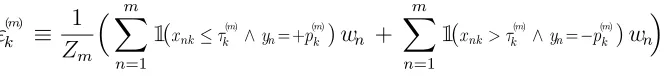
data), we can expand the weighted classification error (Eq. 3.1) as:

εk = 1

Z

_XN

n=1

1(xnk≤τ ∧yn=+p)wn + N

X

n=1

1(xnk> τ ∧yn=−p)wn

In practice, this error is minimized by findingk∗_{; the best single feature of them all:}

(p∗, τ∗, k∗) _≡ arg min

p,τ,kεk ε ∗

≡ εk∗

In current implementations of boosting [31], feature values can first be quantized intoB bins by linearly distributing them in[1, B](outer bins corresponding to the min/max, or to a fixed number of standard deviations from the mean), or by any other quantization method. Not surprisingly, using too few bins reduces threshold precision and hence overall performance. We find thatB = 256is large enough to incur no loss in practice.

Determining the optimal thresholdτ∗ _{requires accumulating each sample’s weight} into discrete bins corresponding to that sample’s feature valuexnk. This procedure turns out to still be quite costly: for each of thedfeatures, the weights of each of the N samples have to be accumulated in bins, causing the training of a single stump to be anO(d_×N)operation; the very bottleneck of training boosted decision trees.

In the following sections, we examine the training process in greater detail and develop an intuition for how we can reduce computational costs.

Progressively Increasing Subsets

Let us assume that at the start of each boosting iteration, the data samples are sorted in order of decreasing weight, i.e: r < m _⇒ wr ≥ wm. Consequently, we define

Zm, the mass of theheaviestsubset ofmdata points:

Zm ≡

m

X

n=1

wn [note:ZN ≡ Z]

Clearly, Zm is greater or equal to the sum of any m other sample weights. As we increase m, them-subset includes more samples, and accordingly, its massZm increases (although at a diminishing rate).

Since training time is dependent on the number of samples and not on their cumula-tive weight, we should be able to leverage this fact and train using only a subset of the data. The more non-uniform the weight distribution, the more we can leverage; boosting is an ideal situation where few samples account for most of the weight.

0.3% 1% 3% 10% 30% 100%

0% 20% 40% 60% 80% 100%

Relative Subset Size (m/N)

R

el

a

ti

v

e

S

u

b

se

t

M

a

ss

(

Zm

/Z

)

AdaBoost LogitBoost L

2 Boost

Figure 3.2: Progressively increasing m-subset mass using different variants of boosting. Relative subset mass Zm/Z exceeds 90% after only m/N ≈ 7% for AdaBoost andm/N _≈20%forL2Boost.

The same observation was made by [20], giving rise to the idea ofweight-trimming, which proceeds as follows. At the start of each boosting iteration, samples are sorted in order of weight (from largest to smallest). For that iteration, only the sam-ples belonging to the smallestm-subset such thatZm/Z ≥ ηare used for training (where η is some predefined threshold); all the other samples are temporarily ig-nored – ortrimmed. Friedman et al. claimed this to“dramatically reduce computa-tion for boosted models without sacrificing accuracy.”In particular, they prescribed η= 90% to 99%“typically”, but they left open the question of how to chooseηfrom the statistics of the data [20].

Their work raises an interesting question: Is there a principled way to determine (and train on only) the smallest subset after which including more samples does not

alter the final stump? Indeed, we prove that a relatively smallm-subset contains enough information to set the optimal stump; thereby saving a lot of computation.

Preliminary Errors

Definition: given a featurekand anm-subset, thebest preliminary errorε(m)

ε(_km) _≡ 1 Zm

_Xm

n=1

1(xnk≤τ

(m)

k ∧yn=+p

(m)

k )wn +

m

X

n=1

1(xnk> τ

(m)

k ∧yn=−p

(m)

k)wn

[wherep(m_k) andτ_k(m) are optimal preliminary parameters]

The emphasis on preliminary indicates that the subset does not contain all data points, i.e:m < N, and the emphasis onbestindicates that no choice of polarityp or thresholdτ can lead to a lower preliminary error using that feature.

As described above, given a feature k, a stump is trained by accumulating sample weights into bins. We can view this as a progression; initially, only a few samples are binned, and as training continues, more and more samples are accounted for. As revealed by the smoothness of the traces,ε(km) may be computed incrementally.

60% 70% 80% 90% 100%

30% 35% 40% 45% 50%

Relative Subset MassZm/Z

P

re

li

m

in

a

ry

E

rr

o

r

ε

(

m

)

6.5% 9.3% 10.7% 29.8% 100%

Relative Subset Sizem/N

Figure 3.3: Traces of the best preliminary errors over increasing Zm/Z. Each curve corresponds to a different feature k. The dashed orange curve corresponds to a feature that turns out to be misleading (i.e. its final error drastically worsens when all the sample weights are accumulated). The thick green curve corresponds to the optimal feature; note that it is among the best performing features even when training with relatively few samples.

Figure 3.3 shows the best preliminary error for each of the features in a typical experiment. By examining Figure 3.3, we can make four observations:

2. Feature errors increasingly stabilize asm _→N

3. The best performing features at smallerm-subsets (i.e. Zm/Z < 80%) can end up performing quite poorly once all of the weights are accumulated (dashed orange curve)

4. The optimal feature is among the best features for smallerm-subsets as well (solid green curve)

From the full training run shown in Figure 3.3, we note (in retrospect) that using an m-subset with m/N _≈ 0.2would suffice in determining the optimal feature. But how can we knowa prioriwhichmis good enough?

60% 70% 80% 90% 100%

0% 20% 40% 60% 80% 100%

Relative Subset MassZm/Z

P

ro

b

a

b

il

it

y

optimum among: preliminary top 1 preliminary top 10 preliminary top 10%

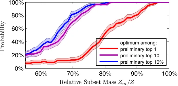
Figure 3.4: Probability that the optimal feature is among the K top-performing features. The red curve corresponds toK_{= 1}, the purple toK _{= 10}, and the blue toK= 1%of all features. Note the knee-point aroundZm/Z ≈ 75%at which the optimal feature is among the 10 preliminary-best features over 95% of the time.

Averaging over many training iterations, in Figure 3.4, we plot the probability that the optimal feature is among the top-performing features when trained on only an m-subset of the data. This gives us an idea as to how small m can be while still correctly predicting the optimal feature.

3.4 Pruning Underachieving Features

Figure 3.4 suggests that the optimal feature can often be estimated at a fraction of the computational cost using the following heuristic:

Faulty Stump Training

1. Train each feature only with samples in them-subset whereZm/Z ≈75%. 2. Prune all but the 10 best performing features.

3. For each of un-pruned feature, complete training on the entire data set. 4. Finally, report the best performing feature (and corresponding parameters).

This heuristic does not guarantee to return the optimal feature, since premature pruning can occur in step 2. However, if we were somehow able to bound the error, we would be able to prune features that would provably underachieve (i.e. would no longer have any chance of being optimal in the end).

Definition: a featurek is denotedunderachieving if it is guaranteed to perform worse than the best-so-far featurek◦ _{on the entire training data.}

Proposition 3.2: for a featurek, the following bound holds (proof given in Sec-tion 3.4): given two subsets (where one is larger than the other), the product of subset mass and preliminary error is always greater for the larger subset:

r _≤m _⇒ Zrε

(r)

k ≤ Zmε

(m)

k (3.2)

Let us assume that the best-so-far errorε◦ _{has been determined over a few of the} features (and the parameters that led to this error have been stored). Hence, this is an upper-bound for the error of the stump currently being trained. For the next feature in the queue, even after a smaller (m < N)-subset, then:

Zmε

(m)

k ≥ Z ε ◦

⇒ Z εk ≥ Z ε◦ ⇒ εk ≥ ε◦

Therefore, if: Zmε

(m)

k ≥ Z ε◦ then feature k is underachievingand can safely be pruned. Note that the lower the best-so-far error ε◦_{, the harsher the bound;} conse-quently, it is desirable to train a relatively low-error feature early on.

Quick Stump Training

1. Train each feature only using data in arelatively smallm-subset. 2. Sort the features based on their preliminary errors (from best to worst). 3. Continue training one feature at a time on progressively larger subsets,

updatingε(km) after accumulating the samples in each subset.

•if it is underachieving, prune immediately. •if it trains to completion, save it as best-so-far.

4. Finally, report the best performing feature (and corresponding parameters).

Subset Scheduling

Deciding which schedule ofm-subsets to use is a subtlety that requires further ex-planation. Although this choice does not effect the optimality of the trained stump, it may effect speedup. If the first“relatively small”m-subset (as prescribed in step 1) is too small, we may lose out on low-error features leading to less-harsh pruning. If it is too large, we may be doing unnecessary computation. Furthermore, since the calculation of preliminary error does incur some (albeit, low) computational cost, it is impractical to use everymwhen training on progressively larger subsets.

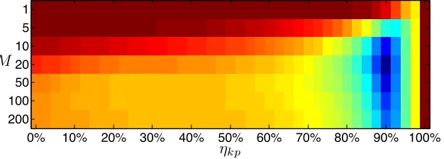
To address this, we implement a simple schedule: The firstm-subset is determined by the parameterηkpsuch thatZm/Z ≈ηkp. M following subsets are equally spaced

out between ηkp and1. Figure 3.5 shows a parameter sweep overηkp andM, from

which we fixηkp= 90%andM = 20and use this setting for all of our experiments.

ηkp M

0% 10% 20% 30% 40% 50% 60% 70% 80% 90% 100%

1

5

10

20

50

100

200

Figure 3.5: Computational cost of training boosted trees over a range of ηkp and

M, averaged over several types of runs (with varying numbers and depths of trees). Red corresponds to higher cost, blue to lower cost. All final classifiers are identical. Standard training corresponds toηkp= 100%, resulting in the highest computational

cost. The lowest computational cost is achieved atηkp= 90%andM = 20.

underachiev-ing features, a lot of computation is saved. We now outline the full boostunderachiev-ing proce-dure using our quick training method:

Quickly Boosting Decision Trees

1. Initialize weights(sorted in decreasing order).

2. Train decision treeft(one node at a time) usingQuick Stump Training. 3. Perform standard boosting steps:

(a) determine optimalαt(e.g. closed-form optimum or using line-search).

(b) update sample weights given the misclassification error offt,

according to the specific variant of boosting being used.

(c) if more boosting iterations are needed, sort sample weights in decreasing

order, increment iteration numbert; goto step 2.

We note that sorting the weights in step 3(c) above is anO(N)operation. Given an initially sorted set, boosting updates the sample weights based on whether the sam-ples were correctly classified or not. All correctly classified samsam-ples are weighted down, but they maintain their respective ordering. Similarly, all misclassified sam-ples are weighted up, also maintaining their respective ordering. Finally, these two sorted lists are merged inO(N).

We now give a proof for the bound that our method is based on, and in the following section, we demonstrate its effectiveness in practice.

Proof of Proposition 3.2

As previously defined,ε(_km) is the preliminary weighted classification error computed using the featurekon samples in them-subset; thus:

Zmε

(m)

k = m

X

n=1

1(xnk≤τ

(m)

k ∧yn=+p

(m)

k)wn +

m

X

n=1

1(xnk> τ

(m)

k ∧yn=−p

(m)

k )wn

Proposition 3.2: r_≤m _⇒ Zrε

(r)

k ≤ Zmε

(m)

k

Proof: ε(_kr) is the best achievable preliminary error on ther-subset (and correspond-ingly,(p(kr), τ

(r)

k )are the best preliminary parameters); therefore:

Zrε

(r)

k ≤ r

X

n=1

1(xnk≤τ ∧yn=+p)wn + r

X

n=1

Hence, switching the optimal parameters(p(rk), τ

(r)

k )for potentially sub-optimal ones (p(m_k), τ_k(m))(note the subtle change in indices on the right side of the inequality):

Zrε

(r)

k ≤ r

X

n=1

1(xnk≤τ

(m)

k ∧yn=+p

(m)

k)wn +

r

X

n=1

1(xnk> τ

(m)

k ∧yn=−p

(m)

k )wn

The resulting sum can only increase when summing over a larger subset (m_≥r):

Zrε

(r)

k ≤ m

X

n=1

1(xnk≤τ

(m)

k ∧yn=+p

(m)

k)wn +

m

X

n=1

1(xnk> τ

(m)

k ∧yn=−p

(m)

k )wn

But the right-hand side of the inequality is equivalent toZmε

(m)

k ; thus:

r _≤m _⇒ Zrε

(r)

k ≤ Zmε

(m)

k

Q.E.D.

For similar proofs using information gain, Gini impurity, or variance minimization as split criteria, refer to Appendix 7.2.

3.5 Experiments

In the previous section, we proposed an efficient stump training algorithm and showed that it has a lower expected computational cost than the traditional method. In this section, we describe experiments that are designed to assess whether the method is practical and whether it delivers significant training speedup. We train and test on three real-world datasets and empirically compare the speedups.

Datasets

We trained AdaBoosted ensembles of shallow decision trees of various depths on the following three datasets:

1. CMU-MIT Faces dataset [29]; 8.5_·103 _{training and 4.0·10}3 _{test samples,}

4.3_·103 _{features used are the result of convolutions with Haar-like wavelets}

[33], using 2000 stumps as in [33].

2. INRIA Pedestrian dataset [10]; 1.7_·104 _{training and 1.1·10}4 _{test samples,}

5.1_·103 _{features used are Integral Channel Features [13]. The classifier has}

4000 depth-2 trees as in [13].

3. MNIST Digits [23];6.0_·104_{training and1.0·10}4_{test samples,7.8·10}2_features

(1) (2) T ra in in g L o ss (a ) 109 1010

10−12

10−10

10−8

10−6

10−4

10−2

AdaBoost

Weight−Trimming 99%

Weight−Trimming 90%

LazyBoost 90% LazyBoost 50% StochasticBoost 50% T es t E rr o r (a ) 108 109 1010 10−4

10−3 10−2

AdaBoost Weight−Trimming 99% Weight−Trimming 90% LazyBoost 90% LazyBoost 50% StochasticBoost 50% T ra in in g L o ss (b ) 1010 1011

10−70

10−60 10−50

10−40

10−30

10−20

10−10

AdaBoost Weight−Trimming 99% Weight−Trimming 90% LazyBoost 90% LazyBoost 50% StochasticBoost 50% T es t E rr o r (b ) 109 1010 1011 10−3

10−2

AdaBoost Weight−Trimming 99% Weight−Trimming 90% LazyBoost 90% LazyBoost 50% StochasticBoost 50% T ra in in g L o ss (c )

109 1010

10−50

10−40

10−30

10−20

10−10

AdaBoost Weight−Trimming 99% Weight−Trimming 90% LazyBoost 90% LazyBoost 50% StochasticBoost 50% T es t E rr o r (c ) 108 109 1010

10−2

AdaBoost

Weight−Trimming 99%

Weight−Trimming 90%

LazyBoost 90% LazyBoost 50% StochasticBoost 50%

Computational Cost Computational Cost

Figure 3.6: Computational cost versus training loss (left plots) and versus test error (right plots) for the various heuristics on three datasets: (a1,2) CMU-MIT

Faces, (b1,2) INRIA Pedestrians, and (c1,2) MNIST Digits [see text for details].

Dashed lines correspond to the “quick” versions of the heuristics (using our pro-posed method) and solid lines correspond to the original heuristics. Test error is defined as the area over the ROC curve.

Comparisons

Quick Boosting can be used in conjunction with all previously mentioned heuristics to provide further gains in training speed. We report all computational costs in units proportional to Flops, since running time (in seconds) is dependent on compiler optimizations which are beyond the scope of this work.

We comparevanilla(no heuristics) AdaBoost, Weight-Trimming withη= 90% and 99% [see Sec. 3.3], LazyBoost 90% and 50% (only 90% or 50% randomly selected features are used to train each weak learner), and StochasticBoost (only a 50% random subset of the samples are used to train each weak learner). To these six heuristics, we apply our method to produce six “quick” versions.

We further note that our goal in these experiments is not to tweak and enhance the performance of the classifiers, but to compare the performance of the heuristics with and without our proposed method.

Results and Discussion

From Figure 3.6, we make several observations. “Quick” versions require less com-putational costs (and produce identical classifiers) as theirslowcounterparts. From the training loss plots (5a1,5b1,5c1), we gauge the speed-up offered by our method,

often around an order of magnitude. Quick-LazyBoost-50% and Quick-Stochastic-Boost-50% are the least computationally-intensive heuristics, andvanillaAdaBoost always achieves the smallest training loss and attains the lowest test error in two of the three datasets.

The motivation behind this work was to speed up training such that (i) for a fixed computational budget, the best possible classifier could be trained, and (ii) given a desired performance, a classifier could be trained with the least computational cost.

For each dataset, we find the lowest-cost heuristic and set that computational cost as our budget. We then boost as many weak learners as our budget permits for each of the heuristics (with and without our method) and compare the test errors achieved, plotting the relative gains in Figure 3.7. For most of the heuristics, there is a two to eight-fold reduction in test error, whereas for weight-trimming, we see less of a benefit. In fact, for the second dataset, Weight-Trimming-90% runs at the same cost with and without our speedup.

Conversely, in Figure 3.8, we compare how much less computation is required to achieve the best test error rate by using our method for each heuristic. Most heuris-tics see an eight to sixteen-fold reduction in computational cost, whereas for weight-trimming, there is still a speedup, albeit only between one and two-fold.