On the calculation of normals in free-surface flow problems

White Rose Research Online URL for this paper:

http://eprints.whiterose.ac.uk/1738/

Article:

Walkley, M.A., Gaskell, P.H., Jimack, P.K. et al. (3 more authors) (2004) On the calculation

of normals in free-surface flow problems. Communications in Numerical Methods in

Engineering, 20 (5). pp. 343-351. ISSN 1099-0887

DOI:10.1002/cnm.677

Reuse

See Attached

Takedown

If you consider content in White Rose Research Online to be in breach of UK law, please notify us by

White Rose Consortium ePrints Repository

http://eprints.whiterose.ac.uk/

This is an author produced version of a paper published in Communications in

Numerical Methods in Engineering.

White Rose Repository URL for this paper:

http://eprints.whiterose.ac.uk/1738/

Published paper

Walkley, M.A., Gaskell, P.H., Jimack, P.K., Kelmanson, M.A., Summers, J.L. and

Wilson, M.C.T. (2004) On the calculation of normals in free-surface flow

problems. Communications in Numerical Methods in Engineering, 20 (5).

pp. 343-351.

On the calculation of normals in free-surface flow problems

M.A. Walkley

, P.H. Gaskell

, P.K. Jimack

, M.A. Kelmanson

,

J.L. Summers

and M.C.T. Wilson

1_{School of Computing, University of Leeds, Leeds, LS2 9JT, UK} 2_{School of Mechanical Engineering, University of Leeds, Leeds, LS2 9JT, UK} 3_{Department of Applied Mathematics, University of Leeds, Leeds, LS2 9JT, UK}

SUMMARY

The use of boundary-conforming finite-element methods is considered for the solution of

surface-tension-dominated free-surface flow problems in three dimensions. This class of method is based upon the use of a

moving mesh whose velocity is driven by the motion of the free surface, which is in turn determined via a

kinematic boundary condition for the normal velocity. The significance of the method used to compute the normal

direction at the finite-element node points for a C0piecewise-polynomial free surface is investigated. In particular,

it is demonstrated that the concept of mass-consistent normals on an isoparametric quadratic tetrahedral mesh

is flawed. In this case an alternative, purely geometric, normal is shown to lead to a far more robust numerical

algorithm. Copyright c­2003 John Wiley & Sons, Ltd.

KEY WORDS: Finite element method; Free surface flow; Surface tension; Normals

1. INTRODUCTION

Free-surface flow problems are of great importance in the modelling of a wide range of physical

phenomena, from phase-change problems [1, 2] through to coating flows [3, 4], sintering [5, 6] or the

Correspondence to: M.A. Walkley, School of Computing, University of Leeds, Leeds, LS2 9JT, UK.

Email:[email protected]

spreading of viscous fluids [7, 8]. In two dimensions, computational fluid dynamics (CFD) techniques

for solving time-dependent free-surface problems are becoming well established [6, 9, 10] and, in three

dimensions, there has been a significant amount of important recent research [2, 11, 12, 13]. One of the

most popular classes of methods in both two and three dimensions is based upon the use of

boundary-conforming moving/adapting meshes, as in the arbitrary Lagrangian-Eulerian (ALE) finite element

method. Other techniques include Eulerian algorithms such as the volume-of-fluid method [14, 15]. In

such methods a larger domain is required than the region occupied by a single fluid and the interface

is reconstructed in some manner, usually through the use of a characteristic or auxiliary function. In

order to maintain accuracy with this approach, considerable local mesh refinement is required to track

the free surface. Conversely, purely Lagrangian algorithms have also been developed, such as those

described in [16, 17]. These too have the potential to be highly accurate but often at the expense of

frequent remeshing. In this paper, however, attention is restricted to ALE algorithms in which the mesh

conforms to the dynamic free surface at all times.

One of the main advantages of boundary-conforming ALE algorithms is their potential to represent

the moving free surface to a very high accuracy. Surface-tension effects couple the geometry of the free

surface to its motion, which in turn induces flow effects in the bulk fluid. Hence the ability to accurately

model the geometry and the kinematics of the free surface is generally of great importance. Usually,

the representation of the surface takes the form of a C0_{piecewise polynomial whose accuracy can be}

maintained through the use of local mesh refinement as the solution—and therefore the boundary—

evolves. A significant amount of work has been undertaken in both two and three dimensions using

this approach. Examples include, but are not limited to, the work of Cairncross et al. [11], Lynch et al.

[1, 18], Peterson et al. [10, 19], Soulaimani and Saad [12], and Zhou and Derby [13].

In the present paper, a three-dimensional ALE algorithm is presented based on standard

isoparametric tetrahedral Taylor-Hood finite elements. This is a generalization of the two-dimensional

work of [10, 19]. It is demonstrated that, in the presence of a kinematic boundary condition which

stipulates the normal motion of the free surface, the manner in which the normal to the

piecewise-polynomial boundary is calculated is of critical importance. In particular, an observation is presented

that the use of so-called mass-consistent normals [18, 20] is no longer valid for this finite element

discretisation in three dimensions, despite being the de facto implementation in the two-dimensional

2. OVERVIEW OF THE SOLUTION ALGORITHM

The precise ALE algorithm used for this work is an extension of the two-dimensional work in [10]

and therefore only a brief overview is provided. It is emphasized, however, that the conclusions of this

work are neither specific nor restricted to the precise ALE implementation used herein.

The following non-dimensional form of the incompressible Navier-Stokes equations is considered;

Re

∂u

∂t

u∇u

∇St f (1)

∇u 0 (2)

Here u is velocity, pI∇u∇u

T _{is the stress tensor, p is pressure, I is the identity tensor,}

Re the Reynolds number, St the Stokes number and f the exterior force. At a solid boundary, the

no-slip boundary condition is applied and, at a free surface the following kinematic condition and stress

condition are applied:

nu x˙

f s 0 (3)

n npext

1

Ca

∇_Sn

n (4)

In (3) n represents the outward normal to the free surface whose location is given by x_{f s}, u represents

the fluid velocity at a point on the free surface and the dot above a variable denotes its time derivative.

In (4) pext is the external pressure, which may be taken as zero for simplicity,∇_SI nn∇is the surface gradient operator and Ca is the capillary number which is inversely proportional to surface

tension (which in the present work is assumed constant over the entire free surface).

The problem is simplified by considering Stokes flows only, for which Re is zero, in the absence of

gravity, so that f vanishes. Equations (1) and (2) are discretized using an isoparametric Taylor-Hood

finite-element method with quadratic velocities and linear pressures on an unstructured tetrahedral

mesh, which is known to be stable [20]. On the piecewise-quadratic free surface, the natural boundary

condition (4) is imposed weakly, followed by application of the surface divergence theorem. Having

obtained an instantaneous velocity field, the kinematic boundary condition (3) is used to determine

the instantaneous normal motion on the free surface; note that this step depends critically upon the

definition chosen for the normal direction along free-surface edges and at free-surface nodes.

The position of the free surface is updated explicitly using the normal velocity just computed. This

requires updating at the end of each time step. To achieve this a linear elasticity model, similar to that

described in [11], is used. Effectively, the nodes in the mesh are treated as points in a linear elastic

material which is deformed by applying a displacement that is equal to the displacement in the free

surface over the time step. This uniquely determines the displacement of each point in the mesh in a

manner that prevents tangling, at least for moderate free-surface motions. Having updated both the free

surface and the mesh, the solution of (1) and (2) may now be computed to obtain the instantaneous

velocity field at the start of the next time step.

As indicated in the introduction, there is an important issue associated with the kinematic boundary

condition (3) since, for a typical finite-element solution, n is not uniquely defined in three dimensions

at node points and element edges on the free surface. Numerical techniques such as that described

above, however, seek to apply (3) at the nodes on this surface, either explicitly or implicitly, in order to

update the boundary location over a time step.

3. COMPUTATION OF THE BOUNDARY NORMALS

There are a number of possible ways in which one may interpret (3) at a finite-element node on

the free surface. In the numerical investigations described below, two different choices of normal

direction are considered. In particular, the standard mass-consistent normals, used successfully in the

two-dimensional algorithm, are shown not to generalize to three-dimensional algorithms of the form

described in Section 2.

Mass-consistent normals

In [20], results of Engelman et al. [21] are described in which the unit normal at node j, n_j say, is

derived from the discrete weak continuity equation for incompressible flow. After some algebra this

yields the expression

n_j

Ê

Γnφjds

Ê

Γnφjds

(5)

whereΓis the free surface andφ_jis the finite-element velocity basis function at node j. Note that this

expression for the normal is also used by Lynch and Gray [18], although they do not derive it from

the view point of mass conservation. In [20], (5) is referred to as the mass-consistent normal.

by several authors including the two-dimensional version of the algorithm described in Section 2 [10].

An important observation when seeking to employ (5) at a vertex, j say, is that the expression

takes the form of a weighted average normal, with the vertex basis function,φ_j, acting as the weight.

For three-dimensional quadratic tetrahedral elements this weight is non-positive, and in particular the

vertex basis function,φ_j, has the property that

Γ

φ_jds 0 (6)

This is a particularly undesirable property for the computation of the mass-consistent normal. For

example, if the mass consistent normal is computed on a plane surface, where the normal is constant,

the result will be the zero vector if (5) is used. Even on a curved surface on which the normal varies

smoothly on an element, with jump discontinuities between the elements, the property (6) ensures that

the quality of the normal computed by (5) will be very poor, being greatly affected by cancellation, and

often not at all representative of the local surface geometry. Note that the edge nodes of the quadratic

tetrahedral elements are unaffected since the basis functions associated with these nodes are always

positive and the mass-consistent normal can be computed reliably at these points.

In the two-dimensional case, when isoparametric quadratic triangular elements are used, the problem

does not manifest itself. The vertex basis functions,φ_j, are again non-positive but in this case satisfy

Γ φ_jds

1

6 0 (7)

As outlined below, this is sufficient to ensure that problems do not occur in two dimensions.

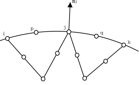
Considering a one-dimensional piecewise-quadratic segment of the finite-element domain boundary,

depicted in Figure 1, a precise form for the mass-consistent normal (5) can be derived by substitution

of the standard quadratic basis functions. The numerator of the mass consistent normal (5) at the vertex,

n_j, can be written as

n_j 1 6

y

k yi 4yq yp x

k xi4xp xq

(8)

Note that if, for example, y

k yi4yq ypthe x-component of the normal can be made zero,

with a similar possibility for the y-component. However, the distortion to the element implied by these

equalities occurring simultaneously would be such that the Jacobian of the isoparametric mapping

becomes singular. Furthermore, previous work in two dimensions [10, 19] avoids such potential

difficulties by automatically maintaining the position of the edge nodes at the centre of the quadratic

isoparametric mapping does not become near-to singular, but has the additional effect of ensuring that

the mass-consistent normals work as designed in two dimensions.

Arithmetic-average normals

An alternative expression for the normal to a finite-element free surface node may be obtained from

purely geometric considerations, i.e. by taking the average normal direction from elements sharing that

node. At the general node j, this yields the expression

n_j

1 Nj

∑Nj

k1

nx

j

Ω_jk

1 Nj

∑Nj

k1

nx

j

Ω_jk

(9)

Here x_j is the location of node j, Nj is the number of free-surface elements sharing node j,

Ω

j1Ω

jNj is the set of these elements, and nx

j

Ω is the limit of nxas x approaches

x_j from within the free surface of elementΩ. This approach of calculating an arithmetic average of

the normal on neighbouring elements has been reported in the three-dimensional work of [11], which

uses linear hexahedral elements, though they do not comment on alternative methods for computing

the normal.

It is demonstrated in the following section that use of the arithmetic-average normal allows robust

computation for some typical three-dimensional free-surface flows and mass is conserved with a high

degree of accuracy. The weakness of the mass-consistent approach for quadratic tetrahedral elements

is further highlighted, despite its successful use for two-dimensional problems.

4. NUMERICAL RESULTS

Results are presented for the solution of two simple model problems in three dimensions using the

algorithm of Section 2. The first problem involves a large induced tangential velocity field on the free

surface, with the normal motion of the surface expected to be small. The second problem comprises a

large deformation of the fluid surface, and hence significant movement of the free surface as it recovers

to its equilibrium state. The spatial domain considered for both problems consists of a thick layer

of fluid covering a sphere of unit radius. The numerical model thus consists of a solid-wall interior

boundary and a free-surface exterior boundary surrounding the fluid. This domain is discretized using

719 elements and 1433 nodes. A two-dimensional example is also presented, analogous to the second

three-dimensional example, to illustrate the successful use of the mass-consistent normals in this case.

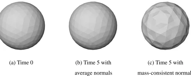
4.1. A rotating spherical core

Fluid is initially distributed in a uniform spherical shell about a central spherical solid core which is

rotating with unit angular velocity about the z-axis. This induces a relatively large tangential velocity

on the free surface, compared to the normal component. In the absence of gravity and inertial terms no

significant normal motion of the free surface is expected. Problems with large tangential velocities are

not unrealistic for this type of fluid model, occurring, for example, in studies of the supported load on

a rotating cylinder [19].

Figure 2(a)-(b) shows the free surface shape produced when using the arithmetic-average normals.

As can be seen, the surface varies imperceptibly from its initial state, since no normal motion is

generated by the tangential velocity field. Although the results with the arithmetic-average normals

show a steady loss of mass over time, the actual amount is small in relative terms, being approximately

10 2% after 104time steps (a real time of t=10, corresponding to 5π sphere rotations). Given that

the mesh employs only 719 elements, it should be borne in mind that even this small loss of mass

may be reduced further by using a finer grid. Figure 2(c) shows the distinctly non-physical nature of

the surface produced when mass-consistent normals are used. An equilibrium position is reached that

bears no relation to the expected physical result since the computed surface normals are not initially

perpendicular to the tangential velocity field. Note, however, that mass is conserved in this case to

within 10 3% over the same simulation time.

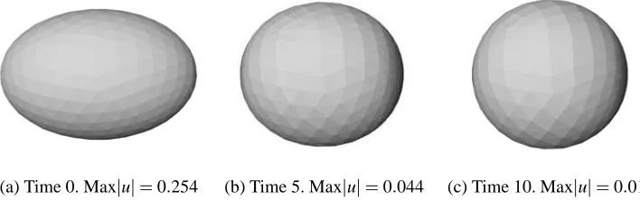
4.2. Perturbed free surface

In this case a problem is considered in which a large normal motion of the fluid free surface is expected.

The free surface of the fluid is stretched along the x-axis by a factor 15 into an initially elliptical shape.

In the absence of gravity, surface tension will tend to draw the fluid back into a sphere about the inner

core.

Using the arithmetic-average normals the solution is computed for 104 time steps (a real time of

t=10) and it evolves smoothly towards the expected spherical shape, as depicted in Figure 3. The

volume change during the simulation, even after 104time steps, is only 510

3_{% of the total volume.}

completely.

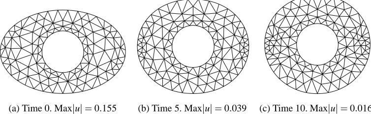
4.3. Comparison with two-dimensional simulations

Results from the two-dimensional algorithm have been presented elsewhere [10, 19]. Here a single

example is shown employing mass-consistent normals, illustrating their successful use in this case.

An annular layer of fluid, surrounding a solid circular internal boundary, is initially stretched into an

elliptical shape; in the absence of gravity it returns to the circular equilibrium position under the action

of surface tension. Figures 4(a)-(c) show the evolution of the free-surface shape and the maximum

velocity magnitude computed on the free surface. During 104time steps (a real time of t=10) of the

simulation on this relatively coarse mesh mass is conserved to within 210

4_{%, emphasising the utility}

of the mass-consistent normals in this two-dimensional case.

5. CONCLUSIONS

Surface tension is the dominating force for a large class of physical problems, and the accuracy of

computational models for such problems therefore depends critically on the accurate representation of

the curvature of the fluid free surface, which in turn is used to determine the motion of the free surface.

The mass-consistent normal is derived from the viewpoint of mass conservation and as such appears

to work well for many problems. As shown in Section 3 however there is a serious flaw in applying

this method to the standard Taylor-Hood tetrahedral finite element method in three dimensions, and

while the method will generally work in the two-dimensional case it is necessary to ensure that the

edge nodes are constrained to lie close to the midpoint of the edges. The numerical results in Section 4

corroborate these observations.

The arithmetic-average normals described in Section 3 do not have any implicit mass-conservation

properties but are accurate in the sense that they are derived from the geometry of the free surface. In

practice they always provide a smooth evolution of the free surface and flow field. The results show

that, with this choice, the volume of the fluid decreases over time, but the rate of decrease is relatively

small, even when using the quite coarse meshes in the examples above. Hence for tetrahedral

Taylor-Hood elements these normals are to be preferred.

The authors wish to thank an anonymous referee for many helpful comments on the manuscript.

REFERENCES

1. Lynch DR, O’Neill K. Continuously deforming finite elements for the solution of parabolic problems, with and without

phase change. Int. J. Numer. Meth. Fluids, 1981; 17:81–96.

2. Schmidt A. Computation of three dimensional dendrites with finite elements. J. Comput. Phys., 1996; 125:293–312.

3. Gaskell PH, Savage MD, Summers JL, Thompson HM. Modelling and analysis of meniscus roll coating. J. Fluid Mech.,

1995; 298:113–137.

4. Kistler SF, Schweizer PM (eds). Liquid Film Coating. Chapman Hall, 1997.

5. Kuiken HK. Viscous sintering: The surface-tension-driven flow of a liquid form under the influence of curvature gradients

at its surface. J. Fluid Mech., 1990; 214:503–515.

6. van de Vorst GAL, Mattheij RMM, Kuiken HK. A boundary element solution for two-dimensional viscous sintering. J.

Comput. Phys., 1992; 100:50–63.

7. Marar OK, Troians SM. The development of transient fingering patterns during the spreading of surfactant coated films.

Phys. Of Fluids, 1999; 11:3232–3246.

8. Moriarty JA, Schwartz LW, Tuck EO. Unsteady spreading of thin liquid films with small surface tension. Physics of

Fluids, 1991; 3:733–751.

9. Mashayek F, Ashgriz N. A spine-flux method for simulating free surface flows. J. Comput. Phys., 1995; 122:367–399.

10. Peterson RC, Jimack PK, Kelmanson MA. The solution of two-dimensional free-surface problems using automatic mesh

generation. Int. J. Numer. Meth. Fluids, 1999; 31:937–960.

11. Baer TA, Cairncross RA, Schunk PR, Rao RR, Sackinger PA. A finite element method for free-surface flows of

incompressible fluids in three dimensions. Part I. Boundary-fitted mesh motion. Int. J. Numer. Meth. Fluids, 2000; 33:375–

403.

12. Soulaimani A, Saad Y. An arbitrary Lagrangian–Eulerian finite element method for solving three-dimensional free surface

flows. Comp. Meth. Appl. Mech. Eng., 1998; 162:79–106.

13. Zhou H, Derby JJ. An assessment of a parallel, finite element method for three-dimensional, moving-boundary flows

driven by capillarity for simulation of viscous sintering. Int. J. Numer. Meth. Fluids, 2001; 36:841–865.

14. Cerne G, Petelin S, Tiselj I. Numerical errors of the volume-of-fluid interface tracking algorithm. Int. J. Numer. Meth.

Fluids, 2002; 38:329–350.

15. Hirt CW, Nichols BD. Volume of fluids methods for the dynamics of free boundaries. J. Comput. Phys., 1981; 39:201–225.

16. Muttin F, Coupez T, Bellet M, Chenot JL. Lagrangian finite-element analysis of time-dependent free-surface flow using

an automatic remeshing technique – application to metal casting. Int. J. Numer. Meth. Eng., 1993; 36:2001-2015.

17. Ramaswamy B, Kawahara M. Lagrangian finite-element analysis applied to viscous free-surface fluid flow. Int. J. Numer.

Meth. Fluids, 1987; 7:953–984.

18. Lynch DR, Gray WG. Finite element simulation of flow in deforming regions. J. Comput. Phys., 1980; 36:135–153.

19. Peterson RC, Jimack PK, Kelmanson MA. On the stability of viscous free-surface flow supported by a rotating cylinder.

Proc. R. Soc. Lond. A, 2001; 457:1427–1445.

21. Engelman MS, Sani RL, Gresho PM. The implementation of normal and/or tangential boundary conditions in finite element

codes for incompressible fluid flow. Int. J. Numer. Meth. Fluids, 1982; 2:225–238.

22. Sch ¨oberl J. NETGEN - An advancing front 2D/3D-mesh generator based on abstract rules. Comput. Visual. Sci, 1997;

i

j

k nj

p

q

(a) Time 0 (b) Time 5 with (c) Time 5 with

average normals mass-consistent normals

(a) Time 0. Maxu0254 (b) Time 5. Maxu0044 (c) Time 10. Maxu0013

(a) Time 0. Maxu0155 (b) Time 5. Maxu0039 (c) Time 10. Maxu0016