C
2011. The American Astronomical Society. All rights reserved. Printed in the U.S.A.
KEPLER-14b: A MASSIVE HOT JUPITER TRANSITING AN F STAR IN A CLOSE VISUAL BINARY
Lars A. Buchhave1,2, David W. Latham3, Joshua A. Carter3,26, Jean-Michel D´esert3, Guillermo Torres3, Elisabeth R. Adams3, Stephen T. Bryson4, David B. Charbonneau3, David R. Ciardi5, Craig Kulesa6, Andrea K. Dupree3, Debra A. Fischer7, Fran¸cois Fressin3, Thomas N. Gautier III8, Ronald L. Gilliland9, Steve B. Howell4, Howard Isaacson10, Jon M. Jenkins11, Geoffrey W. Marcy10, Donald W. McCarthy12, Jason F. Rowe11, Natalie M. Batalha13, William J. Borucki4, Timothy M. Brown14, Douglas A. Caldwell11,
Jessie L. Christiansen11, William D. Cochran15, Drake Deming16, Edward W. Dunham17, Mark Everett18,
Eric B. Ford19, Jonathan J. Fortney20, John C. Geary3, Forrest R. Girouard21, Michael R. Haas4,
Matthew J. Holman3, Elliott Horch22, Todd C. Klaus21, Heather A. Knutson10, David G. Koch4,
Jeffrey Kolodziejczak23, Jack J. Lissauer4, Pavel Machalek11, Fergal Mullally11, Martin D. Still24,
Samuel N. Quinn3, Sara Seager25, Susan E. Thompson11, and Jeffrey Van Cleve11 1Niels Bohr Institute, University of Copenhagen, DK-2100 Copenhagen, Denmark
2Centre for Star and Planet Formation, Natural History Museum of Denmark, University of Copenhagen, DK-1350 Copenhagen, Denmark 3Harvard-Smithsonian Center for Astrophysics, Cambridge, MA 02138, USA
4NASA Ames Research Center, Moffett Field, CA 94035, USA
5NASA Exoplanet Science Institute/California Institute of Technology, Pasadena, CA 91109, USA 6Lunar and Planetary Laboratory, University of Arizona, Tucson, AZ 85721, USA
7Department of Astronomy, Yale University, New Haven, CT 06511, USA 8Jet Propulsion Laboratory/California Institute of Technology, Pasadena, CA 91109, USA
9Space Telescope Science Institute, Baltimore, MD 21218, USA 10Department of Astronomy, University of California, Berkeley, CA 94720, USA
11SETI Institute/NASA Ames Research Center, Moffett Field, CA 94035, USA 12Steward Observatory, University of Arizona, Tucson, AZ 85721, USA
13San Jose State University, San Jose, CA 95192, USA 14Las Cumbres Observatory Global Telescope, Goleta, CA 93117, USA 15McDonald Observatory, University of Texas at Austin, Austin, TX 78712, USA
16Solar System Exploration Division, NASA Goddard Space Flight Center, Greenbelt, MD 20771, USA 17Lowell Observatory, Flagstaff, AZ 86001, USA
18National Optical Astronomy Observatory, Tucson, AZ 85719, USA 19Department of Astronomy, University of Florida, Gainesville, FL 32611, USA 20Department of Astronomy and Astrophysics, University of California, Santa Cruz, CA 95064, USA
21Orbital Sciences Corporation/NASA Ames Research Center, Moffett Field, CA 94035, USA 22Department of Physics, Southern Connecticut State University, New Haven, CT 06515, USA
23MSFC, Huntsville, AL 35805, USA
24Bay Area Environmental Research Institute/Nasa Ames Research Center, Moffett Field, CA 94035, USA 25Massachusetts Institute of Technology, Cambridge, MA 02159, USA
Received 2011 June 24; accepted 2011 July 18; published 2011 September 28
ABSTRACT
We present the discovery of a hot Jupiter transiting an F star in a close visual (0.3 sky projected angular separation) binary system. The dilution of the host star’s light by the nearly equal magnitude stellar companion (∼0.5 mag fainter) significantly affects the derived planetary parameters, and if left uncorrected, leads to an underestimate of the radius and mass of the planet by 10% and 60%, respectively. Other published exoplanets, which have not been observed with high-resolution imaging, could similarly have unresolved stellar companions and thus have incorrectly derived planetary parameters. Kepler-14b (KOI-98) has a period ofP =6.790 days and, correcting for the dilution, has a mass ofMp =8.40+0.35−0.34MJ and a radius ofRp =1.136+0.073−0.054RJ, yielding a mean density of ρp=7.1±1.1 g cm−3.
Key words: planetary systems – stars: individual (Kepler-14b, KIC 10264660, 2MASS J19105011+4719589) –
techniques: photometric – techniques: spectroscopic
Online-only material:color figures
1. INTRODUCTION
Kepleris a space-based telescope using transit photometry
to determine the frequency and characteristics of planets and planetary systems (Borucki et al.2010). The instrument was launched in 2009 March and is a wide field-of-view (115 deg2) photometer comprised of a 0.95 m effective aperture Schmidt telescope that monitors the brightness of about 150,000 stars. Recently, the first 4 months of photometric data were released and over 1200 transiting planet candidates were identified
26Hubble Fellow.
(Borucki et al.2011). Kepler-14b was identified among the 1235 candidates as KOI-98. Because of its short period (P =6.790 days) and its relatively deep transit signal, it was identified very early in the mission and quickly passed on to the Kepler Follow-up Program (KFOP) for further investigation.
0.998 0.999 1.000
Relative Flux
−4 −2 0 2 4
Time since mid−transit [hr] −300
−150 0 150 300
[image:2.612.320.569.56.302.2]O−C [ppm]
Figure 1.Light curve for Kepler-14b. The upper panel shows the photometry folded with the orbital period of 6.790 days. The fitted transit model is overplotted as a solid line. Residuals from the fit are displayed in the bottom panel.
The observations yielded a spectroscopic orbit in phase with the photometric observations from Kepler. Meanwhile, other ground-based observations were gathered and speckle imaging revealed that the host star of Kepler-14b was in fact not a single star, but a nearly equal magnitude binary system with a sky projected separation of only 0.29. This complicated the analysis of the system, and Kepler-14b was therefore not readied for publication together with the initial batch of fiveKeplerplanets. In this paper, we present the confirmation of Kepler-14b as a planetary companion and analyze the photometric and spectro-scopic data taking into account the effect of the dilution by the stellar companion on the derived planetary parameters. With-out the high spatial resolution imaging, the stellar companion would not have been detected and Kepler-14 would have been published with incorrect planetary parameters. Other published transiting planets that have not been observed with high spatial resolution imaging might suffer the same problem.
2.KEPLERPHOTOMETRY
We use the long cadence photometry (29.4 minute ac-cumulations) of Kepler-14 (KIC 10264660, 19h10m50.s12, +47◦1958.98, J2000, KICr=12.128 mag) obtained between 2009 May 5 to 2010 September 7 (Q0 through Q6; Jenkins et al.
2010b). The photometry is processed in an analysis pipeline (Jenkins et al.2010c) to produce corrected pixel data. Simple aperture photometry sums are formed to produce a photometric time series, which was detrended as explained in Koch et al. (2010). The photometric data folded with the orbital period of 6.790 days are shown in Figure1. The numerical data are avail-able electronically from the Multi Mission Archive at the Space Telescope Science Institute (MAST) Web site.27
3. FOLLOW-UP OBSERVATIONS
3.1. High-resolution Speckle Imaging
Speckle observations of Kepler-14 were obtained on six dif-ferent nights between 2010 June and October. The observations were obtained with the dual channelWIYNtelescope speckle camera recently described in Horch et al. (2011). The data col-lection, reduction, and image reconstruction process are de-scribed in the aforementioned paper as well as in Howell et al.
[image:2.612.46.294.56.212.2]27 http://archive.stsci.edu/kepler/
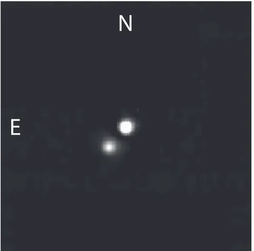
Figure 2.Speckle image of Kepler-14 with its obvious companion star separated by 0.3 of nearly equal brightness (∼0.5 mag fainter).
Table 1
Speckle Measurements of Kepler-14
Band Separationa Position Angleb Δ
mag
V 0.286±0.04 143.67±0.07 0.52±0.05
R 0.289±0.01 143.67±0.07 0.54±0.12
I 0.289±0.02 143.91±0.05 0.45±0.04
Notes.
aIn arcseconds. bIn degrees.
(2011). The latter presents details of the 2010 season of obser-vations for the KFOP.
A spatially close (0.3), nearly equal brightness (∼0.5 mag fainter) companion star was easily noted in the reconstructed speckle images. Table 1 gives the weighted mean values for the separation, position angle, and magnitude difference for our six speckle observations. The observations are weighted by the native seeing during the time of the speckle data collection as determined by the data reduction routines when fitting known single point-source speckle standard stars obtained near in time to the Kepler star observations. Figure 2 shows one of the reconstructed images of Kepler-14 with its obvious companion star.
3.2. High-resolution Palomar AO Imaging
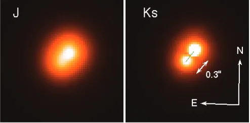
[image:2.612.317.570.358.409.2]Figure 3.JandKsPalomar adaptive optics images of Kepler-14, showing a 2×2field of view centered on the brighter star.
(A color version of this figure is available in the online journal.)
atKs. A total of 20 frames were acquired at J andKs for a total on-source integration time of 8.5 minutes and 4 minutes, respectively. The individual frames were reduced with a set of custom IDL routines written for the PHARO camera and were combined into a single final image. The adaptive optics system guided on the primary target itself; the widths of the central cores of the resulting point-spread functions (PSFs) were FWHM=0.15 atJand FWHM=0.1 atKs. The final co-added images atJandKsare shown in Figure3.
Other than the nearby object, two other sources were detected within 10of the primary target. The second closest object is separated from Kepler-14 by 5.5 to the northwest and has in-frared magnitudes ofJ =18.08±0.04 andKs =17.28±0.01. An additional source was detected to the southwest at a distance of 6.2 having infrared magnitudes ofJ = 19.00±0.05 and Ks =18.14±0.04.
The close pair was easily resolved by the adaptive optics at bothJandKs. The pair is separated by∼0.28 with a position angle of 142◦east of north. The pair has magnitude differences of ΔJ = 0.34±0.01 and ΔKs = 0.40±0.01. The brighter infrared (and optical) source (component A) is the northwestern star.
3.3. High-resolution ARIES AO Imaging
High-resolution AO images of Kepler-14 were obtained using the ARIES instrument on the 6.5 m MMT. ARIES is a near-infrared diffraction-limited imager and spectrograph. On 2009 November 8 it was operated in thef/15 mode, with a 40×40 field of view and a pixel scale of 0.04 pixel−1. All images of Kepler-14 had exposure times of 10 s, with 16 images inJ(in a four-point, 4dither pattern) and 19 images taken inKs(16 in a four-point, 4dither pattern, and 3 images at other offsets). The images for each filter were calibrated using standard IRAF28 procedures, and combined and sky-subtracted using the IRAF
taskxdimsum. The final co-added images atJandKsare shown
in Figure4.
In bothJandKs, the binary appearance of Kepler-14 is clear, with the fainter star, B, offset by 0.29±0.01 to the southeast. The separation is comparable to the image FWHM (0.5 in J and 0.3 inKs). The relative magnitudes were estimated by PSF fitting, yieldingΔJ =0.398±0.008 andΔK=0.490±0.005.
28 IRAF is distributed by the National Optical Astronomy Observatory, which is operated by the Association of Universities for Research in Astronomy, Inc., under cooperative agreement with the National Science Foundation.
Figure 4.MMT/ARIES AO images of Kepler-14 showing a 2.4×2.4 field of view inJandKsband. The binary nature of Kepler-14 is clear from the figure,
with the fainter star, B, offset by 0.29±0.01 to the southeast. (A color version of this figure is available in the online journal.)
The delta magnitudes from the Palomar and ARIES AO imaging are thus similar, but the difference of 0.06 mag in J and 0.09 mag inKs suggests that the accuracy is worse than implied by the formal precision. We combined all the Speckle and AO imaging results for the assessment of the dilution from the nearby companion.
3.4. High-resolution High S/N Spectroscopy
Spectroscopic observations of Kepler-14 were obtained using the FIbre-fed ´Echelle Spectrograph (FIES) at the 2.5 m NOT at La Palma, Spain (Djupvik & Andersen2010) as well as High Resolution Echelle Spectrometer (HIRES; Vogt et al. 1994) mounted on the Keck I telescope on Mauna Kea, Hawaii. We acquired 17 FIES spectra between 2009 August 4 and October 20, 3 of which were not used in the analysis because of very low S/N due to poor observing conditions. One HIRES template spectrum was also observed on 2009 September 10 and used to derive stellar parameters.
For HIRES, we set the spectrometer slit to 0.86, resulting in a resolving power ofλ/Δλ≈55,000 with a wavelength coverage of∼3800–8000 Å. We reduced the HIRES spectrum following a procedure based on that described by Butler et al. (1996).
[image:3.612.320.567.259.381.2]Table 2
Relative Radial-velocity Measurements of Kepler-14
HJD Phase RV σRV BS σBS
(days) (cycles) (m s−1) (m s−1) (m s−1) (m s−1)
2455048.454298 11.394 −246.1 25.0 21.4 7.4
2455052.427895 11.979 31.5 17.0 4.2 6.5
2455107.428247 20.079 −219.1 14.2 −6.8 4.9
2455108.417046 20.225 −385.2 15.4 −4.0 5.4
2455109.356436 20.363 −285.7 20.3 15.0 10.8
2455109.415242 20.372 −269.0 20.7 −1.7 5.3
2455111.453147 20.672 349.5 14.2 −30.5 6.9
2455112.462361 20.821 393.2 18.0 −41.2 8.7
2455113.456678 20.967 89.2 19.6 −5.8 7.0
2455114.494316 21.120 −260.0 25.6 18.4 6.3
2455115.492291 21.267 −404.0 30.2 51.2 11.0
2455122.475354 22.295 −387.8 20.3 −0.3 11.2
2455123.417485 22.434 −152.6 19.4 9.4 7.3
2455125.407529 22.727 398.5 19.4 −29.4 7.3
20 to 65 pixel−1(S/N of 38–120 per resolution element) over the wavelength range used. The rather large range in S/N is due to the variation in instrumental throughput and the stellar flux as a function of wavelength, and the lower throughput of the high-resolution fiber.
The FIES spectra were rectified and cross-correlated using a custom-built pipeline designed to provide precise RVs for
´
Echelle spectrographs. The procedures are described in more detail in Buchhave et al. (2010). The science exposures were bracketed by two thorium–argon (ThAr) calibration images taken through the same fiber and extracted using the same pipeline as the science exposures. The ThAr images were then combined to form the basis for the fiducial wavelength calibration. Once the spectra had been extracted, a cross-correlation was performed order by order using the strongest exposure as the template. The orders were cross-correlated using a fast Fourier transform and the cross-correlation functions (CCFs) for all the orders were co-added and fitted with a Gaussian function to determine the RV. Uncertainties of the individual velocities were estimated byσ =rms(v)/√N, where v is the RVs of the individual orders andNis the number of orders.
The light from the 0.5 mag fainter stellar companion (B) dilutes the light of the brighter star (A). In Section5.1, we use the photometric centroid to determine that it is the brighter star (A) which is undergoing transit and thus is the planet hosting star. The very small angular separation of 0.29 makes it impossible to separate the two stars on the fiber for spectroscopic observations and it is thus necessary to account for the effect of the dilution on the measured RVs (see Sections5.2and5.7).
In the observed FIES and HIRES spectra, we did not see a composite spectrum in any of the observations. We would easily have been able to identify two cross-correlation peaks from a composite spectrum, if the two stars did not have nearly equal RVs. The combination of the small angular separation of the two stars and the similar RV makes the probability of the two stars being a chance alignment highly unlikely, and we therefore conclude that the two stellar components are gravitationally bound in a wide orbit yielding an undetectable RV offset between the two spectra.
The RV measurements of the combined light of the two components in Kepler-14 are reported in Table 2. The RVs are relative, since they are measured relative to the strongest of the observed spectra adopted as the template. We made a
-400 -200 0 200 400
Radial velocity (m s
-1)
-400 -200 0 200 400
Radial velocity (m s
-1)
-50 0 50
Residuals (m s -1)
0.0 0.2 0.4 0.6 0.8 1.0
Phase -50
0 50
Bisector
var. (m s
-1)
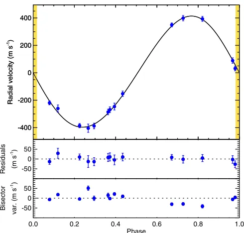
Figure 5.Upper panel: radial-velocity measurements from the FIbre-fed ´Echelle Spectrograph (FIES) at the 2.5 m Nordic Optical Telescope (NOT) at La Palma as a function of orbital phase with the best orbital fit overplotted. The velocity of the system has been subtracted and the fit assumes a circular orbit, fixing the ephemeris to that found by the photometry. Middle panel: phased residuals of the velocities after subtracting the best fit model. The rms variation of the residuals is 16.2 m s−1. Bottom panel: variations of the bisector span from the FIES spectra, with the mean value subtracted.
(A color version of this figure is available in the online journal.)
separate estimate of the systemic velocity (theγ velocity) by correlating the observed spectra against the synthetic library spectrum best matching the stellar parameters. We took the mean of these velocities and subtracted the gravitational redshift of the Sun (0.636 km s−1), which is not included in the calculation of the synthetic library spectra. We found the meanγ velocity of Kepler-14b to beγ =6.53±0.30 km s−1.
We fitted a circular orbit to the RVs reported in Table 2, adopting the photometric ephemeris, leaving only the orbital semi-amplitude,K, and an arbitrary RV offset as free parameters. A plot of the orbital solution is shown in the top panel in Figure5
with the residuals to the fit shown in the middle panel. The orbital parameters are listed in Table 3. Allowing the eccentricity to be a free parameter only reduced the velocity residuals by a small amount and yielded an eccentricity that was insignificant (e=0.035±0.020). However, we included the eccentricity in the light curve analysis in Section5.4mainly to allow for more realistic uncertainty estimates of the planetary parameters.
3.5. Bisector Analysis
We carried out a bisector span analysis (Queloz et al.2001; Torres et al.2007) of the FIES spectra to explore the possibility that the transit-like events are due to an eclipsing binary blended with light from a third star. The bisector spans are plotted in the bottom panel of Figure5.
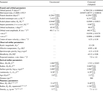
[image:4.612.43.295.75.249.2]Table 3
System Parameters for Kepler-14
Parameter Uncorrected Corrected
(Adopted)
Transit and orbital parameters
Orbital period,P(days)a,b . . . 6.7901230±0.0000043
Mid-transit time,E(HJD, UTC)a . . . 2454971.08737±0.00018
Transit duration (days)a,c 0.2561+0.0025
−0.0025 0.2591+0−0..00400039
Scaled semimajor axis,a/Ra,d 7.472+0−0.481.371 8.213
+0.578 −0.093
Scaled planet radius,Rp/Ra,d 0.0448−+00..00080002 0.0569±0.0013
Impact parameter,b≡acosi/Ra,d 0.531+0−0.088.078 0.00+0−0.41.00 Orbital inclination,i(deg)a,b 85.92+0.80
−0.92 90.0+0−2..08
Orbital semi-amplitude,K(m s−1)d,e 401.7±7.1 682.9+26.7
−24.6
esinωa,e . . . 0.0350±0.0170
ecosωa,e . . . 0.0006±0.0099
Center-of-mass velocity,γ(km s−1)e . . . 6.53±0.30
Observed stellar parameters
Keplermagnitude,Kpf . . . 12.128
Effective temperature,Teff(K)g . . . 6395±60
Spectroscopic gravity, logg(cgs)g . . . 4.11±0.10
Metallicity, [Fe/H]g . . . +0.12±0.06
Projected rotation,vsini(km s−1)g . . . 7.9±1.0
Derived stellar parameters
Mass,M(M )g,h 1.604−+00.057.060 1.512±0.043
Radius,R(R )g,h 2.358−+00.147.166 2.048+0−0.112.084
Surface gravity, logg(cgs)g,h 3.899−+00.049.041 3.994+0−0.028.036
Luminosity,L(L )g,h 8.30−+11.16.17 6.29+0−0.75.58
Age (Gyr)g,h 2.0+0.2
−0.2 2.2
+0.2 −0.1
Distance (pc)f,h . . . 980
Planetary parameters
Mass,Mp(MJ)a,d,e,g,h 5.14−+00.15.16 8.40+0−0.35.34 Radius,Rp(RJ, equatorial)a,d,e,g,h 1.036−+00.075.084 1.136+0−0.073.054
Density,ρp(g cm−3)a,d,e,g,h 5.7+1−1..50 7.1±1.1
Notes.
aBased onKeplerphotometry.
bThe actual orbital period differs fractionally from this value by (2.2±0.1)×10−5as a result of time dilation for the quoted gamma velocity.
cFirst to fourth contact point.
dBased on the dilution by the companion star. eBased on the FIES radial velocities. fBased on theKeplerInput Catalog.
gBased on an SME analysis on the HIRES spectra. hBased on the Girardi stellar evolution models.
would thus expect a positive bisector span when the host star is moving toward us and a negative bisector span when the host star is moving away. In the bottom planet in Figure5, we see a slight hint of this effect, with the bisector span being predominantly positive around phase 0.25 and predominantly negative around phase 0.75. The amplitude of the bisector spans is significantly less than the RV semi-amplitude and the hint of variation is in the expected direction, which supports the interpretation that the RV variations are due to a planetary companion.
4.WARM-SPITZEROBSERVATIONS
Kepler-14 was observed during one transit with
Warm-Spitzer/IRAC (Werner et al.2004; Fazio et al.2004) at 4.5μm
(program ID 60028). The observation occurred on UT 2010 August 7 and the visit lasted approximately 14 hr 20 minutes.
The data were gathered in full-frame mode (256×256 pixels) with an exposure time of 30 s per image, which yielded 1700 images.
Figure 6.Warm-Spitzertransit light curve of Kepler-14 observed in the IRAC bandpass at 4.5μm. Top panel: raw and unbinned transit light curve. The red solid lines correspond to the best-fit models which include the time and position instrumental decorrelations as well as the model for the planetary transit (see details in Section4). Middle panel: corrected, binned by 35 minutes, and normalized transit light curve with the best fit in red. Bottom panel: residuals of the data from the best fit.
(A color version of this figure is available in the online journal.)
TDB-based BJD using theUTC2BJD29procedure developed by Eastman et al. (2010). This program uses the JPL Horizons ephemeris to estimate the position of theSpitzer Space Telescope during the observations. We then correct for transient pixels in each individual image using a 20 point sliding median filter of the pixel intensity versus time. To do so, we compare each pixel’s intensity to the median of the 10 preceding and 10 following exposures at the same pixel position and we replace outliers greater than 4σ with its median value. The fraction of pixels we correct is less than 0.06%. The centroid position of the stellar PSF is determined using a DAOPHOT-type Photometry Procedure,GCNTRD, from the IDL Astronomy Library.30We use theAPERroutine to perform aperture photometry with a circular aperture of variable radius, using radii of 1.5–8 pixels, in 0.5 steps. The propagated uncertainties are derived as a function of the aperture radius; we adopt the one which provides the smallest errors. We find that the transit depths and errors vary only weakly with the aperture radius for all the light curves analyzed in this project. The optimal aperture is found to have a radius of 4.0 pixels. We estimate the background by fitting a Gaussian to the central region of the histogram of counts from the full array. The contribution of the background to the total flux from the stars is low for both observations, from 0.1% to 0.55% depending on the images. Therefore, photometric errors are not dominated by fluctuations in the background. We used a sliding median filter to select and trim outliers in flux and position greater than 5σ. We also discarded the first half-hour of observations, which are affected by a significant telescope jitter before stabilization. The final number of photometric measurements used is 1570. The raw time series is presented in the top panel of Figure6. We find that the point-to-point scatter in the photometry gives a typical S/N of 330 per image, which corresponds to 92% of the
29 http://astroutils.astronomy.ohio-state.edu/time/ 30 http://idlastro.gsfc.nasa.gov/homepage.html
theoretical signal-to-noise. Therefore, the noise is dominated by Poisson photon noise.
5. ANALYSIS 5.1. Centroid Shifts
We use a comparison of the photometric centroid in- and out-of-transit data from Kepler to determine which component contains the transit event. These centroids have been measured for quarters 1–6 using two methods: (1) a fit of the transit model to the whitened row and column centroid time series, which provides an average offset in row and column for each quarter, and (2) centroiding of quarterly average in- and out-of-transit images, where the transit average is constructed from all in-transit observations in a quarter and the out-of-in-transit average is constructed from placing the same number of points on each side of each transit event.
Both methods measured essentially identical centroid offsets. These offsets were used to reconstruct the position on the sky of the transiting object, using the methods described in Appendix A of Jenkins et al. (2010a). The final reconstructed transit source location is then the average of the reconstructed transit position over all quarters. The distance of this average reconstructed position from component A is 0.025±0.024 (1.04σ) and from component B is 0.251±0.030 (8.33σ). We conclude that the transiting object is component A.
5.2. Spectroscopic Parameters of the Host Star
As noted in Section3.4, we cannot separate the two stellar components on the fiber of the spectrograph and we thus observed the light from both stars in the spectra. As argued in Section 3.4, we assumed that the two stars are physically associated and that they formed together at the same time. Since the stars have nearly the same temperature due to their position on the HR diagram, we concluded that the small magnitude difference would result in an insignificant change in the host star parameters (see Section5.3for details).
We derived stellar atmospheric parameters from both the HIRES template spectrum and the high S/N FIES spectra used for the orbit determination, which can all be used because they are not contaminated by absorption from an iodine cell.
For the HIRES spectrum, we used an analysis package known as Spectroscopy Made Easy (SME; Valenti & Piskunov
1996), along with the atomic line database of Valenti & Fischer (2005). From the HIRES spectrum using SME, we found the following parameters: effective temperatureTeff = 6395±60 K, metallicity [Fe/H]=+0.12±0.06 dex, projected rotational velocityvsini=7.9±1.0 km s−1, and stellar surface gravity logg=4.11±0.10 (cgs).
5.3. Properties of the Host Star
Global properties of the star including the mass and radius were determined with the help of the stellar evolution models from the series by Girardi et al. (2000). Isochrones for a wide range of ages were compared against the effective temperature and metallicity from the Keck/HIRES spectra, and the mean stellar density,ρ, as an indicator of luminosity. If we assume a circular orbit, then the mean stellar density is closely related to the normalized semimajor axis a/R (see, e.g., Seager & Mall´en-Ornelas2003; Sozzetti et al.2007), which is one of the parameters solved for in the light curve solutions described below in Section 5.4, and is often more accurate than the spectroscopic logg. In practice we used a/R rather thanρ, and the comparison with the isochrones was coupled with the light curve solutions, which were carried out using the Markov Chain Monte Carlo technique. Specifically, we derived
adistributionof stellar properties by comparing the isochrones
with each value in thea/Rchains paired with values for the temperature and metallicity drawn from Gaussian distributions centered on the spectroscopically determined values and their errors.
The presence of the visual companion detected in our high-resolution imaging adds a complication, as the extra flux reduces the depth of the transit and affects its overall shape in subtle ways, biasing the a/R parameter. The impact of this extra dilution depends on the magnitude difference of the companion in the Kepler band (ΔKp), which we expect to be close to (but not necessarily the same as) the measured magnitude differences in other passbands (ΔV, ΔR, ΔI, ΔJ, andΔKs). We therefore proceeded by iteration, in parallel with the light-curve solutions. We initially ignored the dilution effect ona/R, and inferred the absolute magnitude of the target in the Kp band from the best-fit isochrone. Assuming the companion is physically associated and the two stars share the same isochrone, we then determined its mass along the isochrone with the condition that the magnitude difference inVbe exactly equal to the measured value. We then read off theΔKpvalue directly from the isochrone. We repeated this using each of the other magnitude difference measurements (taking those inJandKs from the MMT and Palomar to be independent), and we averaged the resulting seven values ofΔKpto obtain 0.45±0.10 mag. With the corresponding relative fluxFB/FAa new light curve solution was carried out, leading to an improved a/Rdistribution. This, in turn, was compared once again with the isochrones and led to a slightly revised brightness difference ofΔKp=0.44±0.10 mag. A further iteration did not change this significantly.
As described in Section5.2, we have determined the host star parameters from the composite spectra of the primary star A and the fainter companion B, since it is not possible to separate the two stars on the fiber/slit of the spectrographs. We estimate that the adopted magnitude difference ofΔKp=0.44±0.10 mag does not significantly affect the derived spectroscopic stellar properties of the host star A. The companion star B is estimated to be only 30 K hotter and have a stronger surface gravity of 0.15 dex compared to the host star. We therefore choose to ignore the effect of the dilution on the stellar parameters of the host star.
The resulting properties of the host star are listed in Table3, in which the values correspond to the mode of the distributions and the uncertainties reported are the 68.3% (1σ) confidence limits defined by the 15.8% and 84.2% percentiles in the cumulative distributions.
We estimated the distance to Kepler-14 based on isochrones by comparing against the measured magnitudes from theKepler Input Catalog (Brown et al.2011). We fitted the spectral energy distribution with magnitudes for the two stars taken from the Girardi isochrones resulting in a distance estimate of 980 pc. For an average angular separation of 0.29 the semi-major axis of the visual pair is approximately 280 AU, and with mass estimates of 1.51M and 1.39M for the two stars, the corresponding period is on the order of 2800 years.
5.4. Light-curve Analysis
We modeled the folded transit light curve assuming spherical star and planet having radius ratioRp/R. The second star adds its light to the total light curve with the observed flux ratio between stars B and A beingFB/FA. The planet was constrained to a circular Keplerian orbit parameterized by a period P, a normalized semi-major axis distancea/R,and an inclination to the sky planei.
The normalized transit light curve,f(t), was calculated to be
f(t)=1−λ
z(t)/R, Rp R
, u1, u2
1 +FB FA
, (1)
wherez(t) is the sky-projected separation of the centers of the star and planet andλis the fraction of the stellar disk blocked by the planet, given analytically by Mandel & Agol (2002). The limb-darkening coefficients u1 andu2 parameterize the radial brightness profile,I(r), of a star as
I(r)
I(0) =1−u1
1−1−r2 −u 2
1−1−r2 2. (2)
The continuously defined model, f(t), was numerically integrated before being compared with the long cadenceKepler light curve. In detail, for each measured time, tj, we take nj uniform samples tj,k = tj + kΔtj −τint/2, separated by
Δtj = τint/nj, over the long cadence integration interval of τint=29.4 minutes. The flux attjwas found by computing the Gaussian quadrature of the continuous model fluxesf(tj,k). In practice, we tooknj =20 for all times.
We determined the best-fit model to the data by minimizing theχ2goodness-of-fit statistic including Gaussian penalties to restrict the flux ratioFB/FA,ecosω, andesinωto agree with the observed constraints:
χ2=
s
(Fs−Fs)2
σ2 +
(FB/FA−0.667)2 0.0612
+ (esinω−0.035) 2
0.0172 +
(ecosω−0.0006)2
0.00992 , (3)
the number of links was much larger than the autocorrelation length (equal to the number of links at which the chain auto-correlation drops below one half) for any selected parameter. We report the 15.8% and 84.2% values of the cumulative dis-tribution for each parameter, marginalizing over the remaining parameters.
5.5. Analysis of the Warm-Spitzer Light Curves
We used a transit light-curve model multiplied by instrumen-tal decorrelation functions to measure the transit parameters and their uncertainties from theWarm-Spitzerdata as described in D´esert et al. (2011b). We computed the transit light curves with the IDL transit routineOCCULTNLfrom Mandel & Agol (2002). This function depends on one parameter: the planet-to-star radius ratioRp/R. The orbital semi-major axis to stellar radius ratio (system scale)a/R, the impact parameterb, and the time of mid-transitTcwere fixed to the values derived from the
Keplerlight curve and corrected for the dilution (see Table3).
We assumed that the limb darkening is well approximated by a nonlinear law at infrared wavelengths with four coefficients (Claret 2000) that we set to their values computed by Sing (2010).
The Spitzer/IRAC photometry is known to be
systemati-cally affected by the so-called pixel-phase effect (see, e.g., Charbonneau et al.2005; Knutson et al. 2008). This effect is seen as oscillations in the measured fluxes with a period of ap-proximately 70 minutes (period of the telescope pointing jitter) and an amplitude of approximately 2% peak-to-peak. We decor-related our signal in each channel using a linear function of time for the baseline (two parameters) and a quadratic function of the PSF position (four parameters) to correct the data for each channel. We performed a simultaneous Levenberg–Marquardt least-squares fit (Markwardt2009) to the data to determine the transit and instrumental model parameters (seven in total). The errors on each photometric point were assumed to be identical and were set to the rms of the residuals of the initial best fit obtained. To obtain an estimate of the correlated and system-atic errors (Pont et al.2006) in our measurements, we used the residual permutation bootstrap, or “Prayer Bead,” method as de-scribed in D´esert et al. (2009). In this method, the residuals of the initial fit are shifted systematically and sequentially by one frame, and then added to the transit light-curve model before fitting again. We allowed asymmetric error bars spanning 34% of the points above and below the median of the distributions to derive the 1σ uncertainties for each parameter as described in D´esert et al. (2011a).
5.6. Interpretation of the Warm-Spitzer Observations
We compute the theoretical dilution factor by extrapolating theKs-band measurements to theSpitzerbandpass at 4.5μm. We estimate that 36% of the photons recorded during the observation come from the companion star. We conclude that the presence of the contaminating star decreases the effective transit depth of Kepler-14 by a factor 0.61. We measure the transit depth (limb-darkening removed) of Kepler-14 at 4.5μm and find 1722+127−138ppm uncorrected for the dilution. This corresponds to Rp/R = 0.0415+0.0015−0.0017. Applying the dilution correction, we findRp/R=0.0531+0.0019−0.0021, which is consistent with the value derived from theKeplerphotometry at better than the 2σ level.
OurSpitzerobservations provide an independent confirmation
that the transit signal is achromatic, which supports the planetary nature of Kepler-14b.
0.0 0.2 0.4 0.6 0.8 1.0
FB/FA
300 400 500 600 700 800
Vcor
(m s
[image:8.612.335.550.55.192.2]-1)
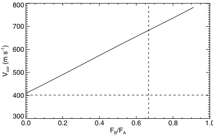
Figure 7.Effect of the dilution of Kepler-14 on the measured radial velocities as a function of flux ratio between the companion star and the host star. The horizontal dashed line represents the observed semi-amplitude of the system and the vertical dashed line represents the adopted flux ratio of the two stars. If the stars have the same brightness, the corrected radial velocity is about twice the observed, and at large magnitude differences, the corrected velocities approach the observed, as expected.
5.7. Dilution Effect on the Radial Velocities
The measured RVs of the host star (A) are affected by the light contributed by the companion star (B), because the spectrum of B is assumed to be stationary in velocity, while the spectrum of A is Doppler-shifted due to the gravitational pull of the planet. The amplitude of the observed RVs will thus be smaller than if the light from A had not been diluted, since the peak of the CCF from which we derive the RVs will be pulled toward the stationary CCF of B.
In order to assess the dilution effect on the RVs and thus the semi-amplitude of the orbit, we modeled the effect using the observed spectrum of Kepler-14. We shifted the observed spectrum in 50 m s−1 increments and co-added the shifted spectrum, representing star A, with the same observed spectrum divided by a constant to simulate the stationary companion B at different flux ratios off =FB/FA. We analyzed this composite spectrum using the same tools used to extract the RVs for the orbit.
The relation between the artificially induced RV shifts, Vin, and the resulting “measured” RV shifts of the composite spectrum,Vout, is linear at given flux ratio, as expected:Vout = afVin, where af is the slope at a given flux ratio. Vin thus represents the true (corrected) RVs of the host star (Vcor) and Voutrepresents the observed RVs of the host star (Vobs).
We carried out this analysis at different flux ratios, fitting the linear relation betweenVinandVout, and thus obtaining the slope af at each flux ratio. We then fitted the slopes,af, themselves as a function of flux ratio with a third-order polynomial. This enables us to calculate the dilution effect for the system at any flux ratio:
Vcor= Vobs
af
= Vobs
c0+c1f +c2f2+c 3f3
, (4)
and at large magnitude differences, the corrected RV approaches the observed RVs, as expected.
The observed orbital semi-amplitude of Kepler-14 isKobs= 401.7 ±7.1 m s−1. Since the two stars are nearly the same temperature, the dilution changes only minutely as a function of wavelength. We thus used the magnitude difference ofΔKp= 0.44±0.10 in all orders and found the corrected semi-amplitude of the orbit to beKcor =682.9+26.7−24.6m s−1. We propagated the uncertainty of the adopted magnitude difference and added it in quadrature with the uncertainty of the uncorrected semi-amplitude. The correction assumes that the two stars have the same rotational broadening of the lines in their spectra and that the velocity shift between the two stars (due to motion in their wide orbit around each other) is small enough to be ignored. In the unlikely case that the companion star is rotating very rapidly, our model would overcorrect the velocity amplitude due to dilution. However, there is no evidence in the CCF for a broad secondary peak.
5.8. Dilution Effect on the Planetary Parameters
The dilution of the nearly equal magnitude stellar companion significantly affects the derived planetary parameters of Kepler-14b. The contamination affects the observed transit light-curve depth and therefore the inferred radius ratio. In addition, this dilution has a significant effect on the light-curve profile affecting the inferred geometric orbital parameters, most notably the normalized semi-major axis,a/R. If dilution effects are neglected, the mean stellar density estimate—which is acutely sensitive to a/R—used in conjunction with spectroscopic stellar constraints will yield significantly inaccurate derived stellar properties.
If we assume that the flux contribution from B is zero (i.e., FB/FA = 0 and Kobs = 401.7±7.1 m s−1), we find that Rp,nocorr = 1.036+0.075−0.084RJ. Using the derived magnitude differenceΔKp=0.44±0.10, however, we find the planetary radius to beRp=1.136+0.073−0.054RJ, which is almost 10% larger.
As described in Section5.7, the orbital semi-amplitude is also significantly affected by the dilution. Using the observed orbital semi-amplitude of Kobs=401.7 ±7.1 m s−1, the un-corrected mass of Kepler-14b is Mp,nocorr = 5.14+0.15−0.16MJ. After correction for dilution, the semi-amplitude increases to Kcorr=682.9+26.7
−24.6m s−1, which in turn leads to a plane-tary mass that is significantly larger than before (by∼60%): Mp =8.40+0.35−0.34MJ.
The effect of the dilution is much greater on the mass than on the radius of the transiting planet. As described above, the dilution of the observed transit light curve changes not only the depth of the transit, but also the light-curve profile which in turn affects the inferred stellar density estimate. The radius of the planet is thus not affected greatly by the dilution, because these two effects work against each other. The stellar mass, however, is not strongly affected by the dilution and the effect on the planetary mass therefore comes almost entirely from correction of the orbital semi-amplitude.
6. DISCUSSION
We present the discovery of a transiting hot-Jupiter in a close visual binary. Had the visual companion not been detected, the planetary parameters for Kepler-14b would have been significantly biased. The dilution (ΔKp = 0.44±0.10 in the
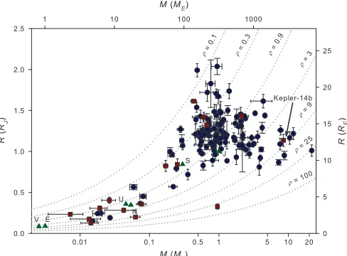
[image:9.612.322.566.56.236.2]Keplerband) results in a planetary mass that, if left uncorrected,
Figure 8.Mass–radius diagram of currently known transiting exoplanets.Kepler planets are shown as red squares and planets from other surveys are shown as blue circles. The solar system planets are shown as green triangles. The dotted lines are isodensity curves (in g cm−3). Kepler-14 is one of the most massive transiting exoplanets discovered.
is only 60% of the correct value, and a planetary radius that is too small by about 10%.
The close angular separation of this physically associated vi-sual companion makes it essentially undetectable spectroscop-ically: the RV similar to the main star means the spectrum is effectively single-lined, and the wide orbit (P ∼2800 yr) im-plies motion that is slow enough that there are no measurable changes in the velocity of the primary due to this companion. It is only with high-resolution imaging that we were able to detect it. Many of the over 120 published transiting planets and the over 500 published RV planets have not been subjected to high-resolution imaging. It is thus possible that some of the published exoplanets have incorrectly determined planetary parameters, if they have a stellar companion like Kepler-14 and the companion has not been taken into account. Since many of the published transiting planets have bright host stars, a campaign to gather high-resolution imaging of the host stars could be carried out with a modest amount of telescope time.
In this paper, we confirm and characterize the planetary nature of Kepler-14b, also known as KOI-98 in Borucki et al. (2011). Kepler-14b has a period of P = 6.7901230± 0.0000043 days, a mass of Mp = 8.40+0.35−0.34MJ, and a ra-dius of Rp = 1.136+0.073−0.054RJ, yielding a mean density of ρp = 7.1 ± 1.1 g cm−3. Not taking the dilution into ac-count, the derived mass and radius of the planet would be Mp,nocorr=5.14+0.15−0.16MJandRp,nocorr =1.036+0.075−0.084RJ.
Kepler-14b is plotted on a mass–radius diagram in Figure8, which shows all the known transiting exoplanets. Kepler-14b is one of the most massive transiting exoplanets discovered and is situated in a less dense part of the mass–radius diagram together with six other planets of similar mass.
which is operated by the Jet Propulsion Laboratory, California Institute of Technology under a contract with NASA. Support for this work was also provided by NASA through an award issued by JPL/Caltech.
Facilities: Kepler, NOT (FIES), Keck:I (HIRES), Spitzer,
WIYN (Speckle), Hale, MMT
REFERENCES
Borucki, W. J., Koch, D., Basri, G., et al. 2010,Science,327, 977
Borucki, W. J., et al. 2011,ApJ,736, 19
Brown, T. M., Latham, D. W., Everett, M. E., & Esquerdo, G. A. 2011, arXiv:1102.0342
Buchhave, L. A., Bakos, G., Hartman, J. D., et al. 2010,ApJ,720, 1118
Butler, R. P., Marcy, G. W., Williams, E., et al. 1996,PASP,108, 500
Charbonneau, D., Allen, L. E., Megeath, S. T., et al. 2005,ApJ,626, 523
Claret, A. 2000, A&A,363, 1081
D´esert, J.-M., Lecavelier des Etangs, A., H´ebrard, G., et al. 2009,ApJ,699, 478
D´esert, J.-M., Sing, D., Vidal-Madjar, A., et al. 2011a,A&A,526, A12
D´esert, J.-M., et al. 2011b, arXiv:1102.0555
Djupvik, A. A., & Andersen, J. 2010, in Highlights of Spanish Astrophysics V, ed. J. M. Diego et al. (Berlin: Springer),211
Eastman, J., Siverd, R., & Gaudi, B. S. 2010,PASP,122, 935
Fazio, G. G., Ashby, M. L. N., Barmby, P., et al. 2004,ApJS,154, 39
Girardi, L., Bressan, A., Bertelli, G., & Chiosi, C. 2000,A&AS,141, 371
Hayward, T. L., Brandl, B., Pirger, B., et al. 2001,PASP,113, 105
Horch, E. P., Gomez, S. C., Sherry, W. H., et al. 2011,AJ,141, 45
Howell, S. B., Everett, M. E., Sherry, W., Horch, E., & Ciardi, D. R. 2011,AJ,
142, 19
Jenkins, J. M., Borucki, W. J., Koch, D. G., et al. 2010a,ApJ,724, 1108
Jenkins, J. M., Caldwell, D. A., Chandrasekaran, H., et al. 2010b,ApJ,713, L120
Jenkins, J. M., Caldwell, D. A., Chandrasekaran, H., et al. 2010c,ApJ,713, L87
Knutson, H. A., Charbonneau, D., Allen, L. E., Burrows, A., & Megeath, S. T. 2008,ApJ,673, 526
Koch, D. G., Borucki, W. J., Rowe, J. F., et al. 2010,ApJ,713, L131
Mandel, K., & Agol, E. 2002,ApJ,580, L171
Markwardt, C. B. 2009, in ASP Conf. Ser. 411, Astronomical Data Analysis Software and Systems XVIII, ed. D. A. Bohlender, D. Durand, & P. Dowler (San Francisco, CA: ASP),251
Pont, F., Zucker, S., & Queloz, D. 2006,MNRAS,373, 231
Queloz, D., Henry, G. W., Sivan, J. P., et al. 2001,A&A,379, 279
Seager, S., & Mall´en-Ornelas, G. 2003,ApJ,585, 1038
Sing, D. K. 2010,A&A,510, A21
Sozzetti, A., Torres, G., Charbonneau, D., et al. 2007,ApJ,664, 1190
Ter Braak, C. 2006,Stat. Comput., 16, 239
Torres, G., Neuh¨auser, R., & Guenther, E. W. 2002,AJ,123, 1701
Torres, G., Bakos, G. ´A., Kov´acs, G., et al. 2007,ApJ,666, L121
Troy, M., Dekany, R. G., Brack, G., et al. 2000,Proc. SPIE,4007, 31
Valenti, J. A., & Fischer, D. A. 2005,ApJS,159, 141
Valenti, J. A., & Piskunov, N. 1996,A&AS,118, 595
Vogt, S. S., Allen, S. L., Bigelow, B. C., et al. 1994,Proc. SPIE,2198, 362

![Crystal structure of 2 {[2 (3 phenylallylidene)hydrazin 1 yl]thiocarbonylsulfanylmethyl}pyridinium chloride](data:image/gif;base64,R0lGODlhAQABAIAAAP///wAAACH5BAEAAAAALAAAAAABAAEAAAICRAEAOw==)