PRICING ENDOWMENTS WITH SOFT COMPUTING

(1)

Jorge DE ANDRÉS-SÁNCHEZ, PhD

E-mail: [email protected]

Society and Business Research Laboratory

Rovira i Virgili University

Laura GONZÁLEZ-VILA PUCHADES, PhD

E-mail: [email protected]

Department of Economic, Financial and Actuarial Mathematics University of Barcelona

PRICING ENDOWMENTS WITH SOFT COMPUTING

Abstract: This paper develops life insurance pricing with different representation of its two sources of uncertainty: stochastic behaviour of mortality of the insured and fuzzy quantification of interest rates within the time horizon. Concretely we analyse endowment contracts, which are present in several financial real-world contexts as residential mortgage loans or retirement plans. We show that modelling the present value of these contracts with fuzzy random variables allows a well-founded quantification of their fair price and the risk resulting from the uncertainty of mortality and discounting rates. To do this, we firstly describe fuzzy random variables and some associated measures (mathematical expectation, variance, distribution function and quantiles) are defined. Subsequently the present value of a endowment contract (pure and mixed) is modelled with fuzzy random variables. Finally we show how the price and risk measures for endowment portfolios can be obtained.

Keywords:Life insurance, endowment, stochastic mortality, fuzzy interest rate, fuzzy random variable.

(2)

Jorge De Andrés-Sánchez, Laura González-Vila Puchades

__________________________________________________________ 1. Introduction

Life insurance pricing has to model the uncertainty of demographic events and financial parameters. From its beginning, actuarial science has paid much attention to quantifying demographic phenomena and its stochastic uncertainty. In fact, its probabilistic behaviour is commonly accepted and practitioners obtain the corresponding probabilities from life tables. However, from 70s several authors introduce the uncertainty related to the financial parameters (specially the discount rate used to price contracts) by means of random variables (RV) and stochastic processes (see for example [Boyle, P.P., 1976]). From these papers a lot of contributions appeared, using different approaches but agreeing on the consideration of the stochastic nature of the interest rate.

From 90s some contributions like [Lemaire, J., 1990] and [Ostaszewski, K., 1993] also propose the use of some appropriate instruments of the Fuzzy Set Theory (FST) to model the behaviour of interest rate. In this respect, the papers published later [Andrés-Sánchez, J., Terceño, A., 2003] and [Betzuen, A., Jiménez, M., Rivas, J.A., 1997] are particularly noteworthy.

Most of papers on fuzzy actuarial pricing reduce the randomness of the behaviour of claiming processes to predefined frequencies – i.e. the randomness of the present value of premiums and benefits is reduced to its mathematical expectation – and, therefore, these processes become deterministic. On one hand, this approach allows insurance contracts to be priced by automatically applying the financial mathematics with fuzzy parameters developed in [Buckley, J.J., 1987], [Kaufmann, A., 1986] and [Li Calzi, L., 1990]. On the other, the information that provides the complete statistical description of claiming is lost, making it hard to rigorously introduce the uncertainty of claiming when fitting magnitudes like reserves for deviations of mortality or premium surplus. In this paper we develop an approach to price endowment contracts that combines the stochastic approach to life insurance mathematics (see [Gerber, H.U., 1995] under deterministic interest rates) and the quantification of interest rates with fuzzy numbers (FNs), following the developments in [Andrés-Sánchez, J., González-Vila, L., 2012]. Our approach will therefore allow us to maintain stochastic and fuzzy sources of uncertainty throughout all of the valuation processes. Related to our fuzzy methodology, [Shapiro, A., 2009] describes fuzzy random variables with actuarial modelling in view and [Huang, T., Zhao, R., Tang, W., 2009] develops a non-life individual risk model where the number of claims follows a Poisson process whereas their value is estimated with a triangular fuzzy number (TFN).

We have structured this paper as follows. In sections 2 we describe the concepts and instruments of FST on which our approach is based. In section 3 we calculate price of endowment policies with a fuzzy random approach whereas in section 4 we evaluate endowment portfolios.

(3)

Pricing Endowments with Soft Computing

__________________________________________________________ 2. Fuzzy random variables

In many real situations the uncertainty is the result any one of numerous different causes: randomness, hazard, inaccuracy, incomplete information, etc. The concept of Fuzzy Random Variable (FRV) combines both random and fuzzy uncertainty: [Krätschmer, V., 2001], [Kruse, R., Meyer, K.D., 1987], [Kwakernaak, H., 1978 and 1979], [Puri, M.L., Ralescu, D.A., 1986] and [Zhong, C., Zhou, G., 1987], but there is not a unique definition for it. This paper uses [Puri, M.L., Ralescu, D.A., 1986] because it is very suitable for modelling the present value of life insurance contracts. When pricing life insurances the randomness is due to the demographical phenomenon in such a way that the moment in which the benefit is paid can be described with a conventional RV. Likewise, the outcomes of the present value of life insurance will not be real but fuzzy numbers because we suppose that discount rates used to calculate present values are estimated by means of generalized intervals.

Let

,

A

be a measurable space,

, B

the Borel measurable space and F( ) denote the set of FNs. The fuzzy set valued mapping

X

:

: F( )

is called a fuzzy random variable if:

B B, 0,1 , |X B A

where

X

is a FN that must be viewed as a generalized interval with membership function _X z and -level representation:

| ,

X z _X z X X

[Guangyuan, W., Yue, Z., 1992] demonstrates that any FRV

X

defines,

0,1

, an infima RV X and a suprema RV X whose realizations are, respectively, the lower and upper extremes of -cuts of

,

X

,

X

,

X

.

Let

,

A

,

P

be a probability space. Given that in our paper we will price discrete life insurances, the next definitions are referred to discrete FRVs that

(4)

__________________________________________________________

come from the set of elemental outcomes _{i i} _{1, ,}_n with

,

1,

,

i i

P

p

i

n

.

Let

X

be a discrete FRV on

,

A

,

P

, being F_X and F_X ,

0,1

, the distribution functions of the RVs X and X obtained from

X

. Then, , we define the couple of the distribution functions of the RVs infima and suprema for that membership level F_X x = F_X x ,F_X x :

F

_X

x

P

X

x

F

_X

x

, F_X x P X x F_X x (1)

Likewise, for a discrete FRV

X

with F_X and F_X ,

0,1

, being the distribution functions of the probability of the RVs X and X obtained from

X

, we define the couple of th quantiles of the RVs infima and suprema for that membership level

Q

,

Q

X X X :

min

|

Q

x F

_X

x

X and

Q

X

min

x F

|

X

x

(2)

In the case that _i ,i 1, ,n, the FNs

X

_i satisfy,

0,1

, X _i X _i ₁ and X _i X _i ₁ , i 1, ,n 1, for

Q

X we find:

min

_i

|

_j i _{j i}

Q

X

p

X and

min

_i i

|

j j i

Q

X

p

X

Given the probability space

,

A

,

P

with _{i i} _{1, ,}_n and

,

1,

,

i i

P

p

i

n

, the mathematical expectation of a discrete ordinary RV X is a function of its realizations {x1, x2,...,xn}: ₁ ₂

1 , ,..., n n i i i E X x x x x p .

So, given a FRV

X

its mathematical expectation, , is the FN induced by the FNs X( ₁),X( ₂), ,X( _n) through

E

X

. Concretely, following [Puri,

(5)

__________________________________________________________

M.L., Ralescu, D.A., 1986] we can compute the extremes of the -cuts of ,

,

E

X

E

X

E

X

,

0,1

as: 1 1 , , n n i i i i i i E X X p X p E X E X (3)

Regarding the variance of FRVs some authors propose fuzzy definitions, as in the case of mathematical expectation, whereas other authors such as [Feng, Y., Hu, L., Shu, H., 2001] and [Körner, R., 1997] propose using scalar (crisp) values for the variance since it is a dispersion measure. This dichotomy in the definition makes that a choice of one definition must be done (for a more detailed discussion of this topic see [Couso, I., Dubois, D., Montes, S., Sánchez, L., 2007]. Due to the choice we have made of the FRV concept we will expose the concept of variance contained in [Feng, Y., Hu, L., Shu, H., 2001] that is built up from the variance of the infima and suprema RVs X and X obtained from

X

So, for a discrete FRV

X

with infima and suprema discrete RVs X and X ,

0,1

, the variance of

X

,V X , is the real number:

1

0

1 2

V X V X V X d (4)

Of course, from this definition of the variance of a FRV we can derive a crisp standard deviation as

D

X

V

X

.

Notice that we use the superscript “ ” to symbolise fuzzy magnitudes and we write random variables with bold letters. So, the symbols corresponding to fuzzy random variables will be in bold and contain the superscript “ ”.

3. Pricing endowment policies with fuzzy random variables

Following [Andrés-Sánchez, J., González-Vila, L., 2012] we propose adapting the stochastic approach to life insurance contracts to the use of fuzzy discount rates. In this case, the RV present value of premiums and present value of benefits turn into FRVs that will allow us to maintain all the uncertainty associated with discount rates but also with mortality. Considering that the discount rates are given via FNs, the value of discount function for 1 monetary unit (m.u.) payable at

(6)

__________________________________________________________

t is a FN,

d

_t, with α-cut representation

d

_t

d

_t

,

d

_t . Notice that [Andrés-Sánchez, J., González-Vila, L., 2012] exposes several ways to estimate actuarial discount rates with FNs.

Let us consider the simple case of an n-year pure endowment for a person aged x years. In this case the insured will receive 1 m.u. if he survives n years and no amount otherwise. The space of events is ={ 0, 1} where 0= “the insured

survives n years (and so perceives 1 m.u.)” and 1= “the insured dies within the

next n years (and so does not perceive the insured amount)”.

From the discount function

d

_t,we can generate the FRV present value of pure endowment associated to a person aged x years

x:n

A ₁ . The outcomes of this FRV are random because they depend on the insurer’s death age. But these outcomes are also FNs since they are calculated with fuzzy discount rates that are generalized intervals. This FRV adopts as values the following FNs, with respective probabilities P: outcomes 0 1 _n _x n n x P p d p

being _np_x the probability that the insured aged x will survive n years. The FRV

x:n

A ₁ defines, , the infima and suprema RVs

x:n A ₁ and x:n

A

₁ as: outcomes 0 1 _n _x n n x P p d p x:n A ₁ outcomes 0 1 _n _x n n x P p d p x:n A ₁

Based on the concepts defined in section 2, contained in (1) to (4), we can determine the next magnitudes.

(7)

__________________________________________________________ -cuts of the mathematical expectation of the FRV

x:n A ₁ .

0,1

,

E

x:n

A

₁ =

E

,

E

x:n x:n

A

₁

A

₁ , with: n n x E ₁ E ₁ d p x:n x:n A A n n x

E

₁

E

₁

d

p

x:n x:n

A

Variance and standard deviation of the of the FRV

x:n

A ₁ .

The variances of the RVs

x:n A 1 and 1 x:n

A

are: 2 2 2 1 n n x n n x n n x n x V 1 d p d p d p p x:n A 2 2 2 1 n n x n n x n n x n x V d p d p d p p x:n A 1

So the variance of the FRV

x:n A ₁ is: 1 ₂ ₂ 0

1

2

n n n x n x

V

₁

d

p

d

x:n

A

being its standard deviation D V x:n x:n

(8)

__________________________________________________________ Couple of distribution functions of the RVs

x:n A ₁ and 1 x:n

A

,

0,1

. Considering (1),

0,1

, _F _y _F _y _,_F _y x:n x:n x:n A ₁ A ₁ A ₁ Notice that F y 1 x:n A F ₁ y x:n

A can be obtained from the

distribution function of the RV 1

x:n

A

₁ x:n A . So:

0

if

0

1

if

0

1

if

n x n n

y

F

y

p

y

d

y

d

x:n A ₁ (5a) 0 if 0 1 if 0 1 if n x n n y F y p y d y d x:n A ₁ (5b)

Couple of th quantiles of the RVs

x:n

A ₁ and ₁

x:n

A

,

0,1

.

From (5a) and (5b) the couples are

Q

,

Q

x:n x:n x:n A ₁ A ₁ A ₁ : - If 0 1 _n p_x: Q 0, 0 x:n A ₁ - If 1 _n p_x 1: Q d_n ,d_n x:n A ₁

(9)

__________________________________________________________

Now let us consider the most usual case in practice of a mixed endowment. The insured party aged x will receive 1 m.u. at the end of the year of his death if this happens within the next n years. Moreover he will receive 1 m.u. if he survives n years. The space of events is ={ 0, 1,…,, n-1, n} where 0= “the

insured survives n years (and so perceives 1 u.m.)” and j= “the insured dies

within the jth year (and so perceives the m.u. at the end of this year)”, j=1,2,…,n. From

d

_t,we built up the FRV present value of mixed endowment associated to a person aged x years

x:n

A . This FRV adopts as values the following FNs, with respective probabilities P:

1 | outcomes , 0,1, , 1 r r x n n x P d q r n d p

where _r_|

q

_x is the probability that the insured aged x dies within the rth year. The FRV A_x:n defines,

0,1

, the infima and suprema RVs

x:n A and A_x:n as: 1 | outcomes r r x n n x P d q d p x:n A ,r 0,1, ,n 1 1 | outcomes , 0,1, , 1 r r x n n x P r n d q d p x:n A

We want to remark that the outcomes of these two RVs are not in increasing order.

Following a similar process used for the pure endowment, we can determine the next magnitudes.

-cuts of the mathematical expectation of the FRV

x:n A .

0,1

,

E

A

_x:n

E

A

_x:n

,

E

A

_x:n with: 1 1 | 0 n r r x n n x r E E d q d p x:n x:n A A (6a)

(10)

Jorge De Andrés-Sánchez, Laura González-Vila Puchades __________________________________________________________ 1 1 | 0 n r r x n n x r E A_x:n E A_x:n d q d p (6b)

Variance and standard deviation of the FRV A_x:n . The variances of the RVs A_x:n and A_x:n are:

2 1 2 2 1 1 | 1 | 0 0 n n r r x n n x r r x n n x r r

V

d

q

d

p

d

q

d

p

x:n

A

(7a) 2 1 ₂ ₂ 1 1 | 1 | 0 0 n n r r x n n x r r x n n x r r

V

A

_x:n

d

q

d

p

d

q

d

p

(7b) So the variance and standard deviation of the FRV

x:n

A are obtained by substituting (7a) and (7b) in (4).

Couple of distribution functions of the RVs A_x:n and A_x:n ,

0,1

.

Taking into account (1),

F

y

x:n

A FA_x:n y ,FA_x:n y ,

and considering that F y

x:n

A FA_x:n y can be obtained from

the distribution function of the RV A_x:n

x:n

A

, for 0,1,..., 2 r n : 1 1 1 1 | 1 1 1 0 if if if 1 if n n x n n r n x n s x n r n r s y d p d y d F y p q d y d y d x:n A (8a)

(11)

Pricing Endowments with Soft Computing __________________________________________________________ 1 1 1 1 | 1 1 1 0 if if if 1 if n n x n n r n x n s x n r n r s y d p d y d F y p q d y d y d x:n A (8b)

Couple of th quantiles of the RVs infima (A_x:n ) and suprema (A_x:n ),

0,1

.

From (8a) and (8b),

Q

,

Q

x:n x:n x:n A A A are: - If

0

_n ₁

p

_x

:

Q

d

_n

,

d

_n x:n A - If _n ₁

p

_x _n ₁

p

_x _n _2|

q

_x

:

Q

d

_n ₁

,

d

_n ₁ x:n A - If 1 1 1 | 1 1 | 0 0 : r r n x n s x n x n s x s s p q p q 1 , 1 n r n r Q d d x:n A , r 0,1, ,n 2 Numerical application

We will analyze a mixed endowment for a person aged 75 years with n = 5. To price the life insurance we use the mortality tables* GRM-80. We consider a fuzzy discount rate given by the TFN i~=(0.02, 0.03, 0.045) that will be applied throughout all the duration of the contract. Its -cuts are:

0,1 , i i ,i 0.02 0.01 , 0.045 0.015

* Mortality probability tables of the Swiss male population “Grundzahlen Renten Männer”, 1980. Those tables can be obtained from Table Manager 3.0 available at

(12)

__________________________________________________________

So, the -cuts of the discount function

d

_t

1

i

t are

0,1

:

,

1.045 0.015

t

, 1.02 0.01

t

t t t

d

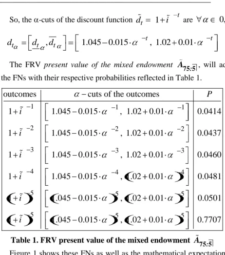
The FRV present value of the mixed endowment A_{75 5}_: , will adopt as values the FNs with their respective probabilities reflected in Table 1.

1 1 1

2 2 2

3 3 3

4 4

outcomes cuts of the outcomes

1 1.045 0.015 , 1.02 0.01 0.0414 1 1.045 0.015 , 1.02 0.01 0.0437 1 1.045 0.015 , 1.02 0.01 0.0460 1 1.045 0.015 , 1.02 0 P i i i i 4 5 5 5 5 5 5 .01 0.0481 1 1.045 0.015 , 1.02 0.01 0.0501 1 1.045 0.015 , 1.02 0.01 0.7707 i i

Table 1. FRV present value of the mixed endowment A75 5:

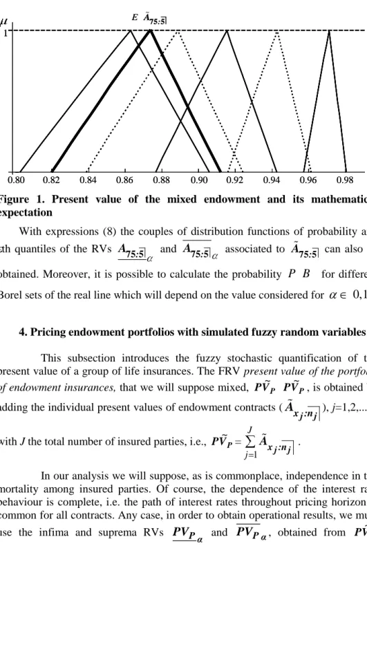
Figure 1 shows these FNs as well as the mathematical expectation of the FRV, whose - cuts are calculated as indicated in (6). Using (7) the standard deviation of this FRV is D A_{75 5}_: 0.0296.

(13)

__________________________________________________________

Figure 1. Present value of the mixed endowment and its mathematical expectation

With expressions (8) the couples of distribution functions of probability and th quantiles of the RVs A_{75 5}_: and A_{75 5}_: associated to

:

A_{75 5} can also be obtained. Moreover, it is possible to calculate the probability

P B

for different Borel sets of the real line which will depend on the value considered for

0,1

.

4. Pricing endowment portfolios with simulated fuzzy random variables

This subsection introduces the fuzzy stochastic quantification of the present value of a group of life insurances. The FRV present value of the portfolio of endowment insurances, that we will suppose mixed, PV~_P PV~_P, is obtained by adding the individual present values of endowment contracts (

j j

x :n

A

), j=1,2,...,J, with J the total number of insured parties, i.e., PV~_P=

1 J

j x :nj j

A .

In our analysis we will suppose, as is commonplace, independence in the mortality among insured parties. Of course, the dependence of the interest rate behaviour is complete, i.e. the path of interest rates throughout pricing horizon is common for all contracts. Any case, in order to obtain operational results, we must use the infima and suprema RVs PV_{P α} and PV_P_α, obtained from PV~_P

E A_{75 5}_: 0.80 0.82 0.84 0.86 0.88 0.90 0.92 0.94 0.96 0.98 1 1 E A_{75 5}_: 0.80 0.82 0.84 0.86 0.88 0.90 0.92 0.94 0.96 0.98 1 1

(14)

Jorge De Andrés-Sánchez, Laura González-Vila Puchades __________________________________________________________

0,1

, defined as PV_{P α} 1 j j J j x :n A and PV_P_α= 1 j j J j x :n A where j j x :n

A

and j j x :n

A

are the RVs obtained from the FRV

j j

x :n

A

0,1

, j=1,2,...,J.

The -cuts of the mathematical expectation of PV~_P and its variance are easily obtained using the results of section 3. Specifically, for E PV~_P we obtain,

0,1

: J j n x J j n xj j j j E E E E E 1 | : 1 | : , , ~ A A PV PV V P _P _P _P (9) where j j E A_{x :n} and j j

E A_{x :n} are calculated as depicted in (6a) and (6b).

Regarding the variance:

d V V V j j j jn x n x 1 0 | : | : 2 1 ~ A A V P _P 1 1 1 0

1

2

j j j j J J j j

V

d

x :n x :n

A

(10)

Likewise, in the case of pure endowments, the expectation and variance of the present value of the portfolio can be obtained analogously to (9) and (10).

Now we can determine the fair price of life insurance (net premiums or net premium reserves). On the other hand, fixing stability surpluses for mortality deviations is difficult because the risk can only be quantified with the variance of present value of portfolio. To make an accurate estimate of cost of risk magnitudes it is also necessary to obtain the quantiles of PV~_P using the distribution functions of probability of the infima and suprema RVs PV_{P α} and PV_P_α. However, it is not possible to find an exact analytical expression of these distribution functions.

(15)

__________________________________________________________

Our approximation is based on the random simulation for pricing life insurances in [Pitacco, E., 1986] and [Alegre, A., Claramunt, M.M., 1995]. However, in this case the results of the simulations will be FNs, due to the fuzziness in discount rates, instead crisp values.

To simulate the FRV PV~_P we consider the RVs “moment when the insured amount will be paid”,

j j

n Tx j=1,2,…J. If we suppose a portfolio of pure

endowments, for the jth member of the collective the realizations of

j j n Tx are

{nj,∞} and their probabilities: , 1

j j j j

n px n px . On the other hand, if we suppose a portfolio of mixed endowments the outputs of

j j n Tx are {1,2,...,nj} and their probabilities: _0| ,_1| ,..., _2| , ₁ j j j j j j x x n x n x q q q p .

Subsequently we implement the following steps: Step 1. We will simulate S times the RVs

j j

nTx , j=1,2,…,J. We

suppose that those RVs are stochastically independent. So, the sth simulation of

j j

n Tx , j=1,2,…,J, generates a vector for the moment of payment

1s

,..., ,...,

s s

s j J

T

t

, s=1,2,...,S. Of course, ts_j is the moment when the insured amount will be paid for the jth contract in the sth simulation.

Step 2. For the sth simulation we can now calculate the present value of the endowment for the jth insured, that is the FN _s

j t d , whose -cuts,

0,1

, are _s j t

d

_s

,

_s j j t t

d

.

Step 3. For the sth simulation we calculate the present value of the portfolio, PV~_Ps, by adding the present value of the J policies. It is the FN

J j t s P s j d V P 1 ~ ~

, where the -cuts, PV_Ps , are:

,

s s s P P P

PV

1 1

,

s s j j J J t t j j

d

.

(16)

__________________________________________________________

Notice that in this step the original FRV PV~_P has been approximated by a simulated FRV PV~_P* whose realizations are the FNs

S P s P P P PV PV PV V

P~ 1,~ 1,...,~ ,...,~ with the a probability of occurrence 1

S . This FRV

defines,

0,1

, the infima and suprema RVs PV_{P α}* and PV_P*_α.

Step 4. We describe PV*P from its infima and suprema RVs PV_{P α}* and PV_P*_α.

To do this, the values of these RVs,

0,1

, are ordered increasingly in such a way that the outcomes of PV_P* are

PV

_P(1)

PV

_P(2)

...

( ) ( )

...

PV

_Ps

...

PV

_PS and analogously for PV_P* :

PV

_P(1)

PV

_P(2) …

PV

_P( )s …

PV

_P( )S . With the parentheses we symbolize that the realizations of the RVs are ordered increasingly and not from their position in the simulation. Of course, in this case

PV

_P( )s and

PV

_P( )s may be the extremes of the -cuts of two different realizations of PV~_P* that were obtained in step 3. Now we can obtain,

0,1

, the couple F * y

P V P~ F y F * y P * P PV V P~ , ~ : ) ( ) 1 ( ) ( ) 1 ( ~ 1 1 ,..., 2 , 1 , 0 S P s P s P P PV y S s PV y PV S s PV y F y F * P * P PV V P ) ( ) 1 ( ) ( ) 1 ( ~ 1 1 ,..., 2 , 1 , 0 S P s P s P P PV y S s PV y PV S s PV y F y F * P * P PV V P

From these expressions we obtain the couple of th quatiles * P V P~ Q : ) ( ) ( ~ ~ ~ Q ,Q PV_Ps ,PV_Ps Q * P * P * P PV PV V P for 1 , 1, 2,..., s - s s S S S

(17)

__________________________________________________________ Numerical application

We will analyse the liability of a portfolio comprised of 12 mixed endowments contracts with an insured amount of 1.000 m.u. The insured parties for j=1,2,…,5 are 45 years old whereas for j=6,7,…,12 the insured parties are 55 years old. We price the contracts with the technical basis used in section 3. In both cases the contracts end when the insured is 65 years old (age of retirement). So for people aged xj=45 years, nj=20 and when xj=55 years, nj=10. The possible results

of 20T45 are {1,2,...,19,20} and their probabilities: _{0| 45 1| 45}q , q ,...,_{18| 45 19}q , p₄₅ .

Likewise 10T55 can take {1,2,...,9,10} with the probabilities:

0| 55 1| 55q , q ,...,8| 55 9 55q , p .

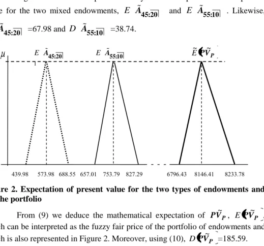
Figure 2 shows the shape of the fuzzy numbers expectation of the present value for the two mixed endowments, E A_45:20 and E A_55:10 . Likewise,

D A_45:20 =67.98 and D A_55:10 =38.74.

Figure 2. Expectation of present value for the two types of endowments and for the portfolio

From (9) we deduce the mathematical expectation of PV~_P, EPV~_P , which can be interpreted as the fuzzy fair price of the portfolio of endowments and which is also represented in Figure 2. Moreover, using (10), D PV~_P =185.59.

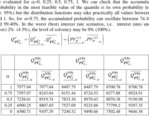
We approximate the FRV PV~_P from S=5000 simulations. Table 2 shows the approximate to its 90th, 95th and 99th quantile couples. Table 3 shows the values of the infima and suprema distribution function evaluated in the mode of the 95th

E A_45:20 E A_55:10 E~PV~_P

439.98 573.98 688.55 657.01 753.79 827.29 6796.43 8146.41 8233.78 1

(18)

__________________________________________________________

quantile in Table 2; i.e. y=8487.79. The infima and suprema distribution function are evaluated for =0, 0.25, 0.5, 0.75, 1. We can check that the accumulated probability in the most feasible value of the quantile is its own probability level (i.e. 95%) but the distribution functions may take practically all values between 0 and 1. So, for =0.75, the accumulated probability can oscillate between 74.10% and 99.40%. In the worst (best) interest rate scenarios, i.e. interest rates under (over) 2% (4.5%), the level of solvency may be 0% (100%).

) ( ) ( ~ ~ ~ Q ,Q PV_Ps ,PV_Ps Q * P * P * P PV PV V P % 90 ~* P V P Q 95~%* P V P Q 99~%* P V P Q % 90 ~* P V P Q 90% ~* P V P Q 95~%* P V P Q 95% ~* P V P Q 99~%* P V P Q 99% ~* P V P Q 1 7977.04 7977.04 8487.79 8487.79 8700.78 8700.78 0.75 7597.07 8243.04 8151.44 8724.53 8377.88 8924.91 0.5 7238.61 8519.74 7833.36 8970.43 8070.38 9156.98 0.25 6900.25 8807.65 7527.09 9225.88 77799.2 9397.35 0 6580.71 9107.29 7240.32 9490.66 7502.48 9646.38

Table 2. Couples of several present value quantiles of the portfolio

y F * P V P~ F * y P V P~ 1 95.00% 95.00% 0.75 74.10% 99.40% 0.5 0.00% 99.90% 0.25 0.00% 1.00% 0 0.00% 1.00%

Table 3. Values of the couple F * y P V

P~ for y=8487.79. 5. Conclusions

Following the developments in [Andrés-Sánchez, J., González-Vila, L., 2012] for life annuities, we model the present value of pure and mixed endowment contracts with FRVs because they allow quantifying their expected price and risk resulting from the uncertainty sources considered.

As several authors mentioned above have done, in this paper we use FNs to quantify uncertain insurance discount rates. We show how the use of FRV not

(19)

__________________________________________________________

only allows the fair price of the policy to be quantified, but also measures for the risk of mortality, both of which are fundamental for fitting surplus over pure premiums or reserves for deviation of mortality. It is important to consider that, to the contrary, “traditional” fuzzy life insurance quantification reduces random cash flows to their expected values, thereby making the risk of mortality difficult to quantify.

We do not want to conclude this section without commenting that the most representative value of a FRV, its mathematical expectation, is a FN. However to state premiums or account reserves in financial statements a crisp quantification of this relevant magnitude is required. For example, in section 4 the expected present value of the portfolio of mixed endowments has a 1-cut equal to 8146.41 whereas its 0-cut is [6796.43, 8233.78]. If we consider that this value quantifies the net reserves of the portfolio it can be understood that “the reserves must be approximately 8146.41 m.u but they may fluctuate between 6796.43 and 8233.78 m.u.” To obtain the definitive value of the magnitude, it must be transformed into a crisp value. To do this a defuzzifying method (see [Zhao and Govind, 1991] for a wide discussion of fuzzy mathematics, and [Cummins and Derrig, 1997] for applications in fuzzy-actuarial analysis) must be applied. Another way of doing this is to consider the fuzzy quantification as a first approximation that allows a margin for the “actuarial subjective judgment” who must use his/her experience to establish the crisp value of the fuzzy estimate.

REFERENCES

[1] Alegre, A., Claramunt, M.M. (1995),Allocation of Solvency Cost in Group Annuities: Actuarial Principles and Cooperative Game Theory;Insurance: Mathematics and Economic, Vol. 17, Pages: 19-34, ISSN: 0167-6687; [2] De Andrés-Sánchez J., González-Vila, L. (2012),Using Fuzzy Random Variables in Life Annuities Pricing; Fuzzy sets and Systems, Vol. 188, Pages: 27-44, ISNN: 0165-0114;

[3] De Andrés-Sánchez J., Terceño, A. (2003), Applications of Fuzzy Regression in Actuarial Analysis ; Journal of Risk and Insurance, Vol. 70, Pages: 665-699, ISNN: 1539-6975;

[4] Betzuen, A., M. Jiménez, Rivas, J.A. (1997),Actuarial Mathematics with Fuzzy Parameters. An application to collective pension plans ;Fuzzy Economic Review, Vol. 2, Pages: 47-66, ISNN: 1136-0596;

[5] Boyle, P.P. (1976), Rates of Return as Random Variables ; Journal of Risk and Insurance, Vol. 43, Pages: 693-713, ISNN: 1539-6975;

(20)

__________________________________________________________ [6] Buckley, J.J. (1987), The Fuzzy Mathematics of Finance;Fuzzy Sets and Systems, Vol. 21, Pages: 257-273, ISNN: 0165-0114;

[7] Couso, I., Dubois, D., Montes, S., Sánchez, L. (2007), On Various

Definitions of the Variance of a Fuzzy Random Variable; Proceedings of the 5th International Symposium on Imprecise Probabilities and Their Applications. Prague, Czech Republic;

[8] Cummins, J.D., Derrig, R.A. (1997),Fuzzy Financial Pricing of Property-liability Insurance; North American Actuarial Journal, Vol. 1, Pages: 21-44, ISNN: 1092-0277;

[9] Feng, Y., Hu, L., Shu, H. (2001), The Variance and Covariance of Fuzzy Random Variables and their Applications ; Fuzzy Sets and Systems, Vol. 120, Pages: 487-497, ISNN: 0165-0114;

[10] Gerber, H.U. (1995), Life Insurance Mathematics; Springer-Verlag: Berlin, ISBN

: 0-387-52944-6;

[11] Guangyuan, W., Yue, Z. (1992),The Theory of Fuzzy Stochastic Processes; Fuzzy Sets and Systems, Vol. 51, 1 Pages: 61-178, ISNN: 0165-0114;

[12] Huang, T., Zhao, R., Tang, W. (2009),Risk Model with Fuzzy Random Individual Claim Amount;European Journal of Operational Research, Vol. 192, Pages: 879-890, ISNN: 0377-2217;

[13] Kaufmann, A. (1986),Fuzzy Subsets Applications in O.R. and

Management;Fuzzy set theory and applications, Ed. A. Jones, A. Kaufmann and H.J. Zimmermann, Pages: 257-300. Reidel: Dordrecht. ISBN: 90-277-2262-5; [14] Körner, R. (1997),On the Variance of Fuzzy Random Variables; Fuzzy Sets, Systems, Vol. 92, Pages: 83-93, ISNN: 0165-0114;

[15] Krätschmer, V. (2001),An Unified Approach to Fuzzy Random Variables; Fuzzy Sets and Systems, Vol. 123, Pages: 1-9, ISNN: 0165-0114;

[16] Kruse, R., Meyer, K.D. (1987),Statistics with Vague Data. Reidel: Dordrecht-Boston. ISBN: 90-277-2562-4;

[17] Kwakernaak, H. (1978),Fuzzy Random Variables I: Definitions and Theorems,Information Sciences, Vol. 15, Pages: 1-29, ISNN: 0020-0255; [18] Kwakernaak, H. (1979),Fuzzy Random Variables II: Algorithms and Examples for the Discrete Case; Information Sciences, Vol. 17, Pages: 253-278 ISNN: 0020-0255;

[19] Lemaire, J. (1990),Fuzzy Insurance;Astin Bulletin, Vol. 20, Pages: 33-55.

ISSN: 0515-0361;

[20] Li Calzi, M. (1990),Towards a General Setting for the Fuzzy Mathematics of Finance ; Fuzzy Sets and Systems, Vol. 35, Pages: 265-280, ISNN: 0165-0114; [21] Ostaszewski, K. (1993),An Investigation into Possible Applications of Fuzzy Sets Methods in Actuarial Science; Society of Actuaries: Schaumburg (USA), ISBN: 0-938959-27-1.

(21)

__________________________________________________________

[22] Pitacco, E. (1986),Simulation in Insurance.Insurance and risk theory, Ed. M. Goovaerts, F. De Vylder, and J. Haezendonck, Pages: 43-44. Reidel: Dordrecht, ISBN: 9789027722034;

[23] Puri, M.L., Ralescu, D.A. (1986),Fuzzy Random Variables ;Journal of Mathematical Analysis and Applications, 114, Pages: 409-422. ISNN: 0022-247X; [24] Shapiro, A.F. (2009),Fuzzy Random Variables,Insurance: Mathematics and Economics, Vol. 44, Pages: 307-314, ISSN: 0167-6687;

[25] Zhao, R., Govind, R. (1991), Defuzzification of Fuzzy Intervals;Fuzzy Sets and Systems, Vol. 43, Pages: 45-55, ISNN: 0165-0114;

[26] Zhong, C., Zhou, G. (1987),The Equivalence of Two Definitions of Fuzzy Random Variables ; Proceedings of the 2nd IFSA Congress, Pages: 59-62, Tokyo.

http://www.soa.org/professional-interests/technology/tech-table-manager.aspx.