University of Southern Queensland
Faculty of Engineering and Surveying
Multicore Algorithms for Image
Alignment
A dissertation submitted by
Tristan James Ward
in fulfilment of the requirements of
Courses ENG4111 and ENG4112 Research Project
towards the degree of
Bachelor of Engineering
(
Software
)
ABSTRACT
Parallel processing is an emerging trend in modern computing. Traditional software development paradigms often forsake parallelism in their approach to produce algorithms. Applications developed then effectively relinquish any potential performance benefits gained by using multi–core processing hardware that is presently available. The fundamental idea of using parallel processing is applied to medical research and the results are reported in this dissertation. Advancements in technology within this field have the potential to greatly streamline processing, thereby directing scientific attention back to research.
Advances in medical microscopy are presently being hindered by the substantial time involved with the construction of panoramic imagery. The predominate purpose and focus of the project is to investigate and develop the automation of image alignment and noise reduction to a series of microscopy photographs, using the performance advantages of multiple processor cores. The output of the algorithms is the formation of a single microscopic panoramic image.
University of Southern Queensland
Faculty of Engineering and Surveying
ENG4111 and ENG4112 Research Project
Limitations of Use
The Council of the University of Southern Queensland, its Faculty of Engineering and Surveying, and the staff of the University of Southern Queensland, do not accept any responsibility for the truth, accuracy or completeness of material contained within or associated with this dissertation.
Persons using all or any part of this material do so at their own risk, and not at the risk of the Council of the University of Southern Queensland, its Faculty of Engineering and Surveying or the staff of the University of Southern Queensland.
This dissertation reports an educational exercise and has no purpose or validity beyond this exercise. The sole purpose of the course pair entitled “Research Project” is to contribute to the overall education within the student’s chosen degree program. This document, the associated hardware, software, drawings, and other material set out in the associated appendices should not be used for any other purpose: if they are so used, it is entirely at the risk of the user.
Prof Frank Bullen
Dean
CERTIFICATION
I certify that the ideas, designs and experimental work, results, analyses and conclusions set out in this dissertation are entirely my own effort, except where otherwise indicated and acknowledged.
I further certify that the work is original and has not been previously submitted for assessment in any other course or institution, except where specifically stated.
Tristan James Ward
Student Number 0050086907
_________________________________
Signature
ACKNOWLEDGEMENTS
I would like to thank my supervisor Dr. John Leis for his ongoing support, expertise, guidance and patience throughout the duration of this project. Without his assistance and direction, this project would not have come to fruition. I would also like to acknowledge the unconditional love and support of my family over this time. It was much appreciated.
T. WARD
CONTENTS
ABSTRACT ... ii
CERTIFICATION ... iv
ACKNOWLEDGEMENTS ... v
LIST OF FIGURES ... ix
LIST OF TABLES ... x
CHAPTER 1 INTRODUCTION ... 1
1.1 Context ... 2
1.2 Current System ... 3
1.3 Design Aims ... 4
1.4 Project Objectives ... 5
CHAPTER 2 LITERATURE REVIEW ... 6
2.1 Existing Technologies ... 6
2.2 Multi–COre Design ... 10
2.3 Image Stitching Algorithms ... 11
2.4 Noise reduction algorithms ... 13
2.5 Coding Style ... 15
2.6 File Formats ... 17
CHAPTER 3 METHODOLOGY ... 20
3.1 Research and Design ... 20
3.2 Programming Language ... 21
3.3 Hardware and Software Platforms ... 22
3.4 Performance Testing ... 23
CHAPTER 4 MULTI–CORE COMPUTING ... 25
4.2 Threading ... 29
4.3 Proposed Design ... 30
CHAPTER 5 IMAGE ALIGNMENT ... 33
5.1 Issues and Assumptions ... 34
5.2 Scale–Invariant Feature Transform ... 35
5.3 Correlation ... 37
5.4 The Design ... 39
CHAPTER 6 NOISE REDUCTION ... 44
6.1 Moving Average Filter ... 45
6.2 Median Filter ... 46
6.3 Assumed Design ... 48
CHAPTER 7 PROJECT LIMITATIONS ... 51
7.1 File Formats ... 51
7.2 Image Sequencing ... 52
7.3 File Paths ... 53
7.3 Graphical User Interface Expandability ... 53
7.4 Operating Systems and Compliation ... 54
CHAPTER 8 PERFORMANCE REVIEW ... 56
8.1 Testing Scenario ... 56
8.2 Results ... 59
8.3 Discussion ... 61
CHAPTER 9 CONCLUSIONS ... 67
9.1 Summary of Developments and Findings... 67
9.2 Initial Research Objectives ... 69
9.3 Evaluation of The Algorithms ... 70
9.5 Review Objective ... 71
9.6 Further Work ... 73
LIST OF REFERENCES ... 75
APPENDIX A SPECIFICATIONS ... 83
APPENDIX B CODELISTINGS... 85
B1 Main.c ... 85
B2 alignment.h ... 88
B3 alignment.c ... 89
B4 axis.h ... 101
B5 axis.c ... 102
B6 bmp.h... 104
B7 bmp.c ... 106
B8 boolean.h ... 109
B9 error.h ... 110
B10 error.c ... 111
B11 fileIO.h ... 112
B12 fileIO.c ... 115
B13 noiseReduction.h ... 121
B14 noiseReduction.c ... 122
B15 threads.h... 125
B16 threads.c ... 126
B17 tiff.h ... 130
LIST OF FIGURES
2.1 Different styles of valid programming, with the opening
parenthesis of the C language ... 16 2.2 Graphical distinction between the image file formats,
including: JPEG; BMP; and GIF ... 18 4.1 Block representation of memory usage of two processes ... 28 4.2 Block representation of memory usage of two threads in a single
process ... 29 5.1 Illustration of the mage alignment of two images, showing the
join coordinate ... 33 5.2 Correlation surface plot of the same image, with dimensions
100 × 100 pixels ... 38 5.3 Pseudo code instructions for the calculation of correlation ... 39 5.4 The approach to image alignment for similarity calculation for a
dual core machine ... 40 5.5 Correlation surface plot of different images, with dimensions 100 ×
100 pixels ... 42 6.1 An example of the moving average filter ... 45 6.2 An example of the median filter ... 47 6.3 Demonstration of median filtering for noise reduction on an image
disrupted with ‘Salt ‘n Pepper’ style noise ... 50 7.1 Sample ordering of a 3 X 3 image set, illustrating one possible style
of image referencing for entry on the command line ... 53 8.1 The two images used to stress the project ... 58 8.2 Graph of the result data of testing the project ... 61 8.3 The output panorama after executing the program, using the
LIST OF TABLES
8.1 The hardware specifications used for testing the project ... 57 8.2 Results of executing the project. Time is in seconds to render the
CHAPTER 1
INTRODUCTION
Shortly after the turn of the 21st century, the frequency of single core processors had almost reached the maximum limit (Ramanathan 2006). Instead of increasing performance of a processor by raising the frequency, processor manufacturer giants Intel and AMD sought alternative measures to fulfil the escalating demands. The solution to improve performance was to produce a multi–core processor, to cater for the needs of running multiple process applications seemingly concurrently (Ramanathan 2006). In the last couple of years, multi–core processing hardware has become mainstream and drastically more affordable. With the advent of this hardware advancement, which is evidently here for the indefinite future (Ramanathan 2006), a shift in conventional programming paradigms is required to accommodate the full potential of the hardware.
1.1 CONTEXT
Traditionally, photographic images were produced as hardcopy items, making panorama development difficult and restrictive. Since those times, digital cameras have almost entirely replaced the mature analog film counterparts for the majority of civil uses. Presently digital cameras are relatively inexpensive for resolutions below approximately 20 megapixels. They moreover represent convenience with the ease of transfer of imagery to other digital devices. However whilst still performing the same role, extremely high resolution digital cameras remain excessively expensive and for specific applications, may not exist. This facet represents an impediment for science in general, which often necessitates larger resolutions with specialised equipment to be effective.
Overcoming the exorbitant financial outlay and technical issues are managed equivalently to the domestic solution; by using smaller resolution capture devices and employing software to compensate (Rankov et al. 2005). The process of creating a finely detailed photograph is accomplished with a series of logical steps. Initially a sequence of images is taken at higher magnification using a lower resolution camera. Well constructed imagery will contain a slight overlap on the previous frame. These images are subsequently fed into image creation software, which seeks the overlaps to generate the desired product (Rankov et al. 2005). The result is known as a panorama and should closely resemble the output of high resolution capturing devices.
microscopy is the Australian governmental research group, the Commonwealth Scientific and Industrial Research Organisation (CSIRO).
1.2 CURRENT SYSTEM
Distinctly different hardware and software setups exist between corporations and perhaps between interrelated departments of the same company. The current software that the CSIRO employs is the public domain system ImageJ. ImageJ was developed by Wayne Rasband while employed by the United States National Institutes of Health (NIH) (Collins 2007). Built on the Java runtime environment, the software is platform independent making it choice for many researchers. Since ImageJ furthermore provides mechanisms for expandability, the basic program can be improved by adding specifically designed plug–ins (Collins 2007).
The ImageJ application is not without restrictions however. At the core there are two fundamental limitations of foremost importance affecting the base program. One is that without support, the product does not feature automated generation of panoramas. Consequently manual involvement is required, directing time away from critical research. The second issue faced is that although ImageJ is built on Java for inter–platform compatibility, processing time cannot be accurately estimated due to the approach Java utilises for execution. Limited thread control management and the abstraction of the underlying Java binary code guarantees that the program forfeits capturing the full potential of the hardware and operating system (OS) (Moreira, Midkiff & Gupta 1998).
2011). Image transformation programs by their nature exhibit memory dominating properties, notably having sizeable memory footprints when buffering high resolution imagery (Xiong & Pulli 2010).
When delays occur in graphical user interfaces because of memory or processor overloads, the system appears to the user as unresponsive. This unresponsiveness has been experienced by the microscopy scientists working for the CSIRO. Attempting simple operations such as image alignment becomes a challenging ambition, particularly when it is amalgamated with the waiting of extensive periods for computational intensive activities to be completed.
The choice of the Java language for programming moreover presents a unique problem. Developing in the Java environment has the advantage of portability among different operating systems and hardware configurations (Savitch 2010). The software distributed is compiled into Java binary format; a format necessary to function on the Java runtime environment. In this format, each instruction to be performed is interpreted in real time into native machine binary commands for the system that it is executing on (Savitch 2010). Evidently the real time translation procedure costs valuable processor time. Conversely programming in lower level languages facilitates the maximum processing speed to be achieved, at the cost of requiring recompilation for each system that the application will be used on (Savitch 2010).
1.3 DESIGN AIMS
Essentially the design of the project intends to eliminate the predominate issues associated with the existing system, namely task automation and the proper utilisation of a multi–core system. Ultimately the project seeks to:
II implement the most efficient and proficient alignment and noise reduction approaches, with the intent to decrease processing time.
III output the manufactured panoramic image to a suitable and compatible format for the field of microscopy with minimal information loss.
IV evaluate the performance gains of successive cores on several differing platforms.
1.4 PROJECT OBJECTIVES
Accomplishing the design aims of the project will be realised through the subsequent objectives. The tasks the project will require include:
I research into existing image alignment techniques and how these can be achieved through parallelisation.
II research and critical analysis of current noise removal algorithms and how they can be implemented through parallelisation.
III investigate or otherwise evaluate the expected performance of the different approaches to ascertain the most efficient technique or techniques.
IV design and implementation of a working prototype based on the best processing scheme.
CHAPTER 2
LITERATURE REVIEW
Algorithms for image alignment or noise reduction are not new innovations. Xia & Zhang (2010) acknowledge that composing a panorama from an image set has been explored before, with varying results. Each panoramic algorithm has precise design parameters that are to be considered when it is conceived, whether it be portability, execution speed or accuracy for a specific type of image (Rankov 2005, Szeliski 2006). The concept of multi–core based software development equally is not original. Whilst this concept matured, two differing approaches were proposed to take advantage of the hardware (Hughes & Hughes 2008). It is important to establish the gaps with these two prior developments, to comprehend how the multicore image alignment algorithm can be better applied microscopy.
2.1 EXISTING TECHNOLOGIES
TomoJ is an ImageJ software plugin that allows semi–automated or manual panorama construction, working specifically with photographic imagery from transmission electron tomography (TET). Messaoudii et al. (2007) described TET as:
“... an increasingly common three–dimensional electron microscopy
approach that can provide new insights into the structure of subcellular
components. [TET] fills the gap between high resolution structural methods
(X–ray diffraction or nuclear magnetic resonance) and optical microscopy.”
The statement by Messaoudii et al. gives an insight into the level of work conducted by microscopy researchers at the CSIRO and worldwide. However in documenting the TomoJ plugin, no mention is given of multicore algorithmic design. Without reference to multicore development and with the limitations of ImageJ as presented in the current system section (refer to 1.2), it can be assumed that the software is based on a single core process design. Often software with this capability will widely advertise this feature.
Searching online will result in the discovery of many panorama software applications, not just for computers in general but also the Apple iPhone and Android mobile phone markets. Of these products, two from large corporations are striking, which are the Autodesk Stitcher Unlimited and ArcSoft Panorama Maker Pro products. The interesting detail regarding these products is that they both claim on the boxed feature list to make panoramas with little effort from the user and have hardware optimisation algorithms (Autodesk Stitcher Unlimited 2011, Panorama Maker 5 Pro 2011). These algorithms apparently take advantage of the
logically will decrease the processing time for dedicated hardware (Zhang, Wang & Chen 2010).
Several problems exist with utilising the GPU approach to panorama construction. The first drawback is that the two leading GPU manufacturers, ATI and nVidia, have different programming interfaces to develop with. As cited by Wang et al. (2009), although nVidia has dubbed their technology Compute Unified Device Architecture (CUDA) and ATI has named the hardware ATI Stream, the technologies are similar. Development of GPU functions will be more challenging if two sets of interfaces have to be maintained. Communication of instructions to and from the processor to the GPU is already a complex task (Zhang & Wang & Chen 2010).
A second problem is the assumption that the computer systems utilised for microscopy at the CSRIO and elsewhere have these hardware advancements. Computers can and have been built without a dedicated graphics card for many years (Blythe 2008). There is furthermore no guarantee that a researcher that has a dedicated graphics card will support the CUDA or ATI Stream instruction sets. Yuffe et al. (2011) reveals that Intel has recently released the CPU with an integrated GPU on a single die, codenamed Sandy Bridge. This release introduces other issues, such as developers needing to program for Intel GPU processing in addition to the aforementioned technologies.
As cited by Blythe (2008), another issue with GPU rendering is the data transfer cost. Transferring data between the processor and GPU is an expensive operation and one which increases the overall processing time. Having the GPU close to the CPU on the Intel solution reduces the latency when copying or sharing data. The Intel product makes GPU processing more attractive and should be more feasible in the future, however at the present time it is a new hardware device that needs mainstream adoption.
problem exists where freeware products oriented towards microscopy research or fields of similar nature are not designed to take advantage of multi–core hardware. Eytani & Ur (2004) implies that it is less difficult to implement and maintain singular threaded applications and that developers occasionally use this excuse to avoid spending time on producing multi–core algorithms. It is not uncommon for freeware projects to rely on the support of volunteer developers or donations to continue the expansion and improvement of particular programs (Cubranic & Booth 1999). This is one reason why features that are deemed unessential such as multi– core algorithms are overlooked in freeware software.
Fogel (2006) implies that commercial applications do not have this limitation to the same extent. Businesses have funding which they can spend on paying developer salaries and on pioneering algorithms. The objective of corporations consuming finances is that the expenses are expected to be redeemed in the profits from the sale of the software. This financial backing has a benefit in that the developers are generating income, so the design and implementation of innovative approaches becomes a higher priority than it would otherwise.
2.2 MULTI–CORE DESIGN
Multi–core algorithm design is an integral concept of the project. The anticipated efficiency of present multi–core algorithms undoubtedly is imperative in the potential outcome of the project. The research of Liu et al. (2010) into the performance of multicore hardware systems establishes valuable conclusions. Liu et al. (2010) tested the decrease in processing time relative to the number of hardware processors utilised. Throughout the trials, the algorithm used was the Adaptive Differential Pulse Code Modulation (ADPCM). Yatsuzuka et al. (1998) outlines that ADPCM has widespread usage in public telephone networks for reducing the bandwidth required for both telephone conversations and internet traffic. The results of Liu et al. determined that for large values of data, the performance increase approached the number of cores. This conclusion is understandable in that whilst it is acknowledged that there are processing overheads in the creation of threads and assigning tasks (Silberschatz, Galvin & Gagne 2009), these actions can be diminished when compared to a large overall processing time. When the data is small, the algorithm is not as efficient.
design and more specifically the bus width and memory layout, only the impacts of the hardware on the execution performance are examined.
2.3 IMAGE STITCHING ALGORITHMS
Image stitching is the process of creating a panorama from a set of related images, each with a slight overlap on the next. Xing & Miao (2007) defines image stitching to produce a panorama as:
“... a technique to merge a sequence of images with limited overlapping area
into one blended picture.”
To accomplish this task, Hsieh (2003) describes the generic process of image stitching as:
“... recovering the existing camera motion parameters between [the various]
images and then compositing them together.”
Hsieh (2003) essentially depicts the image stitching process as encompassing two major steps. The first is image registration, which involves determining a point in which to join the photographs either from the features in the images or from the image similarities. Once this coordinate is known, the two photographs can be merged into a single image. The process of finding the join point and merging is then repeated for the number of images to be processed. In advanced algorithms, any distortions, rotations or mild scaling errors are corrected before merging (Szeliski 2006).
combinations of alignment locations is known as a full search. A full search will be the most accurate of searches however it will incur a performance penalty for the significant number of computations required (Chen 1998). The easiest approach for utilising a direct method to image alignment is to shift one image relative to a template image. At intervals the two images are evaluated to calculate the sum of squared differences (SSD) (Szeliski 2006). Over all the movements of the shiftable image, the sought after point is where the SSD function is at a minimum. The median of absolute differences (MAD) is one direct based approach that follows this methodology (Szeliski 2006).
Rankov et al. (2005) disclose Correlation as an example of a direct method that is often used for image alignment and that differs in the approach taken. Although correlation still iterates over all the shiftable locations, it relies on the discovery of the cross product maximum of the two images. The Fourier transform based alignment is another direct method. The Fourier technique operates on the detail that the signal of the shiftable image has the same magnitude as the template image, but with a linearly adjusting phase. This phase can detect the appropriate join coordinate. Szeliski (2006) suggests that the Fourier Transform calculation can additionally be utilised to estimate rotations and scaling differences in the images. However since the Fourier Transform involves the calculation of the correlation algorithm, the Fourier Transform approach is overlooked in this project due to performance concerns.
regularly is applied in systems due to its generic feature detection abilities and library referencing (Hsieh 2003). After the features have been identified in all the images, matching of these features must be performed.
Feature detection algorithms are advantageous over traditional direct methods when there are image acquisition problems. Chen (1998) addresses some of the typical image acquisition related issues including: variations in the light illumination; contrast dissimilarities caused by reflections; movements in the scene between shots; and general lens distortions. Rankov et al. (2005) expressed that image capture issues aside, cross–correlation was the second fastest method they had tested, after the principle axis method which was considerably less accurate. Rankov et al. (2005) subsequently consider correlation as the preferred method. It was discovered that the calculation time of correlation could be reduced by directing the search points in the photographs to anticipated overlapping regions. However this required use of an automatic stage for capture to decrease acquisition differences (Rankov et al. 2005). Since a motorised, automatic stage could not be assumed in practical use with this project, the proposal is not of benefit.
2.4 NOISE REDUCTION ALGORITHMS
confirms some of the factors producing noise, as briefly inspected for image alignment. Srivastava (2010) outlines the factors that induce noise in fluorescence microscopy photographs which include, but are not limited to:
I lens miss–focus. II environmental factors. III instrumental error. IV dark current. V electronic noise.
VI photon limited scientific charge–coupled device (CCD) cameras.
Since image capture recommendations are out of the scope of this project, noise reduction techniques will have to be designed to remove as much noise from the photographic files without reducing clarity. Thangavel, Manavalan & Aroquiaraj (2009) describes numerous approaches to remove noise from images. In most instances, the pixel and its neighbours are assessed to receive the noise reduction result. This set of pixels is known as a window, with the centremost pixel being the one to be replaced (Leis 2011). Each pixel of the image is evaluated, with the window shifting relative to the pixel being considered. Some of the approaches listed by Thangavel, Manavalan & Aroquiaraj (2009) and Leis (2011) include:
I the minimum filter. The lowest value in the window is taken as the selected value for replacement. This darkens the overall image.
II the maximum filter. The highest value in the window is taken as the selected value for replacement. This lightens the overall image.
III the moving average filter. The pixel values in the window are summed and divided by the number of pixels in the window. It is simple to implement, but the output image will be marginally blurry.
IV the median filter. The pixel values in the window are sorted and the centre value selected.
shortcomings in that it: slightly blurs the image; is not robust against impulse noise; and it does not keep the image borders.
VI high boost filter. Low frequency content is removed from the image. The result is that the background detail is improved and the sharpness and brightness of the image is enhanced.
VII trace means filter. The values on the diagonal of the window are summed and divided by the number of pixels on the diagonal. It is not as computationally expensive as the moving average filter.
VIII trace median filter. The values along the diagonal of the window are sorted and the centre value selected. It is not as accurate or computationally expensive as the median filter.
IX the correlation filter. The autocorrelation of an image is computed to remove intense colour variations between pixels, which may correlate to noise.
X the M3 filter. This filter is a hybrid scheme between the moving average and median filters. The maximum of both filters is selected as the value for replacement. High frequency components of the image are preserved, making it suitable for ultrasound imagery.
From the selection of algorithms possible, Thangavel, Manavalan & Aroquiaraj (2009) concluded that the M3 filter was the best on a performance basis. The illustration provided however visually shows the M3 filter loses an arguably significant amount of contrast and clarity. Without this filter, Leis (2011) suggests the median filter as the preferred choice, as it produces fewer artefacts than the moving average filter.
2.5 CODING STYLE
software should be built upon. These qualities reduce the cost of code maintenance and the number of faults associated with the system. Whilst there are various tools to enforce the use of a particular standard in widespread use, no universal coding standard exists. Research by Boogerd & Moonen (2008) reveals a reason that is cited for not using the software is that the developers are bombarded with warnings of non conformance. Kremenek et al. (2004) tested this claim and observed that every software tool produced false positives when enforcing coding conventions. The number of false positives recorded in the tests by Kremenek et al. ranged from 30 % to 100 %. With no formal standard on how to write applications, the style of the program that is composed is purely related to the opinions and craftsmanship of the author (Fang 2001).
There are numerous programming manuals that endeavour to present guidelines on common and accepted programming styles. Naming conventions, indentations and commenting depth and frequency are just some of the guidelines these manuals will attempt to have developers adhere to. Yet since these are merely guidelines and not rules, a programmer can legitimately disregard such suggestions (Wang et al. 2010). A classic example is where to place the opening { symbol in the C language. Two accepted styles exist, but whichever technique is chosen it is expected that the developer is consistent across all modules. Figure 2.1 shows the differences in style with the parenthesis symbol, both of which are syntactically valid.
(A)
[image:26.595.72.476.596.683.2](B)
Figure 2.1 Different styles of valid programming
Using Figure 2.1 as an example, there are arguments for both versions. The proponents of Figure 2.1 (A) state that one less line of code is used (Mark 2009), whilst supporters of Figure 2.1 (B) claim that the code is more readable since it is not as compressed (Mark 2009). In either case, the convention chosen by the developer should be reflected throughout the differing type constructs and the work in general for consistency and professional appearance.
2.6 FILE FORMATS
There are numerous file formats presently available for the storage of image data. Work by Bell Laboratories in the late 1940’s began research into compression methods, originally relating to textual communications. Salomon (2002) indicates that there is currently two generic categories for image, video or audio files. The first of these two categories is the lossless compression method, where the data is the same at the decoder as it was originally at the encoder (Salomon 2002). Between the encoder and decoder, the data may be stored in some form of compressed state to reduce the file size or is otherwise stored as raw data. According to Salomon (2002), the second category of compression is the lossy format, whereby the data is different between the encoder and decoder. In an effort to save storage space, some of the information in the original file is lost. The lossy algorithm will remove information, with consideration such that the output of the file visually or audibly appears the same as the original to the user (Xin 2009, Salomon 2002).
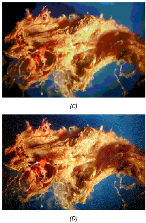
Hannah 1993). Although both BMP and GIF are restricted to 8 bit colour, they handle this limitation in dissimilar approaches as illustrated by Figure 2.2 (CompuServe Incorporated 1990). Another representation of the source image is with the JPEG format, as displayed in Figure 2.2 (B). Neelamani et al. (2006) indicates that JPEG is known as a lossy format and is utilised as such, even though it is acknowledged that lossless JPEG algorithms exist. In the field of microscopy, information loss in photographic files is unacceptable as researchers require as much detail as possible to properly examine samples (Rankov et al. 2005). In this context, lossy file formats are undesirable.
(A)
(C)
[image:29.595.195.441.68.443.2](D)
Figure 2.2 Differences in the output of image file formats (A) Original image, but also
representative of lossless algorithms (B) JPEG Image (C) BMP Image (D) GIF Image.
CHAPTER 3
METHODOLOGY
At its core, this project is about the parallelisation of software tasks to entirely use current hardware. On another level, the project involves the technology used by microscopy researchers and how it can be improved as to direct the focus towards scientific endeavours. Ultimately the automation of tasks and reductions in processing time to produce panoramic imagery represent significant milestones. The first stage of design and development entails background research, followed by selection of certain design parameters.
3.1 RESEARCH AND DESIGN
3.2 PROGRAMMING LANGUAGE
The selection of programming is crucial in the design of the project. Obviously use of higher level languages would decrease the development time due to their simpler syntax, allowing testing to commence more quickly. In various instances this arrangement would be portable amongst different OS environments, as some high level languages are written platform independent (Savitch 2010). A well known and used example of this is Java. The issue with high level languages such as Java is that the native compiled code is often not optimised as assembly (Moreira, Midkiff & Gupta 1998). Execution speed is however forefront to the success of the project. Similarly several high level languages including Java abstract the implementation details from the developer, restricting certain imperative functions such as the capability to fine tune multi–processing aspects.
For best executable performance, the project should be programmed in assembly language (MacKenzie 1988). Unlike high level languages, assembly is dedicated to specific hardware and is not rapidly portable. More crucially, programming in assembly involves extensive knowledge of the intended hardware design layout and substantial time to develop the appropriate program. Since this project is limited by the development duration and it is known that the hardware used may vary, assembly language is not the most suitable.
3.3 HARDWARE AND SOFTWARE PLATFORMS
Originally the project started without any constraints on the hardware or software utilised. As the design and development progressed, real restrictions on the software became apparent. The development of the prototype is restricted to the Microsoft Windows OS by a few Windows dependent Application Programming Interface (API) function calls. Without amendments to these sections of code to be more universal, the OS must be at least Microsoft Windows XP or capable of running surrogate Windows instructions. This prerequisite reduces the software requirements for testing significantly.
Hardware limitations are introduced by the obligation to run the project on Windows compatible and capable systems. For Windows XP, the minimum hardware system requirements are specified by Microsoft (2007):
“● Pentium 233-megahertz (MHz) processor or faster (300 MHz is
recommended)
● At least 64 megabytes (MB) of RAM (128 MB is recommended)
● At least 1.5 gigabytes (GB) of available space on the hard disk
● CD-ROM or DVD-ROM drive
● Keyboard and a Microsoft Mouse or some other compatible pointing
device
● Video adapter and monitor with Super VGA (800 x 600) or higher
resolution ... ”
and larger caches will clearly observe a greater benefit with condensed processing times compared to older hardware.
3.4 PERFORMANCE TESTING
Performance testing is central to the evaluation and analysis of the designed approaches for image alignment and noise reduction. Testing facilitates deductions to be formed regarding the successfulness of the project. The test results of the prototype project application must be recorded in suitable units and obtained with a degree of accuracy to be of value. It is of no benefit to have the technical representation of the results reported in the number of instructions processed, as it is meaningless for assessments in its end use. Considering these rationales, time was selected as the preferred unit for its relevance and understandable comparisons in modern society.
There are numerous methods that could be used to gauge the duration of the image alignment algorithm. Traditionally the counting of the seconds or minutes passed is one approach that could be used without much deliberation. A considerably better approximation is acquired with a stopwatch. A stopwatch could be a mechanical or electronic device. Conveniently Microsoft Windows has a reasonable clock that could be used for timing, since the computer must already be on to execute the program. All of these approaches share a common oversight, in that the tester must be concentrating on the computer until the tests have terminated. Likewise the accuracy of the timing is relative to the human response time, which accumulates an indeterminate amount twice for each test.
deduce conclusions and the human timer might not record adequate differences. Similarly, small deviations in nominal execution such as a simple context switch mid processing would obscure the result. Nevertheless if image sizes or the number of files are set too high, the human timer would be spending large amounts of time waiting. Because of this the timer may not be as responsive to halting the stopwatch at the end of the test, again leading to the inaccuracies as described.
Rectifying the issue of accurate timing is resolved with an inbuilt counter in the application. The time is recorded from the function clock() as an integer representing the number of clocks of the hardware. Comparing the start and end clock values divided by the number of clocks per second gives the time in seconds. After each processing stage and at the conclusion of the program a timed value is printed to the terminal screen. This value is as accurate as practically useable.
CHAPTER 4
MULTI–CORE COMPUTING
Before the advent of the multi–core processor, single core machines dominated with persistently increasing frequencies (Ramanathan 2006). Once the multi–core processor became mainstream, there was a delay in the development of software applications to utilise the hardware entirely. Software continued to be designed on previous generation models and programming languages that only considered the now superseded hardware of the day. This led to sequential programming approaches, much of which is still in existence (Bridges et al. 2007). Designing programs for multi–core processors is not an automated, instinctive approach. Rather careful design strategies contribute to a thoroughly efficient use of the hardware (Bridges et al. 2007). Although some OS environments provide several methods to accomplish multi–tasking, only two generic methods are considered that are reasonably consistent across a diverse range of operating systems. Processes and threads are the aforementioned mechanisms.
4.1 PROCESSES
In terms of computing, a process is defined by the Oxford Dictionary as:
“A series of actions or steps taken in order to achieve a particular end.”
allocated any hardware resources, the instructions form a series of steps that provide a means to solve a problem if followed or run. The transition from the definition of a program to a process follows after the program is loaded in memory, ready for execution.
Considering the implementation in software, an amended classification to the Oxford definition of a process can be altered to accommodate the impact on memory and processors. A software process contains all resources required for operation with an operating system. Examples of the types of resources a process possesses and has control over are: the program counter; hardware processor registers; a stack for temporary data; and a section for dynamic memory provision known as the heap. All of these resources consume system memory and processor time to perform the instructions imbedded in the process. Subsequently, Silberschatz, Galvin and Gagne (2009) informally define the computing process as:
“... a program in execution ... [and which] is an active entity, with a program
counter specifying the next instruction to execute and a set of associated
resources.”
increases relative to the number of processes active. Without otherwise resorting to shared memory or other means to expand the maximum quantity of resources, multi–process applications are an alternative.
The benefits of processes do not come without tradeoffs. The OS accordingly uses the model of processes to manage hardware resource usage appropriately. Without any form of context or relationship between several executing processes, typically the OS will manage processor time by some form of pre–emptive time slicing and will govern system memory by paging infrequently used memory to disk (Silberschatz, Galvin & Gagne 2009). Whilst these forms of hardware management can be effective in many circumstances, they are often inefficient in the context of multi–core programming.
Dependant on the application, a developer is permitted to initiate multiple processes to utilise the various hardware cores (Bridges et al. 2007). A direct disadvantage of using multiple processes to utilise the available hardware is that multiple processes take more computational power. Processes host referencing data that is central for correct OS operation. When the OS decides that the process has had enough time on the hardware, a context switch between multiple processes occurs. When the OS reinstates hardware privileges, data from the presently executing process such as register states have to be copied to storage so that the process can continue execution (Bovet & Cesati 2006). Once complete, the opposite is applied for the process about to begin operation. Data is transferred from storage to the appropriate locations and the process continues from where it was interrupted. Evidently context switching between processes is a timely feat.
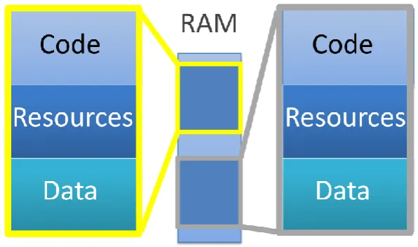
duplicated. Overlooking the situations where the data duplication of multi–process could be tolerated, this type of design is inefficient, producing both slight performance penalties and resource overheads. Figure 4.1 graphically illustrates the issue of memory duplication on a dual core machine which requires two processes.
Figure 4.1 Representation of memory usage of two processes
4.2 THREADING
One of the predominate resources a process includes is that of at least one thread. A thread is defined by Akhter and Roberts (2006) as:
“... a discrete sequence of related instructions that is executed independently
of other instruction sequences.”
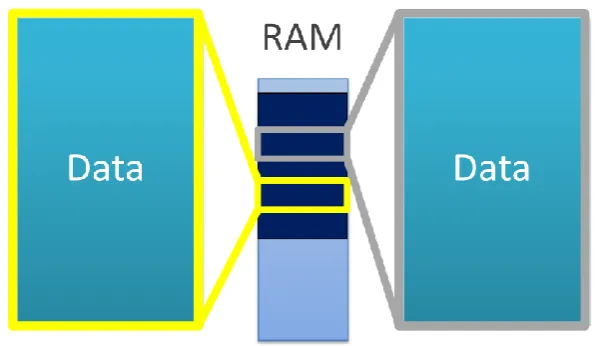
[image:39.595.168.467.514.687.2]Threads are consequently a series of instructions, known as a function, which executes on a hardware unit. The disparity between multiple threads and multiple processes is that threads of the same process inherently share most of the common process–wide resources. Threads are therefore a lighter–weight approach to processes in that threads are less demanding on memory by eliminating the majority of the code and resource duplication observed with processes. The minimum resource requirement for threading includes data items such as the stack (Hughes & Hughes 2008), where local variables and function pointers are situated. Figure 4.2 exhibits the same dual core machine as Figure 4.1, although with multiple threads.
Employing threads in a multi–core system has several benefits. A paramount advantage is that it is more computationally efficient for a changeover between threads than a process context switch (Akhter & Roberts 2006). Threads of the same process share the same distinguishing process attributes, so there is less storage and retrieval of state information when the OS negotiates hardware scheduling. Furthermore threads avert the need for contact between sibling threads to the degree apparent with inter–process communications. Since a thread is perceived to be merely a function, no inter–thread communication is required besides the control of resources and timing. Most common resources are shared by design in threads, so exchange of elements such as global variables are unnecessary (Akhter & Roberts 2006). Savings in both execution and development time and expenses are realistic.
4.3 PROPOSED DESIGN
Conventionally threads are created and destroyed as required, however this induces a performance penalty. Although this method is easier to produce (Lee et al. 2011), each time a thread is created or destroyed an allocation or reclamation of memory and system resources occurs respectively. These transactions consume valuable processor time that could be productively used for processing. Instead the project establishes the threads once at program initialisation. Threads are suspended when in idle state and resumed when there is a task to process.
Generally initialisation of the threads is performed before the threads are used. The threading function in the project prepares the number of threads according to either the number of hardware cores or the input entered as an argument to the process. If present, the input number of threads is capped at the number of hardware cores. Each of the threads is given a dedicated hardware core to operate on, which is unused by any other thread in the process. The rationale is that peak performance is obtained if threads have separate cores and are not in direct contention for equivalent processor resources. A thread will commence by making a call to the OS API to suspend itself, as there are no tasks to process. The API is a set of predefined methods that perform a tested sequence of instructions, without having to develop anything from scratch.
When the point arrives in an algorithm for it to be multi–threaded, a function named assignThreadFunction is called with five arguments. The purpose of this method is to instigate another function to begin operation on one of the threads. The arguments of assignThreadFunction comprise of:
I an integer representing a core on which the proceeding routine should execute on.
II a pointer to a function to process. The method must have a prototype of
void functionName (IMAGE_LIMITS, IMAGE_LIMITS, char*)
A an integer indicative of the image to be operated on.
B a pair of structures that encompass the minimum and maximum coordinates that the processing algorithms can use for boundaries.
IV a pointer to a character array where output data will be stored, if applicable.
Verification that a thread is not formerly processing when it is called and the synchronisation of multiple threads for a particular task involves the analogous concept of a semaphore. Semaphores are an OS level construct that offers a technique of autonomous mutual exclusion (Silberschatz, Galvin & Gagne 2009). Essentially a semaphore is an ordinary variable owned by the OS, which is incremented and decremented atomically. When the value of the semaphore is zero, a process endeavouring to utilise the resource that the semaphore locks must wait until the value of the semaphore is positive. In this project, the first use of the semaphore is to be waited on when trying to task a thread as a precaution. The thread cannot process two items simultaneously; therefore the lock supplies a means of verification that only a singular function can process.
Synchronisation is the second use for the semaphore. Various algorithms require that all threads accomplish their assignment before moving onto the next phase of instructions. This can be illustrated in examples such as averaging across multiple threads. It is evident that if the control thread did not wait until all threads were adequately complete before progressing, an incorrect value for the average could be attained. Even worse, some variables might not be created leading to a segmentation fault. In the project, a dedicated semaphore exists for the number of threads. As each thread is freed of its previous responsibilities, the
waitForAllCores function collects the semaphore of the thread. Once the
CHAPTER 5
IMAGE ALIGNMENT
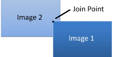
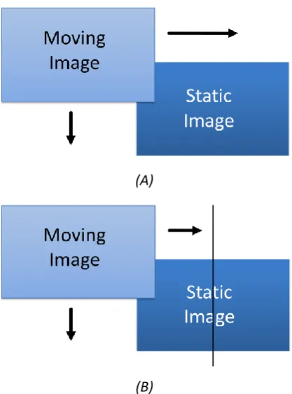
[image:43.595.206.433.510.625.2]Image alignment is the process of engineering a common coordinate system that is shared among a set of interrelated photographs (Hsieh 2003). It is a technique of calculating the similarities in two images and devising a position based system relative to both images. Presently the image alignment algorithms in use consume a tremendous amount of time to complete, as they are a computationally intensive task involving a calculation for nearly every pixel (Chen 1998). In this project, image alignment is employed not purely to formulate a coordinate structure, but to discover alignment points between all of the images. Figure 5.1 shows the point of join with two images. After the points have been resolved, the algorithm must join the images at the predetermined location. Lowering the time the image alignment algorithms take to complete the task can be achieved through multi–processing on a multi–core system.
Figure 5.1 Image alignment of two images showing the join coordinate.
viewpoints. Although this is feasible, in actuality photos that are intended for producing panoramic images are often taken successively, with only a slight variation in the viewpoint. The intent is for no deficiencies to emerge between each shot, though problems arising are inevitable. Alignment of one image to the next is certainly an arduous task, since even small variations in the capture parameters of the image can misguide the alignment position.
5.1 ISSUES AND ASSUMPTIONS
Ideally the panoramic photograph would be captured on a single camera and through a wide angle lens, to negate the time and capital involved in constructing a panorama. Clearly acquiring or obtaining access to high resolution camera technology equipment is not practical in the majority of situations. The next best is to have the simultaneous acquisition of two overlapping photographs, with no differentiation in perspectives or with any form of distortion. Whilst technically this is not impossible, it is just as improbable as the former proposition. Consequently it is acknowledged that some deformation will be present in the images input into the alignment algorithm. The specific application of this project pertaining to image alignment facilitates several assumptions regarding the input files to be made. Image alignment related issues include (Szeliski 2006):
Radial distortion is the curvature of the edges of an image so that a rectangular image warps in a circular profile (Szeliski 2006). Both of these are presumed to be negligible in the images produced by microscopy, as the device is particularly close to the object and the microscope lenses should have low parallax tolerances. No parallax compensation is accounted for in the project.
II the rotations of any image. Unless the images are taken with a tripod or similar apparatus that is absolutely level, some rotations will be introduced. In domestic photography, the rotation might not be enough to be conspicuous and would probably go unnoticed. With medical imagery however, rotations may represent a large issue with the diagnosis. Misaligned images in a panorama could perceivably be misleading to the identification and analysis of the object. Without any prior medical qualification and since image rotations are a per image attribute, applying an autocorrecting rotation to each image is out of the scope of this project.
III the perspective and distortion found in images. Objects that are skewed in the 3D plane can be repaired by affine transformation. Affine transformation is the mathematical properties that allow the vectors of the image in all dimensions to be rotated and skewed as to reproduce the non skewed version. The microscope is nominally calibrated to capture images on a horizontal surface that is parallel to the microscope camera device. Because of this, it is extremely implausible that affine transformations will occur and need to be accounted for.
5.2 SCALE–INVARIANT FEATURE TRANSFORM
detection algorithms available that can depict or outline various details within a photograph. The Oxford Dictionary defines a feature as:
“... a distinctive characteristic of a linguistic unit ... that serves to distinguish
it from others of the same type.”
By this definition, a feature is in essence a point of interest. Whilst being direct in that a feature must be a differentiating component, it is unclear from the description of the exact specifics of what constitutes such a distinction. Due to varied applications where feature detection is utilised (Lowe 1999), many unique forms of feature detection algorithms have been developed. Some such systems include: feature description; edge detection; corner detection; and blob detection. Each algorithm plays a considerable role in the field for which it originates. The SIFT algorithm is part of the set of feature descriptors.
The SIFT algorithm begins by first extracting key points from a collection of reference images (Lowe 1999). These key vector points are stored in a library. When an image is input into the algorithm to have its features identified, the algorithm cycles each pixel generating feature map. The feature map is the vectors of interest which are compared to the library. If a matching candidate is found, the key vectors in the input image are classified and indexed accordingly. The principle benefit of this approach is that overall, detection is invariant with respect to image: scaling; orientation; position; and with minimal effect, noise and slight distortions (Lowe 1999, Hua, Li & Li 2010). Key features are based on an array of vector points and are scrutinised under these attributes. Positive matches discovered are transferred for subsequent analysis which seeks to discard outlier vector objects. The vectors remaining relate to detectable characteristic.
“I Choose an image as referenced one.
II Find the feature matched in the neighboring images.
III Calculate the homography H of the two images.
IV Apply H to warp and project the image 2 to the same coordinate
system as the image 1, and then process image 2 and stitch them
seamlessly.”
A substantial issue with the SIFT approach and all equivalent subsets is that the features present in the images for alignment have not always been identified. The technical field in science of microscopy researches into both existing and undiscovered substances. In the context of this project, the SIFT algorithm is not practical. Maintaining reliable library records to ensure accurate image alignment joins is not convenient, as it leads to microscopy researchers again focusing on technology rather than science. Likewise updating the catalogue of items every time a new object is found would slow progress down in this application.
5.3 CORRELATION
Correlation is a commonly used digital signal processing technique to filter noise from electrical and audio signals (Leis 2011). Noise refers to disturbances in the original signal, such that certain parts of the signal no longer represent the true value. For a number of reasons, signals often gather noise through transmission mediums. Comparing a signal buried in noise with the original will conclude with a negative result. Correlation forms an output waveform based on two inputs, which are the known original signal, and an acquired signal that contains noise (Leis 2011). The correlation algorithm then strives to repair the corrupted signal so that the best waveform that resembles the original is produced. Notably the technique of correlation can be applied to image alignment.
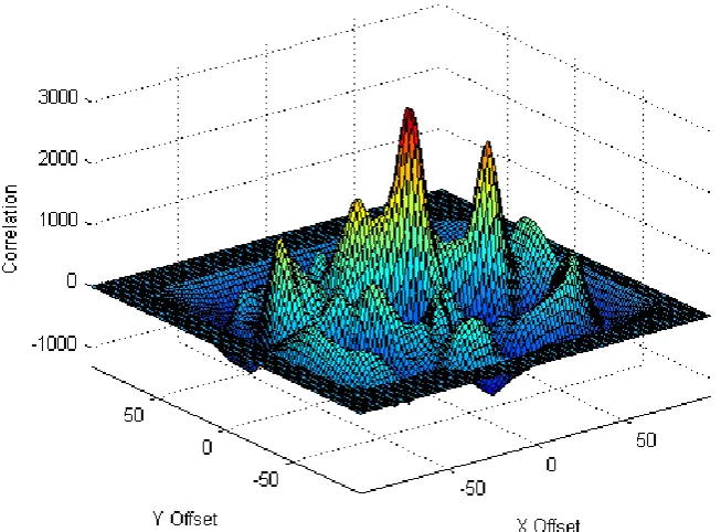
image is shifted relative to the first (Rankov et al. 2005). The shiftable image is incremented from a one pixel overlap in the top left corner of the stationary image, to a one pixel overlap in the bottom right corner of the stationary image. At each increment, the similarity of the overlap of the two images is calculated. It is noteworthy that all computations are only performed on the overlap region of the two images, dubbed the viewport. After all calculations are performed, the algorithm seeks the highest peak in output waveform. The coordinate offset with this highest similarity is selected as the point to join (Rankov et al. 2005). The plot in Figure 5.2 displays the highest peak in the output, which is appropriately positioned at offset (0,0) since the diagram is the correlation of the same image.
Figure 5.2 Surface plot of the correlation of the same image with dimensions 100 100
Figure 5.3 Pseudo code instructions for the calculation of correlation
The calculation of correlation is performed in a number of stages. The sequence for evaluation of the correlation is presented as a codified list of pseudo code instructions in Figure 5.3.
The correlation algorithm has several benefits over SIFT. A significant advantageous factor is that no library scheme is mandatory. The requirement to have existing items in storage for comparisons against in conjunction with maintenance time necessary for library upkeep, increases the prerequisites of the SIFT algorithm. Eliminating these founding prerequisites saves both time and capital. Another advantage of the correlation algorithm is that it is relatively easy to implement in the chosen development environment.
5.4 THE DESIGN
diagrammatically. The looping construct consequently requires modification to utilise a multi–threaded programming procedure.
(A)
[image:50.595.173.382.156.438.2](B)
Figure 5.4 Image alignment approach for similarity calculation
(A) Traditional single–core type (B) Division for a dual core machine.
alignment algorithm. This is in contrast to the many existing implementations that are hardcoded.
The multi–core alignment methodology developed falls short when the algorithm offers two offsets as the join point; one offset for each thread. This issue is overcome by the controlling thread saving all the calculated values from each thread in an array. Once all threads complete the computations, the control thread selects the highest correlation value from the array and uses the corresponding horizontal and vertical offset as the join point. At this point, the offset for this image combination is stored in a separate array. This second array which contains all of the offset values is subsequently normalised, so that one image will start with either a horizontal or vertical offset of zero. Negative offsets will cause corruption when the images are compiled into a single panorama, as the location is used directly for its position in the final image. Undoubtedly image files cannot have negative dimensions. The cycle of calculating similarities on multiple threads, determining the largest and storing the offset result, repeats until all image files are processed.
Figure 5.5 Surface plot of the correlation of different images with dimensions 100 100
pixels.
Figure 5.5 graphically represents the step size problem. When referring to two different images it is common for there to be several crests in the output plot. In any given image, there can only be one peak that is classified by the algorithm as being the highest. If the increment size is set too high in order to save processing time, the genuine highest peak may not be selected as the join point. To rectify this exception, the correlation function repeats itself over the range between the value it has selected as the highest and the neighbours of this selected point. Every increment between both neighbours of the designated peak is calculated with the optimism that any higher peaks could be valid in this range. In the instance of Figure 5.5, if the crest on the right side were to be determined as the highest and the step size sufficiently large, the authentic ultimate peak would be detected during the second iteration.
width of each image, the output image dimensions are ascertained. Local memory is allocated according to this size. Utilising the same approach used for division of the image alignment task, the activities of image compilation and the transfer of local data is multi–processed. The output image data is transferred to a location of choice; namely the output structure in memory that is written to disk.
CHAPTER 6
NOISE REDUCTION
Noise refers to the amount of errors or imperfections that are enclosed in an image compared to what is present in the original exposure. Stroebel and Zakia (1993) describe image noise as:
“... random variations, associated with detection and reproduction systems,
that limit the sensitivity of detectors and the fidelity of reproductions ...”
There are numerous reasons why noise exists in images. Some examples of the causes include: dust or particles developed between the camera and the object; light reflections across the lens introducing graininess; or transmission errors altering the intended values (Srivastava 2010). Indeed combinations of these issues are probable which further compounds the incapacity of a photograph to perfectly represent the subject. The challenge of noise reduction ideally is to remove all of these indicated defects and improve clarity in an image.
6.1 MOVING AVERAGE FILTER
The moving average filter is a particularly straightforward noise reduction algorithm. Every pixel of the image is iterated and the mean of the neighbouring pixels are calculated (Mather 2004). Harnessing a 3 3 pixel window size, a single pixel around each extremity of the centremost pixel is summated, including the value of the centremost pixel itself. The centre pixel is the pixel designated for noise reduction. It is subsequently substituted with the mean.
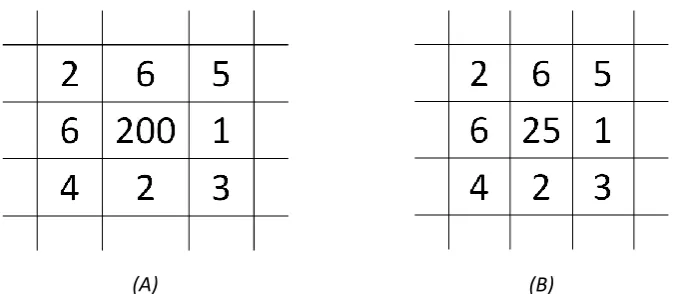
[image:55.595.147.488.292.439.2](A) (B)
Figure 6.1 Moving average filter (A) Original window (B) Window after filtering.
Usage of the moving average filter with a 3 3 pixel window is illustrated with an example in Figure 6.1. It is worth noting that greyscale images are generally represented in files as numbered quantities, therefore this depiction is apt. In this instance, the square for noise reduction is listed as holding the value of 200. Amid the context of the surrounding pixels, it can be perceived that the number 200 is out of perspective. Conveniently, the majority of all noise encountered in this project follows a similar nature to this, with pixel values either being too high or too low for the region. Calculation of the mean results in a slightly more appropriate figure of approximately 25, as visible in Figure 6.1 (B).
significant role in the amount of noise removed. The performance of the filter is restricted to approximately O . Whilst a smaller window size will increase the throughput of the algorithm, too small a window size results in the noise not being thoroughly removed. Conversely, window dimensions that are too large yield poor comparative performance and inferior image clarity. Incidentally, testing seemingly demonstrated that the 3 3 pixel window offers the best ratio of performance to noise removal accuracy.
Window sizing is not the only limiting factor on the effectiveness of the moving average filter. The approach to filtering tends towards instability when the noise is vastly different to the anticipated value. Figure 6.1 displays such a case. It could be supposed that the expected value to be replaced in Figure 6.1 would be no higher than perhaps ten, as apparent by those adjacent to it. Any pixels that are vastly opposing to the predicated will not have noise entirely reduced and will in effect contribute to incongruous values applied in the mean of neighbouring squares. The image thus becomes visually blurry to the viewer (Leis 2011). It is acknowledged that successive revisions of the algorithm will gradually reduce noise, at the expense of the loss of image clarity and perceived blurriness. Likewise the ubiquitous issue arises as with all image filters, which lies in the definition of noise. In this circumstance, it is not clear what actual value should replace the 200 of Figure 6.1, if any. If the algorithm were to be adapted to suit this characteristic, it is very unlikely to be a fitting attribute of all images.
6.2 MEDIAN FILTER
are sorted in ascending order (Thangavel, Manavalan & Aroquiaraj 2009). Sequencing the grid degrades performance moderately to O (Sedgewick 1978). The median filter however is affected by the window sizing for exactly the same rationale as the moving average filter.
[image:57.595.147.482.202.349.2](A) (B)
Figure 6.2 Median filter (A) Original window (B) Window after filtering.
6.3 ASSUMED DESIGN
Design aspects of the noise reduction filter build upon those constructed in the image alignment algorithm (refer to 5.4). Resembling the alignment algorithm, the choice of noise reduction algorithm was the foremost decision. The median filter was opted for as it offers satisfactory performance and of the options, provides the most precision reduction without adversely affecting the overall image clarity. The pixel values that constitute the window are gathered into local memory, with one array for each of the red, green and blue colour channels. The integrated Quicksort algorithm in C is utilised to sort the pixels in ascending order. The median of each of the arrays after sorting is complete and overwrites the existing values held for the image. Therefore alterations are immediate and global for all proceeding operations. Division among threads and consequently cores were conducted identically to the distribution for image alignment, whereby the vertica