The grouping problem in distribution free general linear regression

THE GROUPING PROBLEM IN DISTRIBUTION-FREE GENERAL LINEAR REGRESSION

by

Marthinus J. Pella, Drs.

in the Department of Mathematics

submitted in fulfilment

of the requirements for the degree of Master of Science.

University of Tasmania

Hobart

Marthinus J. Pella

ABSTRACT

ACKNOWLEDGEMENTS

I would like to express my sincere gratitude to Dr. B. M. Brown for supervising this work. His ideas, experience and guidance were invaluable in the preparation of this thesis.

My thanks also go to Mr. Tim Stokes for giving his time in assisting with proof reading and English corrections, and to Mr Glen McPherson,

Mrs. Betty Golding and Mr. Kym Hill for their help in the typing of the manuscript.

I am grateful to the Australian International Development Assistance Bureau for giving an award to allow me to study as a research student at the University of Tasmania.

CONTENTS

ABSTRACT ii

ACKNOWLEDGEMENTS iii

CONTENTS iv

CHAPTER 1. INTRODUCTION 1

CHAPTER 2. SIMPLE LINEAR REGRESSION 6

2.1. Pooled Estimates 6

2.2. Pitman's Asymtotic Relative Efficiency 7

2.3. The Least Squares Method 8

2.4. An Exact DF Method for Slope in

Simple Linear Regression 10

CHAPTER 3. PLANAR REGRESSION 16

3.1. Method of Parameter Elimination 16

3.2. Efficiency Loss Due to Grouping 19

3.4. Minimizing the Loss of Efficiency 21

3.3.1. A Monte Carlo Method

3.3.2. A Search for better neighbour 23

3.3.3. Simulated Annealing Method 25

3.3.4. Computer program 26

3.4. A Numerical Example 32

CHAPTER 4. GENERAL LINEAR REGRESSION 41

4.1. Method of Parameter Elimination 41

4.2. Minimizing the Loss of Efficiency 44

4.3. A Numerical Example 49

CHAPTER 5. DISCUSSION AND CONCLUSION 57

5.1. Discussion 57

5.2. Conclusion 59

APPENDIX 61

CHAPTER 1

INTRODUCTION

Statistical inferences are based only in part upon the observations. An equally important base is formed by prior assumptions about the underlying situation. Even in the simplest cases, there are explicit or implicit assumptions about randomness and independence, about distributional models, perhaps prior distributions for some unknown parameters and so on. Thus we can say briefly that each statistical method is based on special assumptions about the population from which the sample was obtained.

The usual method of solving general linear regression problems is the least squares (LS) method. This method has the nice property of providing best linear unbiased estimates for the unknown parameters; however this method is vulnerable to gross errors in the data and is also inefficient for distributions with heavy tails (e.g., Cauchy—type distribution functions). In such cases we need alternative methods which rely on some broader and weaker assumptions about underlying distributional forms such as symmetry or identical error distributions; namely distribution—free methods.

In simple linear regression (SLR), numerous distribution—free (DF) tests and the corresponding estimates can be developed. The SLR model is

y. = a + fix + c , i = 1, 2, ... , n with {c.} being random errors. Mood and

Brown (1950) have proposed a DF test, based on their median estimates. Parameters a and /3 can be estimated simultaneously from the two equations,

A A A A

median (yi — a — fix.) = 0 for xi < xm , and median (y. — a — fix.) = 0 for x > xM ' where x is the median of x

1' x2' . ' X . The point estimate (a, /3)

i

of slope )3, the median of (n) slopes (y —y )/(x —x ) , 1 < i < j < n , with

2

assumptions that the errors are independent, identically distributed and all x . 1 are distinct. He also obtained corresponding confidence intervals for ig Adichie (1967) considered a class of rank score tests for the hypothesis

a = fi = 0 , with the basic assumption that F(y) = F(y — a — fix) is an absolutely continuous, symmetric distribution with square integrable density function. Moreover his point estimators of /3 required trial and error solutions and also Adichie gave no confidence interval for Sen's (1968) estimate is quite analogous to Theil's (1950) but is based on weaker assumptions and does not require all of the x , x , , x to be distinct. If N is the number of non

12 n

zero differences x — x , (1 < i < j < n) , the proposed point estimator is the median of N slopes (y.—y.)/(x —x ) for which x x . The confidence

ii ii I j

interval for is also obtained in terms of two order statistics of this set of N slopes. Brown and Maritz (1982) made a modification to the LS estimating equations in SLR, leading to exact DF inference about slope. Exact inference for intercept is developed by Maritz (1979), based on work of Theil (1950).

The planar regression model is y = p + ax + /% + = 1, 2, ... n, where { } are random errors, {x . ,z

i} are known and a, 13 are unknown parameters. Suppose is of interest, p and a are nuisance parameters and { e } are identically distributed. Brown and Maritz (1982) showed how a suitable {x . , z} design, coupled with a restricted permutation or restricted

i

3

symmetric errors, and /3 the slope parameter. The Maritz/Theil scheme then is applicable, but since that involves further pairing, the overall problem is one of finding groups of four observations, which through two pairing operations yield one observation distributed symmetrically about

g .

Exact DF methods for the symmetric location parameter problem are then used.

This thesis outlines another approach to exact DF regression methods in the presence of nuisance parameters through grouping of observations to eliminate the nuisance parameters. The number of groups depends on the number of observations and also on the number of independent design variables. For instance in planar regression, the observations are grouped into k groups, where k = [n1/2], the integer part of nil' ; in regression with three independent design variables k = [(n/ 2)1/2]. After grouping and eliminating the nuisance parameters, the model is reduced to simple linear regression form, allowing exact DF methods for slope to be employed.

Of course grouping and reducing the model as described seems to involve a loss of efficiency. A question of interest is the extent of efficiency loss suffered through grouping and reducing the model. How can the groups be chosen to minimize the loss of efficiency? This optimal grouping task is a very difficult combinatorial optimization problem, without convexity or other regular structure leading to efficient unique solution methods. Three methods will be discussed for finding approximate solutions. The methods are : a Monte Carlo

4

has proved to be very successful in diverse Operations Research applications over recent years.

To illustrate how the proposed method in this thesis works, and to demonstrate that the necessary computer programming is relatively straightforward, numerical examples will be given.

To summarize what we have discussed, the

aim of this thesis is to show

how the general linear model (GLM)

y =fi +fix +fix + + fl x +

e

.

, i = 1, 2, ... , n (1.1) o l ii 221 p

where /3., j = 0, 1, , p are unknown parameters, x x

• , x are design

j ii 21 pi

constants, { } are independent errors and identically distributed, with

one of

the fl. (j 0) of interest, can be reduced to the simple linear regression model, through grouping of observations to eliminate the nuisance parameters, allowing exact distribution—free methods for slope in simple linear regression to be employed.

5

CHAPTER 2

SOME BASIC CONCEPTS AND

DOCUMENTED REGRESSION METHODS

This chapter is presented as a basis for the following chapters, so it contains some concepts and documented regression methods which will be used to develop the proposed method. As stated in Chapter 1, the thesis is concerned with efficiency loss due to grouping and reducing the model, so a concept of efficiency is needed. Here Pitman's asymptotic relative efficiency (ARE) will be used and may be obtained by considering the ratio of efficiencies of least squares analyses for grouped and ungrouped cases, so Pitman's ARE and a short summary of4east squares method in the general linear model (GLM) will be discussed. One of the methods for finding the best grouping to minimize the loss of efficiency given in Chapter 3 will use pooling of estimate and variance, so a method of pooling estimates and variance also will be outlined briefly. The last section will outline an exact DF method for slope in SLR (Brown and Maritz, 1982) which will be used after reducing the GLM form to SLR form.

The contents of this chapter are as follows : pooling estimates, Pitman's asymptotic relative efficiency, the least squares method and an exact DF method for slope in SLR.

2.1. Pooled Estimates.

Let 0

1 and 0 2 be two independent estimates of an unkhown parameter 0. ••■

Assume that 0 _{and 02 are unbiased, so for i = 1,2, we have, for minimum} variance

E(0i) —0, and

var(0.) = a.

The pooled estimate 0 of estimators 01 and 02 is

^

^0/1 cr21 92/6r2 2

0 (2.1)

1/U2 + 1/72 / 1 2

and the pooled variance of var(01) and var(02) is

—1 var(e) =

2 1 1

(2.2) a+

a2 1 2

2.2 Pitman's Asymptotic Relative Efficiency.

When two or more statistics are available for testing a given hypothesis, one statistic is considered more efficient if it is more powerful than other statistics, using the same level of significance, at the same fixed alternative. Such a comparison of powers for two statistics based on the same data is usually dependent on the level of significance a, the sample size n (or some measure of sample sizes with several samples), and the fixed alternative at which the powers are compared. In order to define a suitable measure of efficiency, an alternative approach is adopted comparing the corresponding sample sizes necessary to attain an equal power, say 13, at the same alternative for two tests using the same level a. A limit argument is usually needed for this measure to be independent of particular values

8

a, n; furthermore one needs to use then a sequence of alternatives converging to the null hypothesis at a suitable rate in order to come up with a meaningful definition.

Pitman (1979) defines asymptotic relative efficiency as follows :

Let 0₁ and 0 be two unbiased estimators of an unknown parameter 0, and n

2

the sample size. For n —> 00 , the efficiency of 01 relative to 02 is

urnvar(0 ) 1 e =

n —> var(0 )

2

(2.3)

where var(0 ) and var(0 ) are the variance of 01 and 0 respectively.

1 2 2

2.3: The Least Squares Method.

This section will give a short summary of the least squares method in the GLM. If the GLM equation (1.1) is written in a matrix notation, we have

= xg c (2.4)

where Y._{T = (yi, Y2, Y )}

'

(

fi

) , cis = (c c c ) and 0 1 12 ' n

lx X X 11 12 IP

lx x X

21 22 2p

x

=

9

The least squares assumptions for the error terms are

(i) } are random variables with mean zero and variance 02 (unknown) , that is E(c ) = 0 , var(c ) =

02.

(ii) {c } are uncorrelated, that is if i # j, cov(c.,c.) = 0. .1

(iii) { c.} are normally distributed random variables, that is c•- N(0,a2 ).

The problem is solved by minimizing the sum of squares

S= xg)T(

x

—

_xg)

= — 2gTXTy + gTXTxg

by differentiating S with respect to # , equating to zero, so obtaining the normal equations

xTxg )(T

x

_(2.5)

We assume that X has full rank (p+1) , so

g

(the LS estimate of

/) is

g= (xTx)

-1

xT

x

(2.6)

From the least squares assumption E(ci) = unbiased estimate of

g,

and by assumptions or 1 according to whether i # j or i = j , we get

0 , it can be shown that

g

is an cov(c., c.) = a

-

2

, where is

0

1 j ij ij

e i.e. the covariance matrix of the elements of

g

, so that var()3. ) = a ,

1-1

i = 1, 2, ... , (p+1) , where laiil are diagonal elements of the matrix (XTX)-1.

2.4 An Exact Distribution—Free Method i for Slope in Simple Linear Regression.

Brown and Maritz (1982) made a modification to the least squares estimating equations, leading to exact distribution—free inference for slope. Instead of the least squares assumptions (i), (ii), and (iii) in Section 2.3., their method relies merely on two broader and weaker assumptions about underlying distributional forms, i.e. independent and identically distributed errors. These assumptions enable the basic permutation argument to be applied to obtain an exact permutation procedure for the slope parameter.

The model used is

y =

a +

fix + c , i = 1,

2, ... , n where a,

g

are 1

unknown constants, {x.} are design constants, { .} are independent errors, identically distributed. The least squares estimating equations

r = 0 1=1 and

x r =0 i=i

where r. = y — a — , are modified to the general form

1b(r) = 0 1.1

and (2.8)

h(x.)///(r.) = 0

1=1

11

Both h and '0 should preserve the original orderings of {x.} and

Ir.}.

In addition, 0 should be suitably centred so that the first equation of (2.8) provides consistent estimates of ct when )5' is known. Though the approach is general, the various exact tests and confidence intervals are worked out in detail only for three specific cases of the general residual transformation 0 ; the cases considered are .0 equal to sign, rank and 7/)(x) = x itself. Modified designs of h are used throughout and also for h = sign, rank and identity.

Of course, as a consequence of the transformation described, an efficiency loss will be involved. The asymptotic efficiency of the estimate of slope relative to least squares is

(2.9)

where p is the limit correlation coefficient between {h(x.)} and {xi}, and elk is an efficiency factor associated with 0.

A different choice of h and 7,1) will give different efficiency loss results. For each of the choices of 0 given, the associated procedures are less than optimal under at least one criterion; the choice sign suffers loss of efficiency, the choice rank is difficult to compute, and the choice of identity is not robust (the least squares choice).

12

choices of h and tp will be needed. For illustrative purposes the choices h(x) = x and OW = rank (r) will be used and will be outlined in this section.

Inference about only slope )3 is based on the estimating equations (2.8), for h(x) = x, 0(r.) = rank(r.) — (n+1)/2 , and because rank(r.) is independent of a

S(fi) =

xi{rank(yi — )3xi) — (n+1)/21. (2.10)

S is a monotone function of )3 which decreases only in downward jumps at certain

13 values, i.e. at = )3. = (y. — y.)/(x — x.) for all pairs i, j.

We now discuss the usual statistical inference problems, i.e. the problem of point estimation, confidence intervals and hypothesis testing.

Suppose )3_o is the true value of the slope /3. The estimated value of fl_o is the weighted median of )3.. with weights Ix. —x.1 for all pairs i, j , so

13 1 j

a

. Weighted median Y- Y 'o Weights Ix.-x I x_{1 j} . — x.

1

(2.11)

where )3_o is the estimate value of )3_o.

Tests H_o : 48 = )3_o are rejected for large or small values of _S(fl). Because of the assumption of identical error distributions, the exact null distribution of

T = S(/3

o) + n(n+1)X12 is enumerated by calculating all the values i x =1 p , where

p , p , p is a permutation of 1, 2, ... , n. All n! such values are equi—probable, 12

n

and

(/). T))2

= 0(1) (2.13) 13

In most cases it is convenient to use the normal approximation. According to Wald and Wolfowitz (1944), if the sequences (x i, x2, , x.) and (PI, P2, P.)

satisfy condition W , that is for all integral r > 2

(x . i)r

= 0(1)

r/2 (2.12)

(x .

3

-

02

then the distribution of

r = T —E(T) Var(T)

approaches the normal distribution with mean 0 and variance 1 as n —> co , where E(T) = n i , Var(T) = (S.Spp)/(n-1) ,

= (

xj)/n , 15 = ( irr1 p i) n , S _i (x — 302 and S

p = (p — 15)2 , and therefore the approximate

XX •_{=1 i} p i=1

distribution of T is

T x.p. - N i=1

S S nip, xx PP)

14

Because (pi, p2 , ,

pn)

is a permutation of (1, 2, ... , n) , the condition

(2.13) is satisfied, so whether (2.14) is satisfied or not merely depends on the condition (2.12).

If the rank scores are chosen centred, that is E

p . =

0 , or

p . =i—

(n+1)/2,

we have

S S

T= x .p .

-

N(0 xx

i1 and

p T

o

)2 =

n(n

2

-1)

PP

12 •

Thus the null distribution of T is

N(0,n(n+1 )

12 xx (2.15)

For confidence intervals, the behaviour of S has to be examined. From (2.10) we obtain

and

S(—co) = x . 1 rank(x . ) — (n+1)/2

1

(2.16)

Thus

S(co) = V _L x.1 (n+1) — rank(x) — (n+1)/2 1 i=1

= — X. rank(x.) — (n+1)/2 1 i=1

(2.17) 15

S decreases only in downwards jumps of size Ix —x I at # = #. for all pairs• j. From (2.16) and (2.17) we see that S(+00) = — S(—o) , so the structure of S may therefore be enumerated systematically; the confidence intervals for the slope # must have some

p

as their end points, and the approximate confidence level of

ii

CHAPTER 3

PLANAR REGRESSION

This chapter outlines the proposed method of solving the planar regression problems when only one of the slope parameters is of interest. The basic steps are as follows. Firstly, eliminate the other slope parameter through grouping of observations such that the planar regression can be reduced to SLR form; the group is chosen to approximately minimize the efficiency loss. Secondly, estimate or test the slope of interest by using an exact distribution—free method for slope in SLR.

This chapter is concerned with the first step and outlines the method of parameter elimination, the method of calculating the efficiency loss, the method of minimizing efficiency loss, the computer programs and a numerical example to illustrate how the method works.

3.1. Method of Parameter Elimination

In planar regression, the usual model for fitting a straight line to data is :

y. = p+ ax. + Oz.+

i, i = 1, 2, ... ,n (3.1)

where n is the number of observations, {x., z.} are design constants, { e.} are independent errors, identically distributed with finite variance, and p, a, # are unknown parameters. Suppose # is of interest, and that p and a are nuisance parameters.

17

There are many possibilities for grouping of observations to eliminate the parameter a and reduce the equation (3.1) to SLR form, but this section outlines just one simple method of grouping. Other methods of grouping will be discussed later (see Chapter 5). The method is said to be simple because it is straightforward compared with other methods; moreover after reducing the model to simple linear regression form, the slope parameter of interest can be estimated or tested directly by employing an exact DF method for slope in simple linear regression.

To eliminate the parameter a , the observations are placed into k groups where

k= [n1/9.

y

the integer part of n1 /2. Let A, A, , A be constants, and for i = 1, 2, ... , 1 2 k

k, define

=Ay j j+ko = A _o . + a A .x. A z

=1 j., j+k(i-1) j=1 i- )

Ae f . (3.2) j . j ., +kki-1)

Suppose that {A } are chosen so that for all i = 1, 2, ... , k ,

Ax

j I

=

constant , x* say.

Then from (3.2) and (3.3)

y* A* + gz* + e*

where y*. = E Ay. f , p* = + aoc* , c= A , z* =E Az • f

1 j=1 j+kki-1) j=1 j i j=1 j j+kk1-1J

and

e*

= Xe f . \. The equation (3.4) is of SLR form because len are

j=1 j j+kki-1)

independent, identically distributed, and so can be treated by exact DF methods.

How can {A.} be chosen to assume that (3.3) holds? Let AT = (A , A , , A ) and a kxk matrix X be such that (X) = x

1 2 k i,j j+k(i-1) •

We need to find A to satisfy (3.3) , i.e so that

X A = x* 1

where 1T = (1, 1, ... ,1) . Since the value of x* is immaterial, the choice

A = X-1 1 (3.5)

will always suffice. That is, the row—sums of X-1 provide the multipliers {A . }.

The k pairs of values le, yn for the SLR model (3.4) can be I

calculated more easily using a matrix notation. Let k x k matrices Z and Y be such that (Z) = z \ and (Y) = y f N . If z*T = Z*, ,z*)) 2 k

j+kki-1) i,j j+kki-1)

Of course, X needs to be non—singular, and only non—singular X should be accepted in the random search methods soon to be described. See also Brown, B.M. and Pella, M.J. (1.991), The grouping problem in distribution—free planar regression, Austral. J. Statist. 33, to appear.

18

and y*T = (y*, y*, ,y*) then

1 2 k

19

(3.6)

We have reduced the planar regression (3.1) with n observations to SLR equations (3.4) with k observations.

3.2. Efficiency Loss due to Grouping.

As stated in Chapter 1, grouping and reducing a model will result in, a loss of efficiency. The extent of efficiency loss thereby suffered is a question of natural interest.

By an analysis similar to that in Brown (1985) , it can be shown that the asymptotic efficiency of exact DF methods applied after grouping is

e_G.e_{DF '} where e is the characteristic efficiency of the particular DF DF

method used (for example as in the symmetric location problem or simple linear regression), and where eG is a factor attributable to grouping. The factor e G is of interest here, and it may be obtained by considering the ratio of efficiencies of least—squares analyses for grouped and ungrouped cases.

Such a ratio of efficiencies is just a ratio of variances of estimates of )3 (see Section 2.2). If equation (3.1) is written in a matrix form, we have

X Z 1 1 lx Z

2 2 A =

x Z

n_

i

r

= (Y Y --- Y ) , °T = (ii, a, /3) and err = (E , C , ... , c ) . Suppose that

l' 2" n — _,. 1 2 n

LS assumptions are valid, and if # LS is the ungrouped LS estimate of 0 , then from (2.7)

var(ks) = a {(ATA)'I„ , (3.7)

where cr2 is the observational error variance. After grouping

y* = A* 0* + c*

where eT = (y*, _{Y* , ••• Y:)}

2

1 z* 1 z*

A* = 2

0*T = (p*, #) and c*T = (e* c* (*). The LS assumptions also hold for the — 2" k

GLS is the least squares estimate of # after grouping, then from (2.7) fi

var(fiGis) a*2{(A*TA*)-1} 22 (3.8)

where a*2 = var(e *) = o-2 E \2 • Thus from (2.3), (3.7) and (3.8) we =1

obtain

e_G =

var(flGLs) A2. A * TA*r i = 1

The formula (3.9) is the asymtotic efficiency of estimates of slope for the grouped LS relative to ungrouped LS.

3.3. Minimizing the Loss of Efficiency

To maximize the grouping efficiency e G , it follows from (3.9) that Var(#_GLS) must be minimized, i.e. groups are to be chosen to minimize

k )2

=

{(A*TA*)-1} A2 = j1 22

i=1

k z*2 — ( z* =1

)2

(3.10) 21

var(fiLs ) {(ATA)

J _(3.9)

22

22

efficient unique solution methods. Three methods for finding approximate solutions will be described.

(i) A Monte Carlo method, estimating the probability of having the optimal solution, suitable for small or medium—sized designs;

(ii) a search method which seeks improved neighbours of any current solution, which is easy to program and implement but which can get stuck in local optima; and

(iii) a general technique known as simulated annealing, of great recent popularity in operations research circles.

The two large—sample methods (ii) and (iii) will then be illustrated and compared via an example.

3.3.1. A Monte Carlo Method.

When n is not too large, it can be surprisingly efficient just to generate completely random groupings, evaluate e G for each, and repeat a large number (say N) times. Although it may appear that there are a large number (n!) of possible groupings, many will share the same value of eG , as can be observed by noting that e G is unchanged by swapping rows and/or columns in the matrices X, Z and Y. Therefore if N is large, the probability that the current maximum e_G is in fact the overall maximum can be surprisingly high.

23

much larger. Count the number of times a value e G occurs which was among the initial set of m values.

Let U be the number of such occurences, so that U - Bi(N, m/M) , where M is the total possible number of different e_G values. When U is observed, a confidence interval for m/M and hence for M may be evaluated. Possibly the use of approximations Binomial —> Poisson > Normal is the easiest path to take in getting the confidence interval.

To illustrate, for the design with n = 9 points (using 9 observations selected randomly from the data of the numerical example of Section 3.4), an initial set of m = 83 distinct e values followed by N = 40,000 further random groupings gave U = u = 459 . The resulting approximate 95 % confidence interval for the Poisson parameter mN/M is (418.89 , 502.96) and the corresponding interval for M is (6601 , 7926).

What then is the probability that among 40,000 values of e G , the overall maximum is already present? Taking a conservatively large estimate of M as 8,000 , the probability of missing the maximum is e-5 = 0.0067; the calculations are as for the famous " birthdays paradox " . Thus in this case we can be over 99 % certain of having already found the overall solution.

3.3.2. A search for better neighbours.

24

A simple neighbours search is to start with any randomly chosen grouping, and generate a neighbouring grouping by interchanging a randomly chosen pair. Evaluate eG for the new grouping, and move to the new grouping if the e value exceeds that for the original grouping. Keep re—generating random pairs and moving to better neighbours indefinitely, or until the procedure appears to terminate at a local maximum with no better neighbours. Repeat the whole procedure several times to see if improved finishing groupings can be obtained.

Because every grouping has n(n-1)/ 2 neighbours, it can be more efficient to generate s neighbours at random at each step, where s is a fixed integer possibly greater than 1 . Choose the neighbour with best value of eG and move to it if the new e exceeds the old. For s > 1, this refinement can lead to more rapid improvement.

A variation of the neighbour search is to divide the data into two (or more) separate sets, and carry out the grouping operation separately within each set. Each set yields an independent estimate of , say /31 and )62 , with different expressions var(fli) and var(fi ) . The final combined estimate will

2

use weight proportional to (variance)-1 (see Section 2.1), and the final expression for grouped efficiency is

eG "TA)-1133 1[{(A*TA*)-1}22 Aj2 ]-1 (3.11)

where refers to a sum over the two (or more) sets.

25

All these variations on the neighbour search theme end at local maxima which, while usually having good efficiency, might not be the overall optimum.

3.3.3. Simulated annealing.

The method of simulated annealing stems from Kirkpatrick et. al (1983), who applied to general optimization problems a method of Metropolis et. al (1953), which mimicked the passage to crystalline states of cooling high temperature material. The technique has proved to be very succsessful in diverse Operation Research applications over recent years.

When applied to the optimal—grouping problem, the method is as follows.

(i) Generate a new grouping G1 and evaluate its grouped efficiency eGi . The new grouping can be generated in any fashion, either totally at random or by some interchanges of pairs within the existing grouping Go . However, generating totally random new groupings would be computationally wasteful, and some method based on small changes to Go is preferable.

(ii) Accept G1 if eGi > eGo . Otherwise, accept G1 with probability

p = exp { — (eGo — eGi)/ T)} , (3.12)

where T is a " temperature " parameter which is decreased in some slow manner during the course of iterations.

26

Note that worse G1 can be accepted, with a relatively high probability at early stages when T is high, but with much lower probability later on. Thus G1 can escape from local maxima, but it is more difficult to escape from later local maxima which are more likely to be " close" to the overall maxima.

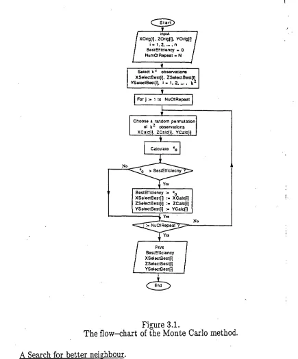
3.3.4. Computer Programs.

This section outlines just the basic steps of the computer programs for finding an approximation of the best grouping, whereas the complete program can be seen in Appendix 5.

Because only k 2 observations of the n observations available are used for estimating the parameter of interest, firstly we have to choose the k 2 observations from the n observations randomly. Our aim is to allocate the k 2 observations into k groups such that e G will be maximum; however, to simplify the flow—charts we just need to find an order of the k2 observations, because when we allocate the k2 observations into k groups, the first k observations becomes the members of the first group, the second k observations becomes the members of the second group and so on. So our aim now is to find an ordering of the k 2 observations which minimizes the loss of efficiency.

27

complete flow—chart will be very complicated, so to simplify the flow—charts, here we just show how to get the approximation of the best order of data without describing the flow—chart of the procedures of choosing the k2 observations, calculating eG , and so on. Those procedures can be seen directly in the computer programs.

Monte Carlo Method.

The arrays used to store the data are as follows :

(i). X0rig[i], ZOrig[i], YOrig[i], i = 1, 2, ... , n , are used to store the original ordering of the n observations.

(ii). XSelectBest[i], ZSelectBest[i], YSelectBest[i], i = 1, 2, ... , k 2 are first used to store the k2 observations selected, and later for keeping an ordering of the data which gives improved efficiency.

(iii). XCalc[i], ZCalc[i], YCalc[i] are used to store an ordering of the data used for calculating e ₀ G •

Some other variables used in the flow—chart are: (i) BestEfficiency is used to store the best eG so far.

(ii) Nu0fRepeat is the number of repeats of the procedure of calculating e G to get an approximation of the best efficiency.

BestEfficiency :. XSelectBest(i] XCalc[1] ZSelectBest[i] 2Calcjil YSelectBest[i] YCalc[ij

Yes

Choose a random permutation of k2 observations

XCalcfil, ZCalcfil, YCalcjil

NuOf Repeat No

I X0rigfij. 20rig(i], YOrig[i] input

BestEfficiency - 0 NumaRepeat - N

Select k` observations XSelectBest[i], ZSelect8est[11 YSelectBest[i], I . I, 2, ... kh

I

For j to NuOtRepeat

Yes

Print BestEfficiency XSelectBest[il 2Selec:Best[i] YSelectBest(i]

Figure 3.1.

The flow—chart of the Monte Carlo method.

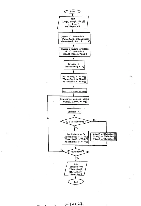
A Search for better neighbour.

The arrays needed to store the data are the same as the Monte Carlo

method, except that XSelectBest[i], ZSelectBest[i] and YSelectBest[i] have a

slightly different meaning, in that the arrays are first used to store the k2

observations selected, and then for storing a neighbour which gives improved

efficiency. The variables BestEfficiency and Nu0fRepeat have the same

meaning as for the Monte Carlo Method. The flow—chart is as follows :

[image:34.562.74.509.53.578.2]

nterchange elements within XCalc[i). ZCalc[i], YCalc[i)

vi

Calculate e0

BestEliciency es XCalc[il XSelectaest[i] XSelectBest[il XCalc[il 2Calc[i] ZSelectSestri) ZSelectSest[i] ZCalc(i) YCalc(i) YSelectEiest[i) YSelect3est[f] YCalc(i)

No

i NuOtRepeat ? C.— Start

V

1

input X0rig[1]. ZOng[71, YOrig[11

Nuallepeat - N

choose le ooservations XSelectBest[i). ZSelectBest[ill

YSelectEtestri). i . 1. 2. -.. k

Choose a rancom permutation of kz ooservations XCalc[i). nalc[11, YCalc[i]

Calculate es BestErliciency eG

XSelectBest[q XCalc[i] ZSelectBestD) ZCalc[i] YSelectSesqg YCalcD]

For I 1 to Nu0fReoeal

V Print Best Elf iciency XSelectBest[i] ZSelectSest[i] YSelectlilestM

Figure 3.2.

The flow—chart of a search for better neighbour

[image:35.562.73.522.63.720.2]

30

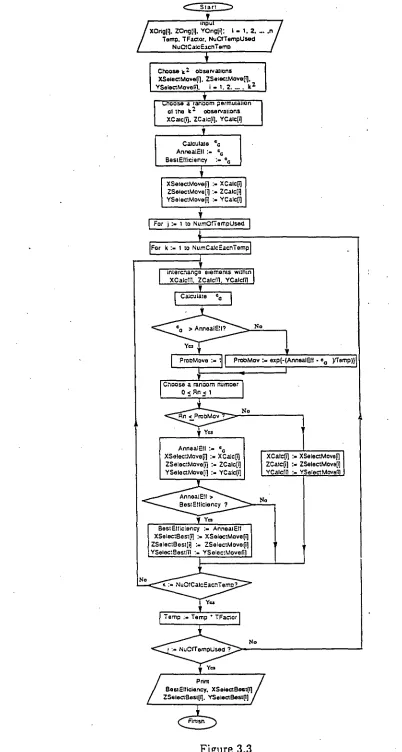
Simulated Annealing Method.

The arrays needed to store the data are as follows:

(i) (i) X0rig[i], ZOrig[i], YOrig[i], i = 1, 2, ... , n are used to store the original ordering of the data.

(ii) XSelectMove[i], ZSelectMove[i], YSelectMove[i], i = 1, 1, , k2 are first used to store the k2 observations selected, and then for storing an ordering of the k2 observations if it gives improved efficiency, or worse efficiency with probability as presented in (3.12).

(iii) XCalc[i], ZCalc[i), YCalc[i] are first used to store a random permutation of data and then to store an ordering of the data used for calculating e G .

(iv). XSelectBest[i], ZSelectBest[i], YSelectBest[i] are used to store the best ordering of the observations so far.

Some other variables used are : (i) Temp is used for temperature.

(ii) TFactor is the temperature multiplying factor.

(iii) NuOfTempUsed is the number of temperatures used in the process of getting the best efficiency. The temperature will decrease with the factor TFactor.

(iv) NuOfCalcEachTemp is the number of repeats of the procedure of calculating eG at each temperature.

(v) ProbMove is the probability of moving from one ordering of the data to others.

ProbMove <

f

=1 if eG AnnealEf f

[=

exp{—(Annea lEff — e G ) / Temp} if eG AnnealEff (vi) AnnealEff is used to record a new e_G each time we move to a new ordering of the data.

[image:37.558.82.484.20.772.2]

Figure 3.3

The flow—chart of the simulated annealing method

For 1 to NurnOfTerroUsed C_Sta

XOng[ii, ZOng[1]. YOrigtil; I . 1. 2. -. m Temp. TFactor. NuCITempUsed /

input

NuCtCatcEacnTemis

[For k 1 to NumCalcE.acnTemp

I

Temp Temp • TFactor I No

y YC71

/ BestElficie Prim ncy. XSelectElest(1] ZSetectElest(f). YSeiect8est(11

31

XSelectMove(i] XCalc(il ZSelectMove(11:. ZCalc(71 YSeiectMovegj YCalc(i)

Calculate eG AnnealEll eG

BestElficiency Choose k1 observations XSelectMove(fl. ZSeiectMove(T), YSelectMovera. i . 1. 2. k2

c.hoose a rancom permutation of the k2 ooservations XCalc(f). ZCatc(i). YCalc[il

I interchange elements within' I XCalefil. ZCalcfil. YCalc10 I

V

I

Calculate co

ProtiMove 1

_I

ProbMov exp(-(Annea8f yTernp)} > AnnealEff?

Yes

y Yea

AnnealEll eG

XSelec:Movecif XCalcgl ZSelectMove(i] ZCalc[i] YSelectMove(il YCalc[fl

XCalctil XSelectMovegl ZCalc[i] ZSelectMoveg] YCalefil YSeIectMovefll

Y02 BestElliciency AnneatElf XSelectEest(fl XSelectMovegj ZSelectBest(q ZSelectMoveill YselectEestfil YSelectMovell]

0

NuOtCaicEachTemo? 0

0

V

32

3.4. A Numerical Example.

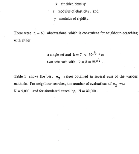
To illustrate how the method works, and to demonstrate that the necessary computer programming is relatively straightforward, the data from Maritz (1981) page 194 was used, where observations were modulus of rigidity of timber specimens, and design variables were

x air dried density

z modulus of elasticity, and y modulus of rigidity.

There were n = 50 observations, which is convenient for neighbour—searching with either

[image:38.562.44.509.236.750.2]

a single set and k = 7 < 501/2 ,or two sets each with k = 5 = 251/2 .

Table 1 shows the best e_G values obtained in several runs of the various methods. For neighbour searches, the number of evaluations of eG was

[image:39.559.77.486.169.465.2]

Table 3.1.

Efficiency of GLS to LS method

using Neighbour—searches and simulated annealing method.

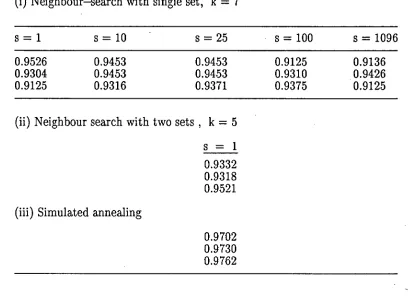
(i) Neighbour—search with single set, k = 7

S = 1 s = 10 s = 25 s = 100 s = 1096

0.9526 0.9453 0.9453 0.9125 0.9136

0.9304 0.9453 0.9453 0.9310 0.9426

0.9125 0.9316 0.9371 0.9375 0.9125

(ii) Neighbour search with two sets, k = 5

s = 1

0.9332 0.9318 0.9521 (iii) Simulated annealing

0.9702 0.9730 0.9762

For this example, the best performance is by the simulated annealing method.

We now continue to give a complete solution for this example. Suppose we choose the grouping which gave efficiency e G = 0.9762. The groups of observations are presented in matrix form as follows

34

x=

40.1 68.1 42.3 39.6 68.9 63.3 37.1 30.7 58.6 40.3 51.3 43.0 55.1 38.3 42.5 56.9 29.1 51.7 53.9 58.3 60.8 36.8 63.2 32.5 58.7 55.3 39.0 49.0 61.3 31.4 54.9 42.4 28.6 55.2 57.3 50.2 59.5 43.0 68.9 52.8 46.7 50.3 40.3 25.3 50.3 53.8 28.2 40.6 61.5

203 146 189 194 272 228 193 - 205 264 276 196 91 223 99

Z = 238 110 167 248 133 261 188 189 252 130 213 246 240

186 and 346 165 188 274 188 245 173

268 222 238 182 244 210 188 195 177 245 224 254 209 264

1587 1069 1492 1306 2054 1728 1145 1767 2036 1916 1746 925 1474 1000 1595 1438 1087 1306 1990 1605 1897 1254 1822 2129 2570 1129 2159 1676 2649 1647 1621 2086 1033 2053 1112 2604 1764 1870 1332 1909 1539 1281 1323 1379 2116 1706 1889 1703 1994

where the observations in the same row are in the same group. By using (3.5)

we obtain

AT = 10-3 (8.5919, -3.5517,.--4.8352, 6.4375, 6.8459, 2.8427, 4.2365)

35

z*T = (4.8885, 2.4273, 5.3664, 2.3963, 5.9581, 4.5989, 4.7556) and y*T = (34.8566 ,24.6856, 37.9711, 31.5204, 40.1202, 38.5121, 34.4414).

In the model

y. =

+ coc + fiz +c

i

with independent errors having zero expectations and common variance a 2 , from Appendix 1 we see that the full least squares estimate of is

3.319 with estimated standard error 0.81

After grouping and reducing the model to

y* = + fiz* + c* ,

1

the least squares estimate of /3 is

3.263 with standard error 0.85

36

e_G

=

0.9762. The discrepancy between the two efficiencies can be explained as follows. From Appendix 1 , we see that estimates of variance from ANOVA error mean squares are

var(e . ) = cr2 = 34,963.286,

and for the grouped case

var(c* ) = a*2 = 8.419.

7

Also we can calculate E A2 = 2.24152 x 10 The two efficiencies would be

7

the same if the assumption—estimate cr*2 = .72 E A2 was satisfied. Here we i.1

^ 7

have a2 E A2 = 7.8371 < (7*2 = 8.419, which explains why e > e.

Any exact method of inference for slope )3 in the simple linear regression model with y* regressed z* could now be used, and for this example we use the Brown and Maritz method (see Section 2.4). Since there are 7 observations, we have (7) = 21 values of )3. The point estimate and the

2 ij

confidence interval ,8 can be obtained more easily by using the graph of S( 13). The values of and their weights can be seen in Table 3.2.

Table 3.2.

The values of )3.. in ascending order and their weights.

Weight 37 -220.5673 -32.3527 -12.6198 -0.7049 0.8142 1.1831 1.3387 2.1719 2.4145 3.1743 3.6321 3.7605 4.1324 4.3714 4.5203 4.9124 5.5543 6.3669 6.5179 7.4166 10.6470 0.0310 0.1567 0.2897 0.7675 2.3593 1.3592 2.4923 2.9701 3.5618 2.2026 0.5917 2.3283 2.4613 3.5308 2.9371 1.0695 1.2025 2.1716 0.4778 0.6108 0.1329

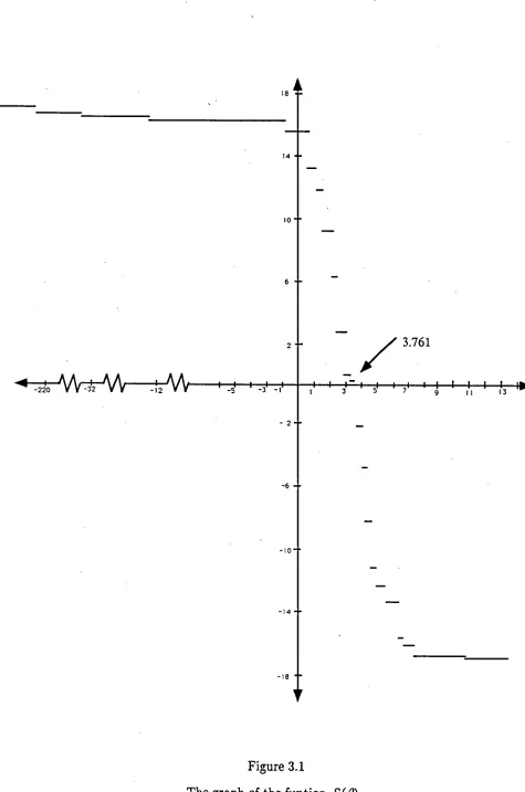
The formula (2.16) and (2.17) gives S(-o) = 16.8532 and

S(00) = -16.8532 and the graph is shown in Figure 3.1. The graph shows that

the solution for S = 0 is = 3.761 . From (2.15), we obtain

var(S) = 54.361 and therefore the standard deviation is 7.373. The 90

percent confidence interval of 3 can be calculated as follows

P(-1.645 < S < 1.645) = 0.90 7.373

Or

14 -

-

_

-

_

-

_

-

-

-

-

-

- -

-18 ""'

[image:44.561.57.532.49.766.2]

V

Figure 3.1

The graph of the funtion S(,(3) .

38

6 - 10

-14 -..-

3.319 (1.959, 4.680)

3.263 (1.550, 4.977)

3.761 (1.183, 4.921)

Full LS fl Grouped LL

Proposed )

39

and from the figure 3.1, we can obtain the 90 percent confidence interval of fi,

1.1831 < < 5.9214.

By the same method if the slope parameter a is of interest, with

eG = 0.9764 (the grouping matrices can be seen in Appendix 2), we obtain a point estimate of a = 16.764 and the 90 percent confidence interval of a is (13.367, 28.756).

The next table displays the estimate of slope parameters a and and their confidence interval by using the full least squares, grouped least squares and the proposed method.

Table 3.3.

The estimation of slope parameters a and 43 by using full least squares, grouped least squares and the proposed method

P

ara-meter Method Estimate Poi n t interval (90 %) Confidence

Full LS 20.305 (14.474, 26.136)

a Grouped LS 20.026 , ( 9.329, 30.722)

Proposed ) 16.764 (13.367, 28.756)

40

Table 3.3 shows that each 90 percent confidence interval of each slope parameter contains the three point estimates for that parameter. If the least squares assumptions hold, by using the

t test

with the same level of

CHAPTER 4

GENERAL LINEAR REGRESSION

In this chapter the method in Chapter 3 will be extended to situations where more than two independent design variables are taken into account. In order to avoid any confusion in notation when the observations are grouped, the general linear regression (1.1) is written again using superscript notation for the independent design variables as follows

Y. = 13 xl + x_{i 2i} 2 + + ,3 xP , i = 1, 2, ... , _{P1 i} n (4.1)

where n is the number parameters, x1, x2, , xP and identically distributed. interest and the other fl. (i

of observations, ,3 /3 are unknown o' 1, .. ' p

are design constants, { ei} are independent errors Without loss of generality suppose that 131 is of #1) are the nuisance parameters. The next step is to eliminate the nuisance parameters such that the general linear equation (4.1) can be reduced to a simple linear form.

2.1. Method of Parameter Elimination.

To eliminate the nuisance parameters fi. (i 0 or 1) and reduce the model to SLR form, the observations are placed into

k = Rn/(p-1)11/21 (4.2)

groups, where n is the number of observations and p is the number of

42

independent design variables. Thus the number of observations allocated in each group is m = (p-1)k.

Let A , A , .

• . , A be constants, and for i = 1, 2, ... , k define 12 m

m m m m

y*.= A.y. i ,

Jr 1

= 0 A+/3 1 Ax , N

irl

+,6 Ax

j1

2 f \

1 1 j+Mki-1) 0 . j 1 j., j j+ mki-1) 2 j j+mki-1)

=

m m

Ax Pj+m(i-1) + 1 A:E (4.3) j=1 J • J

Suppose that {Ai } are chosen so that for all r = 2, 3, ... , p

m m m

A .xr. = 1 A.xr. = A xr =... .1 ,4 J J j=i J .14-111 iri j j+2M

= constant, x* say.

r

Then from (4.1) , (4.3) and (4.4)

y* = ,3*+ 13z* + c* i i

where y* =E A y I \ )51* = c + )(3 _j x* , c= A

j j+mki-i) o o j=2 j j=1 j , Z* = E A x1

jr1 i+mki-1) j \ and e* = j=i A e j+mo j f -1) . The equation (4.5) is of SLR form because {e*.} are independent and identically distributed, and so can be treated by exact DF methods.

How can {A . } and fx*1 be chosen so that (4.4) holds? Let k x m matrices X ,X , ,X be such that

2 3 p

(4.4)

X =(X) =x2 f

2 2

X = (X ) =x3 \

3 3 i)j

X = ) = XP

p j

If AT = (A , A , . , A )uT = (x*, x*... x* ••• x* x* ... x*) and X is

12 m ' — 2 2 2 p p p

an m x m matrix such that

- X - 2

X

43

3

x

=

then we need to find A and u satisfying (4.4) , i.e.

X A = u ,

and if X- is a non—singular matrix we get

A = X-1 u . (4.6)

44

After defining a suitable A , the k pairs of values {z*., y*} for the SLR

model (4.5) can be obtained more easily by using matrix notation. Let k x m matrices Z and Y be such that (Z) = x 1 and _i+m(i-1) (Y)

1 = y j+mk ,i f i-i) If Z*T = (Z *1 2 k 7 Z*7 ... 7 z*) and y* T = (y*, y*, ,y*) then 1 2

z* =

Z A

y* = Y A (4.7)

We have reduced the general linear model (4.1) with n observations to the simple linear regression model (4.5) with k observations.

4.2 Minimizing the Loss of Efficiency.

After reducing the model, the further steps are similar to the steps which we discussed in Chapter 3. Our aim is to maximize the grouping efficiency eG , and to that end the approximation methods for finding the

best grouping as described in Section 3.3 can be used.

If equation (4.1) is written in a matrix notation, we have y = A 9 + , where

1 x1 x2 ...x _{1 1 1} xP

1

X1 X2 ... XP 2 2 2 A

45

= (y1, Y27 Yn) 7 0T /61,

flp

) and = ( 11, 121 7

(0) LS is the ungrouped least squares estimate of /3 then from (2.7)

var{(fl)Ls} = 02{ATA)--1122

where

e

is the observational error variance. To get var

{(13 where (1)GLS 13 is the least squares estimate of after grouping, we write [3

1)GLS }

y* = A*

0

+

c

where y*T = (y)C y* ,

21 k

1 Z*

1

1 Z*

2

A* =

0*T = (15)* ) and c*T = f*, , c*k) , and by (2.7) o'

Var{(131)GLS} = e2{(A*TA1-11₂₂

where o-*2 = var(e) = E A2 . Thus the relative efficiency of grouped to j=1 j

46

(ATA ) 22

A2 (A*TA*)-41

i 22

To maximize e_{G '}

var{ (131)GLs} must be minimized, that is groups

are to be chosen to minimize

A2

=

{A*T.A*}-11 A2 = m

j1

• (4.9) 22

z*2 z*)2/k j =1

The values of (4.9) depend on the choice of A and u corresponding to allocation of the observations into the k groups.

The vector uT = (x*2, x*2, , x*2, , x*, x*, x*) can be written

P P

as

U = V u* (4.10)

where u* = (x*

' x*' , x*) and V is an m x (p-1) matrix such that if

2 3 p

and 0T

=

(0, 0, , 0) then

-k -k

1 0 ...O

—1 —1 —k

0 1 ... 0

—t —1 —k

0 0 ... 1

-t -t -t

Now (4.6) can be written as

A = X-1 V u* = M u* (4.11)

where M = X-1 V . By (4.7) and (4.11) each term of the the denominator of (4.9) can be writen as

V „*2 = „*T ,* _*T _{MT z}T 7 As ..*

41 11

j=1 and

z* )2/k = (z*T 11T _* *T T

k— — Z = kU M Z 1T Z M u*)/k

j=1

where 1T = (1, 1, , 1). Now we can write (4.9) as

in

{(A*TA*)-1} A2 =

22 j irl

T

u* MT M u

(4.12)

u*T MT ZT _{P Z M u*}

47

-

=

48

u*T C u*

P =

u*T B u* (4.13)

where C = MT M , B = MT ZT P Z M. By differentiating p with respect to the elements of u* , and equating to zero, we obtain

(u*T B u*) C u* = (u*T C u*) B u*

that is

(C — p B) u* = 0 . (4.14)

In general C and B are non—singular, so there are two possibilities for solving (4.14); that is

(i) B (B-1C — pI) u* = 0 (4.15)

where u* is an eigenvector of B -1 C corresponding to the eigenvalue p ,

and since our aim is to minimize p, p must be the minimum eigenvalue of C ;

and

49

where u* is an eigenvector of C-1 B corresponding to the eigenvalue p-1 , so to minimize p, p-1 must be the maximum eigenvalue of C-1 B.

So to choose e_G optimally , (i) find the minimum eigenvalue p of

B-1 C = NIT p z mr1 mT m

-1 or the maximum eigenvalue p of

C-1

B =

_(MT m) -1 MT zT p z m

(ii) set u* = the corresponding eigenvector, and the resulting maximal value of e_{G '} from (4.12) , (4.9) and (4.8) , is

e = {(AT . (4.17)

22

Now we can maximize the grouping efficiency eG by using one of the three methods of finding approximate solutions as oulined in Section 3.3.

4.3. A Numerical Example.

This example is taken from Feldman et al (1986) page 31 (demonstration data) where the observations are the cholesterol (y), cholesterol at 1 years old (xl.), weight (x2.) and the tryglicerides (x3.). With model y. = /3 + xi + fix2 + c , suppose /3 is of interest. Here m = 2,

o 2i i

(&3

50

so the 50 observations are divided into k = [50/211/2 = 5 groups, each containing 10 observations. Because # is of interest, let Y, Z, X2, and X

3

be 5 x 10 matrices such that

Y = (y)j+5(1-1)

(xIdi+s(i-1) X = (X ) = (x2) f

2 2 bj i j+50-1)

X = (X ) = (X3) I \

3 3 I j+50-1)

and then form the 10 x 10 matrix

X

X = [-)-! 1. (

3

After using the simulated annealing method, we obtained an approximation of the best grouping which gave efficiency eG = 0.9374 with

(i) p-1 = 32832.50622848 ,

97614.6279807 —116468.3150964 I

(ii) C-11 B = , and

(iii) the grouping matrices as follows

139 149 134 168 162 110 152 172 170 177 - 183 156 116 191 170 138 146 154 201 122 123 178 155 168 165 175 154 167 187 173 125 205 160 158 165 162 177 153 201 166 163 150 192 208 187 115 150 121 136 154 148 61 53 98 79 65 60 100 105 135 92 81 118 57 88 71 68 64 85 79 59 85 69 96 91 118 69 105 95 82 85 53 103 57 116 98 32 96 79 70 59 167 47 65 85 184 73 105 145 89 _

173 142 135 178 203 176 185 134 191 229 179 171 180 167 185 176 172 148 175 185 187 209 223 210 137 186 149 273 182 160 165 139 159 145 228 189 179 136 177 200 190 249 172 182 162 224 167 244 200 175

172 142 133 158 192 169 178 134 184 219 - 172 151 170 167 180 171 161 148 162 180 177 189 201 190 137 166 145 253 182 168 164 129 152 135 208 182 159 130 188 221 188 222 167 172 155 219 167 224 191 145 _

Note that all of the notations and definitions are the same as in Section 4.2.

Thus an eigenvector of C-1 B corresponding to

p

-1

is

u*

T

=

(1, 0.5562210).

By using (4.11) we obtain

AT = 10-3(1.541370, 2.562477, 3.256696, 1.348090, —2.749399, —1.049215, —1.332395, 5.295262, —0.5206508, —1.795876)

51

X

z=

and then by (4.7)

*T

z =

(0.519725, 0.963300, 2.126295, 0.528960 ,1.707120) *T

= (0.553226, 0.918092, 1.867065, 0.479284, 1.582235)

In the model y = + /3 + x2 + x3 + e with independent errors i 0 li 2i 3i i

having zero expectation and common variance cr2 , from Appendix 3 the full least squares estimate of a is

0.853 with estimated standard error 0.047 .

After grouping and reducing the model to y* = 13* + z* + e* , the least

0 1

squares estimate of becomes

0.858 with estimated standard error 0.033 .

As in the numerical example of Section 3.4 , the discrepancy between the full least squares and the grouped least squares point estimate of /3 is 0.005 with pooled standard error > 0.033 , and is almost certainly due to sampling variation. The discrepancy between e G = 0.9365 , and an empirical relative efficiency calculated from the two standard errors above, that is e = 2.0285 ,

5

is related to the fact that the assumption—estimate a*2 = a2 E A' was not J1

satisfied . From Appendix 3 we see that estimates of variance from ANOVA error mean squares are

52

var(c . ) = 78.113 ,

and for the grouped case

var(c*) = 0.002 .

5

Also we can calculate E A2 = 6.333690 x 10-5 , so

^ 5

u

2

E A

2

=

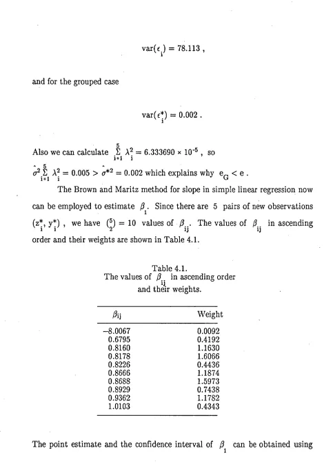
0.005> 0**2 = 0.002 which explains why e G < e .

The Brown and Maritz method for slope in simple linear regression now can be employed to estimate Since there are 5 pairs of new observations (z, , we have (5) = 10 values of. The values of /3 • in ascending

2 ij ij

[image:59.562.51.521.47.724.2]

order and their weights are shown in Table 4.1.

Table 4.1.

The values of fi.. in ascending order and their weights.

Weight

—8.0067 0.0092

0.6795 0.4192

0.8160 1.1630

0.8178 1.6066

0.8226 0.4436

0.8666 1.1874

0.8688 1.5973

0.8929 0.7438

0.9362 1.1782

1.0103 0.4343

53

4

3

2

54

0.8666

-8 .1 .6 .8 .9 .0 1

-2

-3

-4

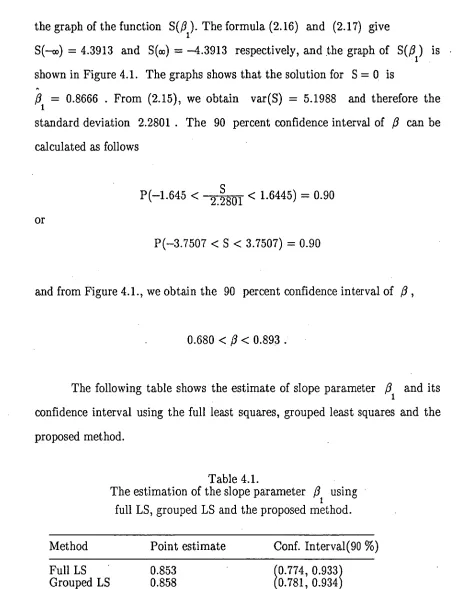
[image:60.562.51.527.43.750.2]

Figure 4.1

55

the graph of the function S(3). The formula (2.16) and (2.17) give

S(—co) = 4.3913 and S(co) = --4.3913 respectively, and the graph of S((3 1) is shown in Figure 4.1. The graphs shows that the solution for S = 0 is

= 0.8666 . From (2.15), we obtain var(S) = 5.1988 and therefore the standard deviation 2.2801 . The 90 percent confidence interval of )3 can be calculated as follows

P(-1.645 < 2101 < 1.6445) = 0.90

Or

P(-3.7507 <S < 3.7507) = 0.90

and from Figure 4.1., we obtain the 90 percent confidence interval of /3,

0.680 <3 < 0.893.

[image:61.559.61.523.94.683.2]

The following table shows the estimate of slope parameter /31 and its confidence interval using the full least squares, grouped least squares and the proposed method.

Table 4.1.

The estimation of the slope parameter fit using full LS, grouped LS and the proposed method. Method Point estimate Conf. Interval(90 %) Full LS 0.853

Grouped LS 0.858 0.774, 0.931 0.781, 0.934

56

CHAPTER 5

DISCUSSION AND CONCLUSION

5.1. Discussion.

In this section we discuss another possible way of grouping the observations in planar regression (see Section 3.1), a possible way to sidestep the difficulties of obtaining the eigenvector p for example when both of the matrices MT ZT P Z A and MT M are "nearly" singular (see Section 4.2), and a possible method to speed up the the simulated annealing convergence for a relatively large sample size.

As an effect of grouping of observations, usually all of the observations cannot be used to estimate the parameter of interest, and therefore the observations used to estimate the parameter of interest must be chosen randomly from the observations available. The numerical example of Section 3

4,

shows that just 49 of 50 data available were used. If the number of data used is less than the number of observations available, then there is a loss of information needed to estimate the slope parameter of interest. For planar regression, to maximize the number of observations used (and also the efficiency of grouping), we can combine a variation of neighbours search method (i.e. divide data into two or more separate sets and carry out the grouping operations separately within each set, see Section 3.3.2.) and the simulated annealing method. The variation ofVfieighbours search method is used to maximize the number of data used and the simulated annealing method to maximize groupings efficiency. If observations are divided into m sets, k is the number of groups in each set, and n is the number of observations, then

58

k = mn 1:12

The combined method helps us to maximize the number of data used, but implies extra work to estimate the parameter of interest. Because the m sets of observations give m independent estimates of the parameter of interest, then the parameter of interest can be estimated using a linear combination of the m estimators. In the numerical example of Section 3.5 , if we choose m = 2 , all of the 50 observations can be used to estimate # .

In Section 4.2 , we maximize the grouping efficiency eG by minimizing

var{ _(13i) I

•GLS'' and in so doing need an approximation to the minimum

eigenvalue p of (MT zT p z •) - A 1 MT M or the maximum eigenvalue p' of

(MT -T _{m ZT P Z A . After obtaining}

p or p-1 we calculate u* as the

corresponding eigenvector, but can encounter problems for example in case both of the matrices MT ZT P Z A and MT M are nearly singular. To sidestep such problems we choose u* = 1. With this choice from (4.6) we obtain

Using the choice of u* = 1 to solve the numerical example of

Section 4.3 , gave an approximation of the best efficiency eG = 0.9365 (the

59

The proposed method involves solving a difficult combinatorial optimization problem with the simulated annealing method showing the best performance. The method is quite computer intensive and to give good results, lengthly computer runs may be necessary. Because the method of grouping used implies n! possible groupings (many will share the same value of e G ), the computing time needed to get an approximate solution will depend on sample size, the number of independent design variables and which approximation method is used.

For a relatively large sample size, to speed up the the simulated annealing convergence, instead of interchanging one or more pairs as described in Section 3.3.3 , we choose r observations at random ( r also is chosen

randomly, 2 < r < k2), and then permute the order of the r observations selected randomly. Preliminary experience shows that if r is restricted so that it is not too large (say 2 < r <

10 ),

then there is a considerable reduction in computing time.

5.2. Conclusion.

In this thesis we have proposed an exact distribution—free method of solving general linear regression problems, where one of the slope parameters is of interest, through grouping of observations to eliminate the nuisance parameters and reducing the model to simple linear regression form, and then using an exact distribution—free method for slope in simple linear regression.

60

involves all of the general linear regression problems with error terms satisfying the above assumptions.

The method is a simpler alternative to the Maritz—Theil approach, and also gives satisfactory efficiency, especially for the planar regression. The efficiency will decrease if the number of independent design variables increases. There are two factors causing a loss of efficiency, that is grouping and reducing the model (eliminating the nuisance parameters). Grouping eliminates the individual character of data in that it ignores the variation of data within each group and then replaces them with a new value, and reducing the model eliminates the individual effect of each nuisance parameter. The above information explains why the grouping efficiency will decrease if the number of independent design variable increases.

Confidence Intervals and Partial F Table

95n Lower: 95% Upper: 90% Lower: 90% Upper: Partial F:

Variable:

R-sauared: Ad i. R-sauared: RMS Residual: Count:

149

1.9

1.8 1 1.802 1186.985

Analysis of Variance Table

Sum Sauares: Mean Square:

DF: F-test:

Source

Beta Coefficient Table

Std. Err.: Std. Coeff.: t- Value: Probability:

Variable: Coefficient:

Multiple Regression Y :var y 2 X variables

REGRESSION 2 6857621.081 3428810.54 98.069

RESIDUAL 46 1608311.164 34963.286 p =0001

TOTAL 48 8465932.245

No Residual Statistics Computed

Multiple Regression Y :vary 2 X variables

INTERCEPT -13.607

var x 20.305 3.473 .565 5.846 .0001

var z 3.319 .81 .396 4.096 .0002

Multiple Regression Y 1 :var y 2 X variables

INTERCEPT

var x 13.312 27.297 14474 26.136 34.175

var z 1.688 4.951 1.959 4.68 16.776

61

Appendix 1

The least squares solution of the numerical example of Section 3.4.

Simple Regression X 1 : variable z Y : variable y

: R-sauared: Ad i. R-sauared: RMS Residual:

Count:

1.696 12.902

7 1.864 1.747

Analysis of Variance Table

Sum Sauares: Mean Sauare:

DF: F-test:

Source

Coefficient: Std. Err.: Std. Coeff.: t-Value: Probability: Variable:

INTERCEPT 20.275

3.839 .0121

.85 .864

SLOPE 3.263

Confidence Intervals Table

95% Lower: 95% Upper: 90% Lower: 902 Upper:

Variable.

REGRESSION 1 124.061 124.061 14.735

RESIDUAL 5 42.097 8.419 0 =.0121

TOTAL 6 166.159

No Residual Statistics Computed

Simple Regression X i : variable z Y : variable y

Beta Coefficient Table

MEAN (X,Y) 31.624 37.264 32.234 36.654

SLOPE 1.078 5.449 1.55 4.977

2. The grouped least squares.

Appendix 2

The grouping matrices for slope parameter a for the numerical example of Section 3.1'

x=

146 223 213 222 346 209 245 264 210 165 248 264 182 110 276 244 224 254 268 274 238

130 205 196 186 188 188 194 133 252 167 272 91 99 188 195 261 245 246 189 188 228 193 189 240 177 173 238 203

30.7 59.5 43.0 42.4 68.1 63.2 53.8 55.1 68.9 50.3 40.6 28.6 36.8 29.1 52.8 58.6 46.7 54.9 40.3 61.3 31.4 43.0 51.3 61.5 25.3 32.5 37.1 51.7 39.0 39.6 56.9 60.8 68.9 58.7 53.9 55.2 49.0 57.3 50.2 40.3 42.5 50.3 63.3 55.3 58.3 38.3 28.2 42.3 40.1 _

1069 1474 1605 1129 1767 1746 1676 1764 2649 1703 1281 1033 1306 1087 2053 2036 1539 1990 1438 2054 925 1647 1822 1994 1000 1306 1323 2129 1332 1254 1916 2116 2159 2570 1621 1909 1706 1889 1728 1145 1492 1897 2604 2086 1870 1379 1112 1595 1587

63

Confidence Intervals and Partial F Table

95g. Lower. 95% limier: 90% Lower: 90% Upper: Partial F:

Variable:

Analysis of Variance Table

Sum Sauares: Mean Sauare:

DF: F-test:

Source

Beta Coefficient Table

Std. Err.: Std. Coeff.: t- Value: Probability:

Variable: Coefficient:

Multiple Regression Y _i :Cholestrol 3 X variables R-sauared:

1.903

Ad 1. R-sauared: RMS Residual:

1.897 18.838

R : Count:

REGRESSION 3 33478.596 11159.532 142.865

RESIDUAL 46 3593.184 78.113 p =0001

TOTAL 49 _ 37071.78

No Residual Statistics Computed

150

1.

95

Multiple Regression Y _i :Cholestrol 3 X variables

INTERCEPT 17.65

Chol-lvr .853 .047 .948 18.068 .0001

Weiaht .002 .054 .002 .036 .9716

Trialvcerides .005 .049 .006 .103 .9186

Multiple Regression Y I :Chol estrol 3 X variables

INTERCEPT

Chol-Ivr .758 .948 .774 .933 326.45 I

Weiaht -.106 .11 -.088 .092 .001

Trialvcerides -.093 .103 -.077 .087 .011

64

Appendix 3

The least squares solution of the numerical example of Section 4.3.

Ad i. R-sauared: RMS Residual:

: R-sauared:

Count:

1.994 1.047 1.998 1.996

5

Analysis of Variance Table

Sum Sauares: Mean Sauare:

DF: F- test:

Source

Variable: Coefficient: Std. Err.: Std. Coef f.: t-Value: Probability:

952 Lower: 95% Upper: 90% Lower: 90% Upper:

Variable:

Simple Regression X 1 : variable z* Y : variable y*

REGRESSION 1 1.53 1.53 694.48

RESIDUAL 3 .007 .002 p = .0001

TOTAL 4 1.536

No Residual Statistics Computed

Simple Regression X 1 : variable z* Y : variable y*

Beta Coefficient Table

INTERCEPT .077

.0001 26.353

.998 .033

.858 SLOPE

Confidence Intervals Table

MEAN (X ,Y) 11.013 1.147 1.031 1.129

SLOPE .754 .961 .781 .934

2. The grouped least squares