Macaulay's method for a Timoshenko beam

Macaulay’s method for a Timoshenko beam

N. G. Stephen

School of Engineering Sciences, Mechanical Engineering, University of Southampton, Highfi eld, Southampton SO17 1BJ, UK

E-mail: [email protected]

Abstract The Macaulay bracket notation is familiar to many engineers for the defl ection analysis of a Euler–Bernoulli beam subject to multiple or discontinuous loads. An expression for the internal bending moment, and hence curvature, is valid at all locations along the beam, and the defl ection curve can be calculated by integrating twice with respect to the axial coordinate. The notation obviates the need for matching of multiple constants of integration for the various sections of the beam. Here, the method is extended to a Timoshenko beam, which includes the additional defl ection due to shear. This requires an additional expression for the shearing force, also valid at all locations along the beam.

Keywords Macaulay; bracket notation; Timoshenko beam

Notation

A cross-sectional area

C constant of integration

E Young’s modulus

G shear modulus

I second moment of area

L length of beam

M moment

P applied force

Q shearing force

R reaction force

u, v displacement components in x and y directions

w uniformly distributed load

x, y planar Cartesian coordinates

k shear coeffi cient

y cross-sectional rotation

Introduction

Macaulay’s method is a familiar topic within many ‘mechanics of solids’ modules forming part of mechanical, aerospace and civil engineering undergraduate degree programmes [1]. The method is, in essence, a fi rst exposure to (and pre-dates) gen-eralised functions (e.g. Dirac delta, step, and ramp), with meaning given over to the bracket notation, typically of the form [x− a]n

bending moment within a beam structure produced by uniformly distributed loading (UDL) when one has n= 2, concentrated (or point) force loads when n= 1, and point moments when n= 0. Moreover, the load is located (or commences in the case of a UDL) at x=a, leading to an obvious mathematical structure. Having so derived an expression for the bending moment which, using this notation, is valid at any location along the beam, the moment–curvature relationship for the (small-slope) Euler–Bernoulli model is:

M EI v

x = ± d

d

2

2

where the positive or negative sign depends upon the sign convention employed. This allows calculation of the transverse defl ection, v(x), by integrating relatively simple functions twice with respect to the axial coordinate, x. In practice, the inte-gration is performed with respect to the argument of the bracket, rather than x, in order to keep the bracket and its meaning intact. For example, x integrates as

x2

/2 in the normal way, but [x − a] integrates as [x − a]2

/2. Treated normally, x−a x x ax C

( ) = − +

∫

d 2

1

2

/ , where C1 is a constant, whereas if integrated with

respect to the argument,

∫

[x−a] = −dx [x a]2/2+C2, where C2 is also a constant.

The difference lies in the value of the two constants of integration, the latter expression having the additional constant term a2

/2; this difference is resolved so long as the constants are evaluated with the meaning of the brackets taken into account.

Macaulay’s method is ideal for the calculation of the defl ection of beam structures subject to a variety of loads along their span, including statically indeterminate systems. While the method is widely attributed to Macaulay [2], his being the fi rst English-language description, Weissenburger [3] has provided some historical perspectives that indicate that the approach goes back to Clebsch in 1862. It has been generalised by Wittrick [4], who considered Euler–Bernoulli beams includ-ing axial compression and elastic foundations, as well as circular plates with a variety of discontinuous loads. Recent papers by Yavari et al. [5–8] have provided a variety of research results, including application to Timoshenko beams, elastic foundations and to cases in which the bending and shear stiffness properties change abruptly.

is suffi cient to note that the governing equations for the Timoshenko beam model are:

M EI x = d

d

ψ

and

Q AG v

x =κ

( )

d +ψ

d

where we employ the sign conventions from Reismann and Pawlik [9]. This implies that one requires expressions for both the bending moment and the shearing force that are valid at all locations along the beam.

Finally, note that Wang [10] has presented relationships between the slope, defl ec-tion and support reacec-tions of a single-span Timoshenko beam, for a variety of end conditions, in terms of their Euler–Bernoulli counterparts. The present work shows that the Timoshenko beam can be treated from fi rst principles in much the same way as a Euler–Bernoulli beam, with little added complexity.

Example 1

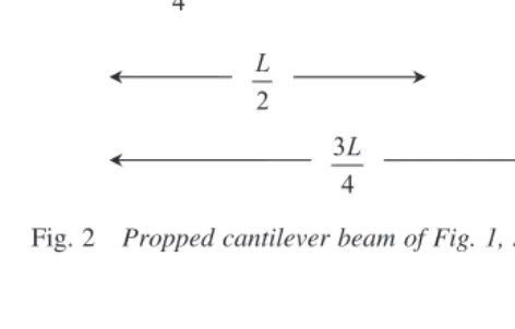
The fi rst example is shown in Fig. 1 and consists of a propped cantilever beam subject to two point loads, a point moment and partial UDL. In Fig. 2, the complete structure is shown with the support reactions. Vertical force equilibrium requires:

RA+RB= + +P1 P2 wL

4 (1)

3 4

L y,v

x,u L

4 L

1 P

2 P

2 L

1

M w

[image:3.514.38.325.349.553.2]

B A

Moment equilibrium (about the left-hand end) requires: MA+RB L =M +P L+P L+w

( )( )

L L

3

4 4 4

5 8

1 1 2 (2)

At this stage one has three unknown reactions, but just two equations; the third is derived from the expression for the defl ection curve.

Cut the beam at some generic cross-section x close to the right-hand end, and insert a shearing force, Q, and a bending moment, M, as shown in Fig. 3. As is conventional, the UDL is continued on the upper surface, but negated by the intro-duction of an equal but opposite UDL on the lower surface. This has no effect on either the shearing force or the bending moment, but is necessary because the bracket notation ‘switches on’ the load, and an alternative device is required to switch it off. Vertical force equilibrium requires:

3 4

L L

4 L

1 P

2 P

2 L

1

M w

B

R

A

R

A

[image:4.514.64.314.218.361.2]

M

Fig. 2 Propped cantilever beam of Fig. 1, showing support reactions.

3 4

L 4

L

1 P

2 L

1

M w

B

R

A

R

A

M _M

Q x

w

[image:4.514.65.302.401.552.2]

Q+RA+RBx− L w x L P x L w x L   +  − =  −  +  − 

3 4

3

4 4 2

0

1

0

(3) Moment equilibrium about the cut face requires:

M M x L R x R x L w x L

P x L

A B +  −   + +  − +  −  =  −  1 0 2 1 2 3 4 2 3 4 4  +  −  + w

x L MA

2 2 2 (4) Now, set M EI x = d d ψ

and integrate to give:

EI M x L R x R x L w x L

P x

A B

ψ +  −

 + +  −  +  −  = 1

2 2 2

1

2 2 2 3 4 6 3 4 2 −−    +  −  + + L w

x L M xA C

4 6 2

2 3

1

(5)

Apply the boundary condition y(0) = 0 to give C1= 0.

Now rearrange the expression

Q AG v

x

v x

Q AG

=κ

( )

ψ+ = −

κ ψ

d d as

d d

and substitute from equations 3 and 5 to give:

d d

v

x AG P x

L

w x L RA RB x L w x L

=  −   +  − − −  −  − − 1 4 2 3 4 3 1 0 0

κ 44

1

2 4 6 2 2

1 2 3 1          −  −   +  −  + −  − EI P

x L w x L M xA M x L

 −    −  −   −  −  _ R x R

x L w x L

A B 2 2 3 2 2 3 4 6 3 4 (6)

Integrate to give: v x

AG P x

L w

x L R xA RB x L w x

( )=  −

 +  −  − −  − − −

1

4 2 2

3 4 2 1 2 κ 3 3 4 1

6 4 24 2 2

2

1

3 4 2

L

EI P

x L w x L M xA M

         −  −   +  −  + − 1 1 2 3 3 4

2 2 6

6 3

4 24 3

4

x L R x

R

x L w x L

A B −    −    −  −   −  −    ++C2

Apply the boundary condition v(0) = 0 to give C2= 0. The third equation necessary

to determine the reactions derives from the further boundary condition v 3L

4 0

( )

= , to give:

0 1

2 2 4

3 4

1

6 2 24 4

1

2

1

3 4

= _

( )

+

( )

−

( )



 

−

( )

+

( )

+ κAG P

L w L

R L

EI

P L w L M

A

A

2 2

3 4

2 4 6 3

4

2

1

2 3

L

M L RA L

( )

  

−

( )

−

( )

 

(8)

While equation 8 can be simplifi ed by the introduction of a dimensionless stiffness parameter of the form (EI/kAGL2

), these equations are of considerable complexity and little is gained by proceeding to full expressions for the reactions, and the analysis is not pursued further.

Example 2

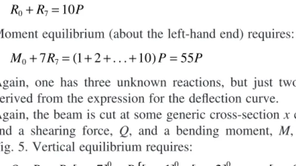
The second example is also a propped cantilever beam, now subject to multiple point loading, as shown, with support reactions, in Fig. 4. Vertical force equilibrium requires:

R0+R7=10P (9)

Moment equilibrium (about the left-hand end) requires:

M0+7R7= + +(1 2 . . .+10)P=55P (10) Again, one has three unknown reactions, but just two equations, with the third derived from the expression for the defl ection curve.

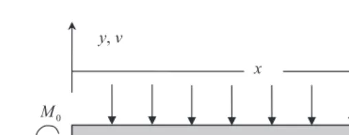
[image:6.514.31.356.85.147.2]

Again, the beam is cut at some generic cross-section x close to the right-hand end, and a shearing force, Q, and a bending moment, M, are inserted, as shown in Fig. 5. Vertical equilibrium requires:

Q+R0+R x7[ − ] =P

{

[x− ] + −[x ] + + −[x ]

}

0 0 0 0

7 1 2 . . . 9 (11)

y,v

x,u 10

7 R 0

R 0 M

[image:6.514.35.337.381.550.2]

Moment equilibrium requires

M+R x0 +R x7[ −7] =M0+P{[x−1]+ −[x 2]+. . .+ −[x 9]} (12) Again, set

M EI x = d

d

ψ

in equation 12 and integrate to give:

EIψ +R x0 + R [x− ] =M x+ P

{

[x− ] + −[x ] + + −[x ]

}

+C 2

7 2

0

2 2 2

1

2 2 7 2 1 2 . . . 9 (13)

Again, the constant C1= 0, on account of the boundary condition at the left-hand

end, y(0) = 0. Now, construct

d d

v x

Q AG

= −

κ ψ

and integrate to give:

v x P

AG x x x

R x AG

R AG x M x

EI

( )= {[ − ]+ −[ ]+ + −[ ]}− − [ − ]

−

κ 1 2 9 κ κ 7

2

0 7

0 2

. . .

++R x + [ − ] −

{

[ − ] + −[ ] + + −[ ]

}

+ EI

R EI x

P

EI x x x C

0 3

7 3 3 3 3

2

6 6 7 6 1 2 . . . 9

(14)

And again, the constant C2= 0, on account of the boundary condition at the left-hand

end, v(0) = 0.

The necessary third equation derives from the further boundary condition,

v(7) = 0, to give:

0 6 5 1 7 7

2 7

6 6 6 5 1

0 2

0 3

0 3 3 3

= P { + + + }− − + −

{

+ + +

AG

R AG

M EI

R EI

P EI

κ . . . κ . . .

}}

(15)

The reactions are then calculated as: y,v

x

7 R 0

R 0

M M

[image:7.514.61.315.43.141.2]

Q

R7 P ₂ R0 P M0 P

7 1

52 7

3 1

6 7

3 1 1 2

= +

( γ)

( )

+γ , = +γ

( )

+γ , = +γ ( + γ) (16) where γ

κ = 3

72 EI

AG

Note that the reactions for the Euler–Bernoulli beam are found by setting g= 0. It is now straightforward to substitute into equations 11, 12 or 14 to give expressions for the shearing force, bending moment and transverse defl ection that are valid at all locations along the beam.

Conclusions

By way of two worked examples, Macaulay’s method has been extended to the defl ection analysis of the Timoshenko beam model. One now requires general expressions for both the bending moment, as in the treatment of a Euler–Bernoulli beam, and the shearing force that are valid at all locations along the beam.

References

[1] P. P. Benham, R. J. Crawford and C. G. Armstrong, Mechanics of Engineering Materials (2nd edition) (Longman, Harlow, 1996).

[2] W. H. Macaulay, ‘A note on the defl ection of beams’, Messenger of Mathematics, 48 (1919), 129. [3] J. T. Weissenburger, ‘Integration of discontinuous expressions arising in beam theory’, AIAA

Journal, 2(1) (1964), 106–108.

[4] W. H. Wittrick, ‘A generalization of Macaulay’s method with applications in structural mechanics’,

AIAA Journal, 3(2) (1965), 326–330.

[5] A. Yavari, S. Sarkani and E. T. Moyer Jr, ‘On applications of generalized functions to beam bending problems’, International Journal of Solids and Structures, 37(40) (2000), 5675–5705.

[6] A. Yavari, S. Sarkani and J. N. Reddy, ‘Generalised solutions of beams with jump discontinuities on elastic foundations’, Archive of Applied Mechanics, 71(9) (2001), 625–639.

[7] A. Yavari, S. Sarkani and J. N. Reddy, ‘On nonuniform Euler–Bernoulli and Timoshenko beams with jump discontinuities: application of distribution theory’, International Journal of Solids and Structures, 38(46–7) (2001), 8389–8406.

[8] A. Yavari and S. Sarkani, ‘On applications of generalized functions to the analysis of Euler– Bernoulli beam-columns with jump discontinuities’, International Journal of Mechanical Sciences,

43(6) (2001), 1543–1562.

[9] H. Reismann and P. S. Pawlik, Elasticity, Theory and Applications (Wiley, Chichester, 1980), pp. 221–222.