Teaching calculus using dynamic geometric tools

(1)

This book was completed in the context of the CALGEO project (Calculus & Geometry). This project was co-funded by the European Commission under the framework of the European program SOCRATES, action COMENIUS 2.1. In the book are educational activities which were developed through the CalGeo project concerning the teaching of Mathematical Calculus/Analysis using the Dynamic Geometry software EucliDraw.

The CalGeo project involved the National & Kapodistrian University of Athens (coordinating institution), the University of Crete, the University of Southampton, the University of Sofia and the University of Cyprus.

Edited by:

Theodossios Zachariades, Keith Jones, Efstathios Giannakoulias, Irene Biza, Dionisios Diacoumopoulos & Alkeos Souyoul

Contributors: T. Zachariades, P. Pamfilos, K. Jones, R. Maleev, C. Christou, E. Giannakoulias, R. Levy, L. Nikolova, G. Kyriazis, D. Pitta-Pantazi, I. Biza, D. Diacoumopoulos, A. Souyoul, N. Bujukliev, N. Mousoulides, & M. Pittalis

CALGEO project was co-funded by the European Commission, SOCRATES - Comenius Action 2.1

Training of School Educational Staff

(Project Number: 118982-CP-2004-GR-COMENIUS-CS1) http://www.math.uoa.gr/calgeo

CALGEO

CALG

EO Te ac hi ng Ca lc ul us us in g D yn am ic G eo m et ri c To ol s

Teaching Calculus using

Dynamic Geometric Tools

National & Kapodistrian University of Athens, Greece University of Crete, Greece

(2)

Teaching Calculus

Using

Dynamic Geometric Tools

National & Kapodistrian University of Athens, Greece University of Crete, Greece

University of Southampton, United Kingdom University of Sofia, Bulgaria

University of Cyprus, Cyprus

(3)

Acknowledgements

The CalGeo partners would like to express their thanks to the European Com-mission for their financial support of the project.

The CALGEO project 118982-CP-1-2004-1-GR-COMENIUS-C21 was con-ducted with the support of the European Commission in the framework of Soc-rates-Comenius programme

The content of this book does not necessarily reflect the views of European Commission, nor does it involve any responsibility on the part of the European Commission.

Edited by:

Theodossios Zachariades, Keith Jones, Efstathios Giannakoulias, Irene Biza, Dionisios Diacoumopoulos & Alkeos Souyoul

National & Kapodistrian University of Athens, Department of Mathematics, Greece; University of Southampton, School of Education, UK

Contributors: T. Zachariades, P. Pamfilos, K. Jones, R. Maleev, C. Christou, E. Giannakoulias, R. Levy, L. Nikolova, G. Kyriazis, D. Pitta-Pantazi, I. Biza, D. Diacoumopoulos, A. Souyoul, N. Bujukliev, Ν. Mousoulides, & Μ. Pittalis

This book is copyright. For educational purposes only, any part of this book may be reproduced as long as the source is acknowledged and any parts that are reproduced are not sold for financial gain.

Published by the University of Southampton, UK

Printed in Southampton, UK

ISBN: 9780854328840

(4)

PREFACE

The aim of this book and the accompanying CD is to help the teaching of Calculus/Analysis in secondary education. The material presented is a product of the project Calgeo: Teaching Analysis with the use of tools of dynamic Geometry in which five Universities from four countries partici-pated. The participants in the program were:

• National and Kapodistrian University of Athens, Greece: Theodos-sios Zachariades (project coordinator), Efstathios Giannakoulias, Ir-ene Biza, Dionysios Diakoumopoulos, Alkeos Souyoul

• University of Crete, Greece: Paris Pamfilos, Giannis Galidakis, Georgios Nikoloudakis

• University of Southampton, United Kingdom: Keith Jones, Chris Little, Liping Ding

• University of Sofia “St. Kliment Ochridski”, Βulgaria: Rumen Ma-leev, Roni Levy, Ludmila Nikolova, Nikolaj Bujukliev

• University of Cyprus, Cyprus: Constantinos Christou, Georgios Ky-riazis, Dimitra Pitta-Pantazi, Nikolas Mousoulides, Marios Pittalis

(9)

(10)

INTRODUCTION

Many years were required for most of the topics we teach today in mathematics to reach their present state. In Calculus/Analysis in particu-lar, even though the roots of its founding concepts lie in Ancient Greek Mathematics, only in the 19th Century did it become possible to express the formal definitions with the requisite mathematical precision.

During the centuries, and in the course of evolution of these concepts, many mistakes were made and false attitudes were established that later were revised until they reached their present-day form. This long-term and difficult course proves that these concepts are, by their very nature, difficult and predictably not easily understood by students.

As a large number of international research papers show (see bibliogra-phy), a very high percentage of secondary education students and college students have serious problems comprehending the concepts of Calcu-lus/Analysis.

As a result, the teaching of Calculus/Analysis constitutes a major prob-lem for mathematics education. A key question thence is how the teach-ing of Calculus/Analysis might become more effective.

There is no easy answer to this question. There are no general ‘recipes’ to ensure effective teaching. Still, there are certain elements that can help students towards a conceptual understanding. One such element is the use of technology in class.

Infinite processes comprise the basis of Calculus/Analysis. An unknown quantity can be calculated arbitrarily close by other known quantities. A process like that involves motion. In other words, it is a dynamic process. This kind of processes can be more easily understood through a learning environment that can bring out the essential ingredients of the mathe-matical processes; that is, through a dynamic environment. This only can be done by using new technology. Yet this raises the question of which dynamic environment is the most appropriate for teaching Calcu-lus/Analysis.

(11)

volume, the tangent at a curve) and with Physics (e.g. instantaneous ve-locity, optics). The combination of the dynamic nature of the concepts of Analysis and its historic roots leads to the conclusion that teaching Analysis aided by the use of tools of dynamic Geometry can augment its better understanding. The goals of the project CalGeo: Teaching of Analysis with the use of dynamic Geometry tools are the preparation of didactic activities and the creation of a programme for education of sec-ondary education mathematics teachers.

In this project, which was materialized under the framework of European programme SOCRATES, action COMMENIUS 2.1, that concerns the education of secondary education teachers, five European universities collaborated; namely, the Universities of Athens (the co-ordinating insti-tution), of Crete, of Cyprus, of Sofia, and of Southampton.

The didactic activities that were created under the CalGeo framework concern the introduction of concepts and the teaching of Analysis theo-rems with the use of dynamic Geometry software. Each activity consists of one or more worksheets addressed to the teacher.

The Worksheet analysis has the same content as the corresponding work-sheet analysis for the student plus the subject, the goals, rationale, the way it can be integrated into curriculum, and an estimation for the time required for its realization.

The Worksheet analysis also contains added elements that aim to help the teacher to implement the activity in the class. Each activity is accompa-nied by one or more electronic files necessary for the implementation of the activity. These files are constructed with the aid of Dynamic Geome-try software. In particular, for the activities that are presented in this book the EucliDraw software has been used. EucliDraw is Greek Dynamic Geometry software that provides tools for managing functions.

In this book we present the CalGeo project and the educational material produced thereby. In the first part we describe the CalGeo project, its goals and its theoretical background.

(12)

contains also Fermat’s theorem, mean value theorem and monotonicity theorems. The fifth section concerns the introduction of definite integral through the calculation of areas.

Finally the appendix contains the student worksheets. The book is ac-companied by CD which contains all the contents of the book in elec-tronic form, the EucliDraw files that are required for the realization of these activities and a demo of the software in order to make possible the use of the files.

The whole material can also be found at the URL address: www.math.uoa.gr/calgeo

It goes without saying that the subject of teaching Calculus/Analysis is not exhausted within the framework of this book. Furthermore, the activi-ties that are included here can be subject to improvements. We are more than glad to accept the comments, remarks, suggestions and thoughts of teachers regarding not only the material of this book but in general the teaching of Calculus/Analysis.

(13)

(14)

DESCRIPTION OF

CALGEO

PROJECT

Analysis is a branch of mathematics with a broad field of applications that range from Science to Humanities. This is the reason why the introduction to Analysis has been a main part of mathematics curriculum taught at high school for many years. Nevertheless, many research papers indicate that the vast majority of students who has been taught Analysis continue to face serious problems of comprehending even the basic concepts of the material.

The root of this problem rests not only with the innate difficulty of the concepts involved but also with the way the subject is taught. Teaching is often focused primarily on learning algorithms and procedures, without necessarily paying attention to the building up of intuition and imaginary necessary for grasping the concepts. Teaching concepts in Analysis requires a different approach that aims at conceptual understanding. Using a similar approach complemented with new technologies, would help students develop the appropriate intuitions and mental images on which they could base their understanding.

The project CalGeo: teaching of Analysis with the aid of Dynamic Geometry tools intends to contribute towards this line of thought. Specifically, the goals of the project are:

a) Collaboration among European partners for the development of common teaching proposals inside E.U.

b) Formation of a didactic proposal concerning the teaching of Analysis in secondary education with the development of applications in Dynamic Geometry environment

c) Elaboration of a programme of in-service education of mathematics teachers in the framework of a didactic proposal that incorporates:

(15)

ii) utilization of new technologies as a pedagogical tool and a means of supporting learning process and collaboration

iii) teaching schedules in secondary education of concepts and theorems of Analysis with the exploitation of dynamic geometry environments

The didactic approach on this subject has two strands: development and exploitation of geometric problems that establish the necessity of introducing the concepts of Calculus, and the usage of dynamic geometry environments that aim to enable students creating appropriate images. The project emphasizes intuition and inspection. Often, the usual didactic approaches used with basic Analysis concepts are disjointed and via typical formal language. The spontaneous ideas of students, usually the cause of misconceptions and misunderstandings, are not taken into account. The designed didactic approaches in the framework of the CalGeo project are taking into account previous student knowledge from everyday and school-life experience in order to activate them into the learning process. The point of departure for the proposed didactic activities is the informal – spontaneous beliefs of students that have been formed by their everyday and school-life experience and are connected to the concepts to be taught.

Through suitably designed environments, the objective of the CalGeo project IS to develop delicate images and proper intuitions for these concepts, facilitating the transition to formal mathematical knowledge and its comprehension.

The pedagogical and didactic approach of this plan is developed through the lens of learning theory of social constructionism. The project began on 1st October 2004 and concluded on 31st December 2007. During this period the following activities took place:

1. The current situation in the countries that are participating in the project regarding teaching of functions and Analysis in the secondary education was studied.

2. A proposal, based on the results of the previous study, was designed regarding teaching Analysis in the secondary education with the aid of Dynamic Geometry software

3. New applications in a Dynamic Geometry environment were designed in addition to their necessary accompanying material.

(16)

all the material in electronic and paper form for the backing of the program. In addition to this worksheets and evaluation sheets were also produced.

5. A experimental realization of the programme took place in the countries participating in the program. Furthermore, the educated teachers took part in practical implementation of the didactic proposals in a class. These were recorded and the results evaluated.

6. Workshops and a series of talks for teachers, schoolmasters and education officials were organised in order to facilitate the diffusion of knowledge. The results were also presented in some mathematics education conferences.

(17)

(18)

THE TEACHING OF ANALYSIS

Due to the great significance of Mathematical Analysis for a broad spec-trum of sciences, its teaching constitutes one of the central topics of mathematical education. Many international studies indicate that most students finish secondary education displaying significant problems in the comprehension of the Analysis concepts taught. Many misconcep-tions regarding limits, continuity, tangent lines, etc, inflict serious prob-lems to the continuation of their undergraduate studies.

According to some studies, the cause of these problems is the rational that rules the teaching of the introductory courses of Analysis which take place during the last years of secondary education. Through these courses, students perceive Analysis as a series of skills which they should learn. What is asked from them is to able to solve exercises, to draw graphs, to calculate quantities, using known methods. They are very rarely involved in tackling problems whose method of solving is not al-ready known. Most exercises that appear in textbooks can be handled with superficial knowledge without a deeper conceptual understanding being necessary. Researchers conclude that the classic instructional schedule of definition - theorem - proof causes fear in the students, cre-ates a misleading view of the nature of mathematics, does not show the procedure of thinking in Mathematics, and does not help students to use their intuition when considering these concepts. The result of all the above is that students learn less than what is possible for them to learn.

(19)

vis-ual representations. It could also be a collection of impressions or experi-ences. The understanding of a concept pre-supposes the formation of a concept image. The memorization of the formal definition does not guar-antee its comprehension. In order to comprehend it we should have a cor-rect image.

The teaching of Analysis in secondary education focuses primarily on students learning procedures and algorithms, without always paying the necessary attention to intuition and to the creation of several representa-tions of concepts which contribute to their substantial understanding.

In order to develop the correct intuitions from the students, in respect to a specific concept, the already formed perceptions of this concepts by the students, play an important role. These perceptions might have been formed either from the use of the mathematical term of the concept in everyday life or from the instruction of special cases of the concept in previous courses. Characteristic examples are the notion of limit, nuity and tangent. Far earlier than instruction about limits and the conti-nuity of functions, students are likely to have heard and used in their eve-ryday life the terms “limit” and “continuity”. The result of this use is the formation of perceptions concerning the meaning of these terms, percep-tions which many times do not reconcile with the corresponding mathe-matical notion. For example, by using the term “limit” in everyday life, as “speed limit” etc the perception that “the limit is an insuperable upper boundary” is created. If, during the teaching of these concepts, the pre-existing perceptions are not taken into account, they remain and create obstacles in students understanding. A similar case is where students have been taught a special case of the concept and the characteristic properties of the concept in the special case do not apply in the general case; for instance, the tangent concept. Students are taught the circle tan-gent in Euclidean Geometry. If the previous knowledge is ignored during the teaching of the tangent to a graph in Analysis, obstacles will be cre-ated in the understanding of the concept by the students.

(20)

con-cept or a proof or even when they try to prove an argument. Multiple rep-resentations might help students learn to study the images, to understand what they “say”, and to be able to convert symbolic relations into images and to interpret images into symbolic Mathematics. This capability helps and evolves mathematical thought. The transition from the symbols to the images (that is, from the abstract to the concrete) allows us to better un-derstand the abstract and to reflect on something that we perceive with our senses. The capability of rendering the images by formal Mathemat-ics is necessary because only by this way, namely by strictly formal proof, a Mathematical truth is established and accepted. Conclusions that are based exclusively on the image might be erroneous.

Below we refer to specific characteristic stages of the teaching in which the use of multiple representations might contribute essentially to the un-derstanding of the didactical object.

Use of representations in the teaching of concepts

Mathematical concepts, except perhaps geometrical ones, are abstract concepts. As mentioned above, knowledge of a formal definition does not imply comprehension of the mathematical concept. This results in the incapability, or erroneous uses, in solving an exercise. The capability of representing the concepts in a way that they are understood through the senses can help the student to better understand them and to use them correctly. An example of a concept that creates problems to students as it is introduced in the first years of the senior secondary school (or Gymna-sium) and whose essential understanding is a perquisite for the concep-tual understanding in Analysis is the concept of absolute value. Students learn the formal definition instinctively and this can result in mistakes. Also it impedes them from understanding more difficult concepts which they will meet later and for whose definition the absolute value has a significant role, as for example the notion of limit. On the contrary, if students have understood the representation of the real numbers on an axis and can perceive the absolute value as its distance from zero, and the absolute value of the difference of two numbers as their distance on the axis, they will be able to regard topics related to the absolute value by a geometrical view. This point of view will be very useful in many cases.

Use of representations for creating conjectures

(21)

driven to the conclusion that the specific proposition might be valid. This raises the question of in which way could a brainstorming environment leading to a conjecture be created in the classroom. It is likely that visual representations play a significant role. Especially nowadays with the use of technology, visual representations can be done in better terms.

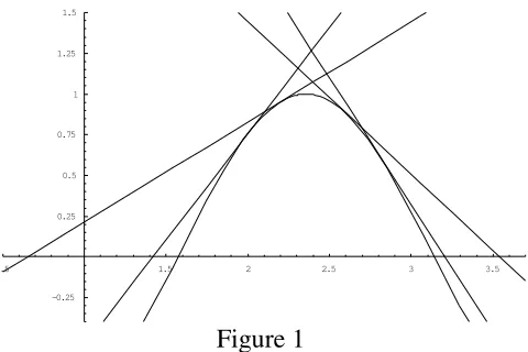
We quote, as an example, an important theorem of Analysis. It is the theorem that relates the monotonicity of a differentiable function to the sign of its first derivative. But how did we think that the monotonicity of a differentiable function is related to the sign of its derivative and we were led to stating the specific theorem? This step is a very important step for the development of the mathematical thinking of the student. The study of the motion of the tangent on the graph of a differentiable func-tion (see Figure 1) might lead to the remark that in the intervals in which the function is increasing (or decreasing), the tangent forms an acute (or obtuse) angle with the xx΄ axis. This study can be done far better with the use of the computer where the student can watch the motion of the tan-gent.

0.5 1.5 2 2.5 3 3.5

[image:21.595.179.419.314.474.2]

-0.25 0.25 0.5 0.75 1 1.25 1.5

Figure 1

The above remark leads to relating the monotonicity to the derivative. Afterwards, a more careful observation of graphs and with appropriate questions that the teacher will pose, the following conjecture could be created: if the derivative of a differentiable function is positive (or nega-tive) at an interval, then the function is strictly increasing (or strictly de-creasing) at this interval.

Use of representations for describing Mathematical deductions

(22)

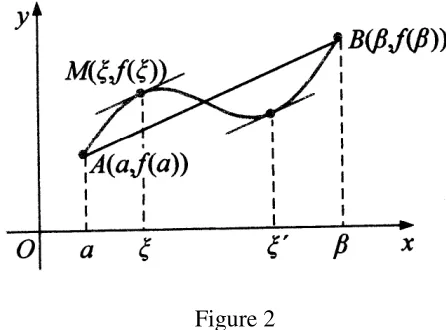
de-scription of the statement by a visual representation might help the stu-dent understand it better. A classic example is the following theorem, known as the Mean Value theorem:

“If f:[a, b] → R a function, continuous at [a, b] and differentiable at

(a,b) then there exists ξ∈ (a,b) such that f(ξ) = f b( ) f a( )

b a

−

− . ”

[image:22.595.180.403.192.357.2]

The geometrical representation of the theorem (see Figure 2) helps the student understand what the theorem actually “says”.

Figure 2

Use of representations for describing procedures and proofs

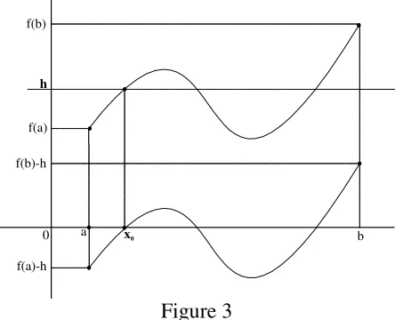
Many times, procedures or proofs seem difficult to students. They cannot understand what “they say” and so they cannot learn them. Even with procedures or proofs which students consider easy, many times students can only apply them or reproduce them only when asked. They have not understood their essence. They have not understood the essential mathe-matical idea which is hidden behind the formal presentation. The capabil-ity of describing such procedures or proofs with the use of multiple rep-resentations helps the students understand them better. An example of such a proof is the proof to the theorem of intermediate values:

“If f:[a, b] → R continuous function and f(a) < h < f(b) then there is x₀∈ (a, b) such that f(x₀) = h.”

(23)

satisfies the perquisites of Bolzano theorem. Therefore there exists x₀∈ (a, b) such that g(x₀)=0. So f(x₀)=η.

The above proof is a simple proof that does not usually create problems for many students. Yet the question remains about how many students comprehend its essence. How many understand that we make a transition of function g in order to satisfy the perquisites of Bolzano theorem? The description of the above proof with Figure 3, or ever better with the use of a computer where the motion can be shown, embodies this idea.

a _b

f(a) f(b)

h

x0

f(a)-h f(b)-h

[image:23.595.187.409.191.371.2]

0

Figure 3

In the following we describe two general frameworks which concern the teaching of concepts and theorems and which constituted the base of the planning of CalGeo activities. These frameworks are based on the princi-ple that we should try, in the teaching of Mathematics, to approach in a satisfactory point the following aims:

α) To show to students the evolution of the mathematical thinking that leads to the result.

β) To give to students the opportunity to participate actively to this evo-lution.

A framework for teaching concepts

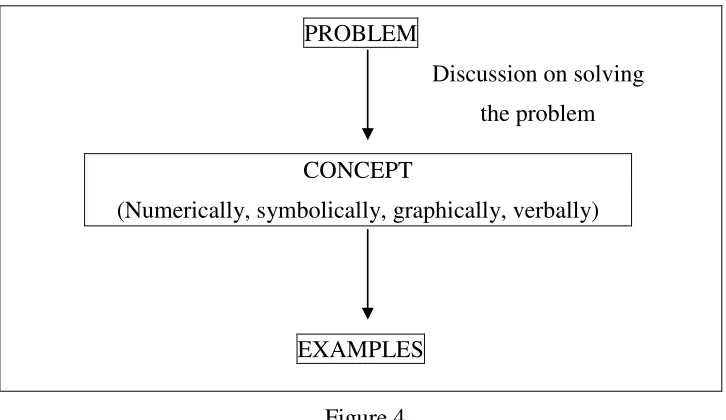
All mathematical results have, as a starting point, the solution of prob-lems. Hence when introducing a fundamental concept it is important to start with a problem that cannot be solved by the students with their ex-isting state of knowledge.

(24)

graphical and verbal descriptions help to construct the proper images and intuitions enhancing students’ understanding of the concept.

Nevertheless, since Analysis concepts are quite complicated, it is re-quired to clarify some of its aspects in order to avoid misconceptions by the students. This could be done by using appropriate examples.

The teacher, combining teaching experience and theoretical knowledge (historical, mathematical, didactical) in the particular concept, during the preparation of the course, should locate possible obstacles that students could face when encountering the new concept, and find the appropriate examples in order to overcome them.

Figure 4 shows this process in a graphical form.

PROBLEM

Discussion on solving

the problem

CONCEPT

(Numerically, symbolically, graphically, verbally)

[image:24.595.115.478.237.447.2]

EXAMPLES

Figure 4

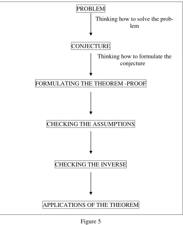
A framework for teaching theorems

When teaching a theorem, as when teaching concepts, it’s important to start with a problem that cannot be solved by the students with their ex-isting state of knowledge. The discussion regarding the solution will lead to the formation of a conjecture. Initially it may be phrased in a general form. Following that, an examination of the effectiveness of the conjec-ture is taking place. Thinking about the conjecconjec-ture leads to a more careful formation of its statement that is essentially the theorem, and also to the belief that it holds true.

(25)

Then we examine the necessity of the theorem’s assumptions.

A theorem has certain assumptions and a conclusion. The assumptions appear to be necessary since they are used in its proof. However, the fact that these assumptions are required for a proof of the theorem doesn’t mean that they are really necessary for the conclusion. Probably we could reach the same conclusion with another proof, using fewer assumptions than we already have used.

In order to be certain that each of the assumptions in a theorem’s formu-lation is necessary (that is, the conclusion of the theorem does not hold if we drop anyone of these) we have to find a counter-example that satisfies the remaining assumptions and still the theorem does not hold.

This means that there cannot be other assumptions that lead to the same conclusion.

For example, Bolzano’s theorem can be expressed as :

“Let a function f:[a, b] → R. If f is continuous and f(a)·f(b)< 0, then there is a x₀∈ (a, b) such that f(x₀) = 0.”

The two assumptions of the theorem are the continuity of f and that it’s values at its endpoints have opposite signs. In order to be sure that both assumptions are necessary, we have to find two counterexamples. One that satisfies only the continuity assumption and one that satisfies only the assumption that f(a)·f(b) < 0, so that in both cases the function is dis-continuous. This step could precede the formulation of the theorem dur-ing the thinkdur-ing process of formdur-ing the conjecture.

(26)

Sometimes the profound study of the theorem we just proved, entails new questions that could lead in turn to new results. Figure 5 depicts the aforementioned process.

PROBLEM

Thinking how to solve the prob-lem

CONJECTURE

Thinking how to formulate the conjecture

FORMULATING THE THEOREM -PROOF

CHECKING THE ASSUMPTIONS

CHECKING THE INVERSE

[image:26.595.117.481.108.554.2]

APPLICATIONS OF THE THEOREM

Figure 5

(27)

(28)

ACTIVITIES

1. INTRODUCTION TO INFINITE PROCESSES – LIMIT

OF SEQUENCES

1.1 Activity: Introduction to infinite processes

Subject of the activity

This activity is an introduction to infinite processes. This is achieved by applying the Eudoxos-Archimedes’ method of exhaustion for the calcula-tion of the area of the unit circle.

Goals of the activity:

This activity intends:

• to introduce students in a natural way to the use of infinite processes for solving problems that cannot be solved in another way.

• to help students encounter the method of exhaustion (and the idea of infinity behind it) in an environment free of algebraic calculations. • to have students acquaint anted to the interchange of representations

through the given environment where graphical and numerical repre-sentations are combined harmonically .

The rationale of the activity:

(29)

infinite process emerges naturally as a tool that allows the approach of unknown quantities no matter how close they are, by an infinite number of known ones. This idea prepares the field for the introduction of stu-dents to the limit concept at some later stage. The use of dynamic geome-try software allows not only for the graphical representation of the prob-lem, but it also eases the computation difficulties that are inherent in the calculation of the polygon areas, giving students the opportunity to focus on the infinite process

Activity and Curriculum:

(30)

1.1.1 Worksheet Analysis Introduction to Infinite Processes

PROBLEM

How can we calculate the area of the circle having radius R=1?

This is the general problem which will introduce the student to infinite processes. We expect that some of the students know the formula giving the area of the circle and may answer that the requested area is equal to π.

In this case there could be a discussion about the following questions:

• Why is this area equal to π?

• How did the formula Ε=πR2 arise?

• How can we calculate π?

In order to solve this problem, we start with three questions related to the basic area measurement knowledge

Q1. What does it mean that the area of a triangle equals 4.5?

This means that four and a half squares with sides of length 1 fit this triangle. There could be some discussion about area measurement and area measurement unit.

Q2: Find geometrical figures whose area can be measured with the previous method.

We can calculate polygon areas using the previous method.

There could be a discussion about how we can calculate the area of a polygon by diving it into smaller rectilinear shapes with easy to calculate areas.

Q3: Can we divide the circle into a certain number of figures with measurable area?

This question is equivalent to the following question: can we divide the circle into poly-gons? The polygon sides are straight line segments. The circle can not be subdivided into polygons. The negative answer leads us to the next question.

Q4: In which way is it possible to link the area under question with polygons areas?

Some discussion can arise from the students’ answers.

The target of the discussion is to be led to the idea that it is possible to find polygons whose area is either smaller or bigger than the circle area.

(That is polygons inscribed in the circle as well as polygons circumscribed around it)

Draw two squares: One inscribed in the circle and the other one circum-scribed around it.

(31)

The environment provides us with the following: We can see the circle.

The sides button controls the number n of the sides of the regular in-scribed and circumin-scribed polygons.

When the circumscribed button is pressed, the circumscribed polygon appears. Another click results to the polygon disappearance.

The inscribed button acts in a similar way.

The areas of the polygons and their difference are also displayed.

The magnification button displays a window around a predetermined cir-cle point. By enlarging magnification scale we achieve a more delicate focus.

Q5: What is the relation between the circle area Ε and the areas of these two squares?

Q6: What is the difference of these squares areas?

Using the aforementioned areas we can achieve the first estimation of the area E in question. This estimation obviously is not good enough. So we are driven to the next question.

Q7: Through which process is it possible to obtain a better approxi-mation of E?

This question is the critical point where students can pass to successive approximations. The students can probably guess that an increase in the number of sides, results to better estimations.

The instructor can prompt the students to focus on the area difference between the inner and the outer polygons as n gets bigger. The difference indicates how close the areas of the polygons and the circle are.

By constructing both the internal and the external regular pentagons we can get a better approximation of the circle area. Students may experiment with a greater number of sides.

(32)

Q8: Complete the following table:

n Inscribed n-gon area Circumscribed n-gon area

Areas difference lees or equal to 4

5 6 10 12

(18) _0.09

(23) _3.1… _3.1…

(56) 0.009

(114) _3.14… _3.14….

(177) 0.0009

(187) _3.141… _3.141…

(243)

(559) _0.00009

In this question the student fills in the empty cells of the table. The numerical results in the table intend to allow students to make some conjectures on the limits of these three sequences.

In the case of numbers such as 0.09 that are given in the table above, the students are expected to find a value of n such that the difference of the two areas is less than 0.09. 3.14… means that the number of sides is such that both the internal and external poly-gons have areas with the first two decimals equal. In the above questions students may give different answers.

Q9: Is there a step in this process in which the inscribed or the cir-cumscribed polygon has the same area with that of the circle?

To answer the question you can use the zoom-in tool and focus on a cir-cle point. By enlarging the zooming scale we can achieve better focus

Obviously no polygon can coincide with the circle.

Q10: Will this process come to an end?

Since the process doesn’t terminate it can be continued indefinitely. That is we can al-ways get polygons of more and more sides. At this point we pass to the infinite proc-esses.

Q11: Which is the number approached by the area difference?

The difference approaches 0 as the number of sides gets bigger.

(33)

We can make the difference as close to 0 as we want as long as a properly big number of sides is chosen.

Q13: How close to the circle area can we approach?

(34)

1.2 Activity: Introduction to Sequence Limit

Subject of the activity

This activity introduces the notion of Sequence Limit. Two worksheets lead the student to the definition of convergence of a null sequence. The worksheets that appear in the further exploration section lead to the defi-nition of non-zero limit.

Goals of the Activity This activity intends:

• to introduce students to the definition of the limit of sequence.

• to get students acquainted with the graphical, algebraic and numerical representations of the sequence limit

• to broaden gradually the students’ image of the definition of conver-gent sequence in order to avoid possible misconceptions (e.g every sequence converges to zero, every convergent sequence is mono-tonic).

The rationale of the activity

The problem used in the 1st worksheet is based on one of Zeno’s para-doxes. The problem has been chosen such that through the description of an infinite process the students could be introduced to the concept of se-quence convergence.

The problem of the 2nd worksheet also has a strong visual representation which becomes even stronger with the use of the dynamic geometry software. The processes which are presented in the worksheets are simi-lar and both of them can be described by the convergence of a sequence. The questions posed are chosen in a way to orient the students to the definition of the convergent sequence.

(35)

1.2.1. Worksheet Analysis Introduction to Sequence Limit I

We start with a line segment AB having a length equal to 1. A point moves from A towards B in the following way:

During the first day the point covers the interval AA1 equal to the half of

the interval AB.

During the second day the point covers the interval A1A2 equal to the half

of the interval A1B.

Keeping on this way, during the nth day it covers the interval An-1An

equal to the half of the interval An-1B.

(That is every day the point covers half of the distance left to reach B).

Q1: Will this point arrive at B?

Probably students will hold different views. Some might claim that the point will finally arrive while others that it won’t. The instructor could ask for an explanation of each opinion expressed. The goal of the discussion is to help the class reach the conclusion that the moving point will never reach point B. This can be justified by using the me-thod ad absurdum. If we suppose that it arrives at day n, this means that the n-1th day it was beyond B, let C be the point where it was on day n-1. Then on the nth day it was on the midpoint An of the interval CB, but this is different from B.

Q2: Calculate the length of the intervals AnB for n=1,2,…

1 2 1 2 1 4 1 2 ... n n A B B B A A = = =

From the above it can be claimed numerically that the moving point will never reach B because there is no n such that AnB = 0.

Q3: Let C1 be a point of AB so that C1B = 10-6.

(36)

We know from the previous question that ΑnΒ =

1

2n . So, the question is equivalent to

the following: Is there a natural number n such that 1 106 2n

−

< or 2n >106?

This is true because the set of natural numbers does not have an upper bound. So there exists a natural number nsuch that n>106 and so2n >n>106.

Some students could probably try to solve it by using the monotony of the logarithmic function. It would be better to focus on the fact that we are interested in the existence of such an n, not in the determination of a specific one. Using this as a pretext, the instruc-tor could mention the difference between proving the existence of a number n with a specific property and finding a certain numbernwith this property.

Q4: Consider the same question for points C2, C3

such that C2Β = 10-100 , C3Β = 10-1000

An argument similar to that of Q3 can show that the point will get beyond C2 and C3.

Q5: Let C be a random point between A and B. Will the moving point get beyond C?

Let ε be the length of CB. Τhe question is equivalent to the following:

Is there a natural number n such that 1

2n <ε or 1 2n

ε

> ?

This can be proved in a similar way to Q3 and Q4.

Q6: Can you describe the result you reached in question C5?

The students could postulate a proposition like the following : For any ε>0 there is a natural n such that an <ε

Q7: Complete your answer to the question Q6 in such a manner to include the information that if some day the point surpasses C then the same will hold for all the next days .

(37)

1.2.2 Worksheet Analysis Introduction to Sequence Limit II

Let ABCD be a square having side equal to 1 and K the intersection of the two diagonals.

Let A1, B1, C1 and D1 be the midpoints of KA, KB, KC and KD

respec-tively.

We construct the square A1B1C1D1.

Let A2, B2, C2 and D2 be the midpoints of KA1, KB1, KC1, and KD1

re-spectively.

We construct the square A2B2C2D2.

In general if An, Bn, Cn, Dn are the midpoints of KAn-1, KBn-1, KCn-1, and

KDn-1 respectively, we construct the square

AnBnCnDn , for n = 2, 3, …

This means that each square has its vertices on the midpoints of the line segments that connect K with the vertices of the square in the previous step .

Q1: Are there any other common points except K in the interior of all constructed squares ?

Open 1.2.1.activity.en.euc file and experiment.

The number labeled “area” represents the area En of the square

AnBnCnDn.

If needed, you can use the magnification tool.

The infinite intersection of the internal of all the squares equals {K}. This can be proved by supposing that another point L different than K belongs to the intersection and letting n grow such that the diagonal leaves L out of the square AnBnCnDn. It implies that L

doesn’t belong to the square AnBnCnDn .

Q2: Calculate the square area En of AnBnCnDn , n = 1, 2, 3, …

The student can observe that at each step the side of the square equals to the half side of the previously constructed square (Thales theorem ) and reach by induction the

conclu-sion that En =

2

1 1

(38)

Q3: Is there any of these squares with area less than 10-60?

This question can be answered both algebraically (similarly to activity 1.2.1) and by experiment on EucliDraw. The convergence of En is really fast so that the student can

experiment in EucliDraw by changing the decimal points precision .

Q4: Consider the same question for the number 10-1.000.000.

The dynamic geometry environment cannot be used in answering this question, so here becomes the need of an algebraic argument.

Q5: Let ε > 0. Is there a square, whose area is less than ε?

Questions Q3 and Q4 prepare question Q5 where there is a generalization and ε is a variable leading the student to the ε definition of a convergent sequence.

Q6: Can you find a description for the result you reached on Q5 ?

The students might write something like the following: For every ε > 0 there exists n ∈ℝ such thata_n <

ε

.

Q7: Supplement your answer on Q6 taking into account the informa-tion that if at some step the square area is less than ε, then the same holds for all the remaining steps.

(39)

Further Exploration

1. Let the sequence αn = (-1)n

n 1

, n = 1, 2, …

(i) Complete the following table:

n 1 2 3 103 116 10100

αn

(ii) Is there any real number λ being approached by the terms of αn as n

increases?

(iii) Is there a term of the sequence, so that the distance of λ from it and its successors is less than 10-6?

Consider the same question for numbers 10-100 and 10-1000 respectively.

(iv) Let ε > 0. Is there a term of the sequence, so that the distance of λ

from it and its successors is less than ε?

(v) Could you describe the conclusion you reached in question (iv) in a formal way?

2. Consider the same questions for the sequence βn =

2 n

1 n

+ +

(40)

2. FUNCTION LIMIT AT A POINT

2.1 Activity:

Introduction to function limit at a point

Content of the activity:

This activity, following the calculation of instanteous velocity, introduces function limit at a point.

The goals of the activity:

With this activity students should

• be introduced intuitively to the ε-δ definition of function limit at a point.

• connect harmonically numerical and graphical representations of the problem in order to clarify the concept of function limit.

The activity uses as a pretext an instanteous velocity problem. From eve-ryday life the students are familiar with the notion of velocity although the instantaneous velocity includes (hidden though) a limiting process. In this process the dynamic geometry software functions in two different ways. In the first part of the worksheet it provides numerical results. This enables us to avoid time consuming calculations. In the second part of the worksheet, the numerical data are represented graphically. The student can then visualize the convergence of function and move in a natural way to ε-δ definition. The use of the ε and δ zones in the dynamic geometry environment, gives the student the opportunity to handle in a dynamic way the basic parameters of the problem, in order comprehend the rela-tion between ε and δ. The green and red colors are used not as a visual effect, but as a tool that allows for the verbal representation of complex expressions.

For example the expression “All (x,f(x)) such that x∈(T−δ,T+δ) and

( ) ( , )

(41)

This activity can be taught in an hour lesson, as an introduction to the definition of the function limit concept.

(42)

2.1.1 Worksheet Analysis

Introduction to function limit at a point

PROBLEM A camera has recorded a 100m race.

How could the camera’s recording assist in calculating a runner’s velocity at T=6sec?

• Open activity2.1.euc EucliDraw file. In this environment we can get the camera’s recordings.

• When changing the values of t, the values of s(t), that represent the distance the runner has covered up to t, also change.

• t can approach T from less and greater values. • Display the average velocity.

The yellow box displays the average velocitys T( ) s t( )

T t

−

− in the interval defined by t and T.

Q1: Fill the empty cells in the following table.

t s T( ) s t( )

T t

− −

t s T( ) s t( )

T t

− −

4 8

5 7

5.5 6.5

5.8 6.3

5.9 6.1

5.93 6.07

5.95 6.03

5.99 6.01

5.995 6.005

5.999 6.001

5.9999 6.0001

5.99999 6.00001

There can be conversation on the notion of average velocity.

(43)

bigger numbers. This is due to the fact that the quantity T-t equals zero and the average velocity has no meaning since denominator is zero.

Q1: Which number does the average velocity approach as t ap-proaches T=6sec?

As t approaches T from both greater and less values, we can observe that the average velocity approaches 10m/sec. It’s useful to make clear to the students that t can be arbi-trarily close, but never equal, to T.

Q2: What is the runner’s velocity at T=6sec?

• Display the Average velocity Function U(t) in EucliDraw and con-firm your findings graphically.

• Display the ε-zone in the EucliDraw file. The points in the ε-zone have ordinate that is bigger than L-ε and less than L+ε.

• Move t so that (t,U(t)) lies inside the epsilon zone, and observe the values of the average velocity.

Although we have determined the limit, we now show the function and try to see the convergence on the graph.

Q3: For which values of t is the point (t,U(t)) inside the ε=0.8 zone?

You may have some assistance on answering this question by displaying the delta zone. Points inside the δ-zone have abscissa bigger than T-δ and smaller than T+δ. Points simultaneously inside epsilon and delta zones are coloured in green. Points outside the epsilon zone are coloured in red.

The student can experiment by moving t and observing the change of U(t).

Q4: Try to find a δ such that no points of the graph lie in the red area.

If we have δ equal to 0.7 we get what we wanted.

Q5: Decrease ε to 0.5 and find a δ such that the points (t,U(t)) do not lie inside the red area.

e.g δ=0.4.

Q6: If ε=0.05 can you find such a δ?

You can display the magnification window. It can assist you in viewing inside a small area around (T,L).

e.g δ=0.05.

Q7: If ε gets less and less, will we be always able to find a suitable δ

(44)

The students can experiment with less and less values of ε and conclude that they will always be able to find a δ.

Q8: Fill in the blank with a suitable colour in the following statement in order to express the conclusion of Q7.

“For every ε>0 we can find a δ>0 such that the function does not lie in the ……red………. area.”

We need to pay attention to this proposition because it may lead students to a misunder-standing. The student may believe that even if the function was defined at point T then the value L=f(T) should not lie in the red area. This activity doesn’t make clear that what interests us is not what happens at T but only what happens around T.

In some further activity it should be good to clarify that when examining the existence of a limit at a point, the value of the function (in case it exists) could lie inside the red area.

Q9: Fill in the blanks so that the following statement bears the same conclusion as Q7

The ………..U(t) ………. can be arbitrarily close to …………..L………. as long as the ………t……….are close enough to ………T……….. and different than …..T………..

Q10: Try to formulate the conclusion of Q7 using mathematical symbols

This is the most critical step and a conversation may take place taking into account the students’ answers. The teacher can remind his/her students that the distance between two numbers equals the absolute value of their difference. The goal of this question is to give the ε-δ definition of the limit of a function at a point.

(45)

3. CONTINUITY OF A FUNCTION AT A POINT

3.1 Activity: Introduction to continuity of a function at a point

Content of the activity:

This activity introduces the students to the notion of continuity (and dis-continuity) of a function at a point. Through the study of a problem, stu-dents are leaded to an informal verbal representation of the continuity definition, in a way that it enables a smooth passing to the algebraic rep-resentation of the ε-δ definition.

Goals of the activity: This activity intends:

• To introduce students intuitively to the ε-δ definition.

• To familiarize students to the “find a suitable δ whenever given an ε” kind of process, within a dynamic geometry environment, free of al-gebraic manipulation.

• To connect different representations of the concept of continuity. • To realize the ε-δ definition's failure as a jump on the graph.

The ε-δ definition of continuity presents serious difficulties. Through this activity we seek to introduce students to continuity of function at a point, in an intuitive way free of algebraic manipulations.

The activity is divided into three steps. In the first step, through a prob-lem, some concrete values of epsilon are given and the student is asked to find the corresponding δ. In the second step ε becomes a parameter. In the third step the student connects discontinuity to the existence of a jump in the graph. In each step the questions are first implemented graphically and then algebraically.

(46)

idea of continuity or –under suitable adjustment - can be also used as an intuitive introduction to the main idea of continuity

(47)

3.1 Worksheet Analysis

Introduction to continuity of a function at a point

FIRST STEP

A chemical and health care corporation is about to produce a new antibi-otic pill which will be able to cure a certain disease.

It is known that the pill should contain 3gr in order to provide the patient with the right dose of medicine.

The function f x( )= x+ −1 1gives the amount ( )f x of the antibiotic which is detected in the blood, when a patient gets a pill with xmgr of the substance.

According to current research results, if the antibiotic detected in blood is equal or less than 0.8gr, there will be no effect on the patient’s health and if it is more than 1.2gr the patient is in danger due to overdose.

Q1: Which amount of medicine is presumably detected in the pa-tient’s blood?

(3) 1

f =

Q2: Which is the allowed error ε of divergence of the detected amount of medicine from the ideal value, such that the pills stay safe and effective?

The number ε=0.2 sets a boundary (1 0.2 ,1 0.2)− + =(0.8,1.2)on the ac-cepted quantities of antibiotic around f(3)=1. We will call ε the allowed error.

Some questions that familiarise students with the allowed error could be useful since epsilon plays a vital role throughout the activity. It is very useful to introduce the terms “allowed error” and “precision” in our language as soon as possible.

The machine available to the corporation that produces pills of t=3gr has an accuracy level adjusted to δ=1.1

(48)

Q3: Is the machine suitably adjusted to produce safe and effective pills?

• Open EucliDraw file 3.1.1a.activity.gr.euc and try to answer ques-tion E3 using it.

• In this environment we get the graph of f(x). By changing ε we can alter the allowed error, and by changing δ we can alter machine’s ac-curacy.

• The magnification window allows us to focus in a neighbourhood of point (3,1).

The student is expected to observe that there are some parts of the graph which lie in-side the delta zone, but outin-side the epsilon zone. If we set the machine to produce pills, some of them will be ineffective and some dangerous.

The machine can be adjusted to another accuracy level.

Q4: Can the machine be adjusted in order to produce pills within the allowed error?

We expect the students to change delta in order to fix the problem of the previous ques-tion. The students should work from both sides in order to find a delta of about 0.8. Some discussion may be held in order to emphasize that δ is not unique.

Every δ less than the one already found can work fine.

Another point that needs extra attention is the fact that we are not interested in finding a better δ.

The results of a new research indicated that the error level should be re-duced to ε=0.1.

Q5: Is there any problem with this change in pill production? Does the accuracy level have to be adjusted anew?

Each student's answer depends on which δ has given in the preceding question.

For example if a student has given δ=0.8 before, the machine after the change of ε does not work right. If a student's δ was 0.2, then the machine still does not have a problem. A δ of 0.3 or less does work.

SECOND STEP

(49)

Open activity3.1.1.euc file and check whether we can always find an adequate δ>0, as ε gets smaller and smaller. Experiment graphically. Display the Red/Green region and describe what it means for the function graph to lay in the green, red or white region.

This question offers the student the opportunity for a transition from a visual representa-tion to a verbal one.

The green region represents the allowed (x,f(x)).

Algebraically, the green region is the set of those points (x,f(x)) of the plane for which, |x-5|<δ and |f(x)-f(5)|<ε

When some part of the function lies in the red region then there is a problem in the pill production. The machine is programmed in such a way, that it may produce pills which are ineffective (red part bellow the green region), or harmful (red part above the green region).

No point in the white region can be produced by the current state of the machine.

If necessary, use the magnification window.

In this question, the student plays an ε-δ game giving less and less epsi-lons. When ε lessens enough the zones are indistinguishable, so the inter-est moves to the magnification window.

Q2: In each of the following sentences, fill in the blanks with the cor-rect colours:

a. Whenever we are given an ε, we can find a δ,

such that the function does not lie in the ...red... region.

b. For every ε we can find a δ such that for every x in the accuracy limits of the machine, (x,f(x)) lies in the ...green... region.

Q3: Write sentence b, replacing the colours with algebraic relations.

The teacher initially leads the students in a verbal description of the result like : “For every arithmetic value of the error, there is a machine accuracy so that if x lies inside the bounds of the allowed precision, f(x) lies inside the bounds of the allowed error”.

Hereupon he can ask them to demonstrate the description above with the use of mathe-matical symbols. That is

“For every ε we can find a δ such that for every x∈(3−δ, 3+δ) we have:

(1 ,

) )

( 1

(50)

Or

For every ε we can find a δ such that for every x such that |x−3 |<δ, we have | f x( ) 1 |− <ε.

Under suitable circumstances the last proposition can drive to the introduction of ε-δ

definition of continuity in the case of a random function.

THIRD STEP

Another research shows that the formula given by the function above which gives the quantity of drug traced in blood works well for values less than 3mgr. When values of x exceed or equal 3 it shows 0.06mgr less than the real amount detected in blood.

Q1. Find out the formula of the new function that gives the real quantity of drug detected in blood, taking into account the results of the last research.

1 1 , 3

( )

... , 3

x x

g x

x

 _{+ −} _<



=

≥



The second branch should be x+ −1 0.94

Q2: Can the machine be adjusted properly to produce effective and safe pills?

Which δ should work for ε=0.1?

E.g. δ=0.1 works.

Open activity3.1.2.euc file

Give your answer by giving suitable values δ. If needed use the magnification window.

ε is chosen in a way that a δ can be found.

Q3: What will happen if ε is reduced to 0.06? Can you find an ade-quate δ?

No δ can make the machine produce only effective pills since whenever a pill is less than 3mgr the quantity detected will be ineffective.

(51)

This question may lead the class to some very interesting discussion.

Some idea that can lead to the discontinuity concept is the fact that the gap which exists in the graph of f(x) is what causes the failure in finding δ, as long as the points g(x) around 3 appear distanced from each other.

Q5. In each of the following sentences, fill in the blanks with the cor-rect colours:

a. For a given an ε, no δ could prevent the function from lying in the ...red... region.

b. There is an ε, such that for every δ, there is an x in the accuracy field of the machine such that (x,g(x)) lies in the ...red... region.

Q6. Write sentence Q5b using algebraic relationships instead of col-ours.

There is an ε such that for every δ, there is anx∈(3−δ, 3+δ), such that

(1 ,

) )

( 1

g x ∉ −ε +ε . Or There is an ε such that for every δ there is an x such that |x−3 |<δ , for which we have | ( ) 1 |g x − ≥ε.

(52)

4. DERIVATIVE

4.1 Activity: The notion of derivative and the tangent

Content of the activity

This activity aims to introduce the students to the notion of the derivative of a function at a point x₀through the geometric representation of the

tangent line of the curve at the point ( 0

x , f(x₀)). In designing this activity students’ previous knowledge concerning the tangent of the circle, was taken into account.

Goals of the Activity:

Through this activity we aim students:

• Generalise their previous knowledge concerning the tangent line grounded in the context of Euclidean Geometry, to other more gen-eral types of curves.

• Be introduced to the notion of the tangent line at point (

x

₀, f(

x

₀)), as the linear approximation of the curve at this point.

• Be introduced to the notion of derivative at a point

x

₀.

• Understand the geometric representation of the derivative at a point

0

x

as the slope of the tangent line at the point (

x

₀, f(

x

₀)).

• Connect the symbolic representation of the derivative of a function at a point with the geometric one.

• Recognise from the curve of a function at which points the function is differentiable.

The rationale of the Activity:

Teaching calculus using dynamic geometric tools

CALGEO

Teaching Calculus using

Dynamic Geometric Tools

Teaching Calculus

Using

Dynamic Geometric Tools

CONTENTS

PREFACE

INTRODUCTION

DESCRIPTION OF

CALGEO

PROJECT

THE TEACHING OF ANALYSIS

ACTIVITIES

1. INTRODUCTION TO INFINITE PROCESSES – LIMIT

OF SEQUENCES

1.1 Activity: Introduction to infinite processes

1.2 Activity: Introduction to Sequence Limit

ε

2. FUNCTION LIMIT AT A POINT

2.1 Activity:

Introduction to function limit at a point

3. CONTINUITY OF A FUNCTION AT A POINT

3.1 Activity: Introduction to continuity of a function at a point

4. DERIVATIVE

4.1 Activity: The notion of derivative and the tangent

x

x

x

x

x

x