Holistic User Context Aware Recommender Algorithm

(1)

Research Article

Holistic User Context-Aware Recommender Algorithm

Tatenda D. Kavu ,

1

Kudakwashe Dube ,

2

and Peter G. Raeth

3 1_{Computer Science Dept, University of Zimbabwe Harare, Harare, Zimbabwe}

2_{School of Fundamental Sciences, Massey University Palmerston North, Palmerston North, New Zealand}

3_{University of Gondar, Gondar, Ethiopia}

Correspondence should be addressed to Kudakwashe Dube; [email protected]

Received 29 January 2019; Revised 5 June 2019; Accepted 14 July 2019; Published 29 September 2019

Academic Editor: Rosa M. Benito

Copyright © 2019 Tatenda D. Kavu et al. This is an open access article distributed under the Creative Commons Attribution License, which permits unrestricted use, distribution, and reproduction in any medium, provided the original work is properly cited.

Existing recommender algorithms lack dynamism, human focus, and serendipitous recommendations. The literature indicates that the context of a user influences user decisions, and when incorporated in recommender systems (RSs), novel and ser-endipitous recommendations can be realized. This article shows that social, cultural, psychological, and economic contexts of a user influence user traits or decisions. The article demonstrates a novel approach of incorporating holistic user context-aware knowledge in an algorithm to solve the highlighted problems. Web content mining and collaborative filtering approaches were used to develop a holistic user context-aware (HUC) algorithm. The algorithm was evaluated on a social network using online experimental evaluations. The algorithm demonstrated dynamism, novelty, and serendipity with an average of 84% novelty and 85% serendipity.

1. Introduction

Research in recommender systems research has recently diverted attention to context-aware recommender systems (CARS) since incorporating contextual information in rec-ommender systems is an eﬀective approach to create more accurate and relevant recommendations [1]. Recommender algorithms are generally limited to coping up with the dy-namics of user preferences [2, 3]. In current recommender systems (RSs), adaptive learning is basically derived from computing neighbourhood of a user from ratings using distance functions such as Pearson correlation function and Euclidean distance function. Therefore, adaptation will be mainly the by-product of the neighbourhood computation. If a user rates something new, his/her neighbourhood changes, and as a result, the recommendations got by this user are likely to change. This is the type of adaptive recommendation which is experienced in current recommendation algorithms. However, preferences inferred from user actions only are inadequate to deduce sound user-centric predictions [4].

Recommender algorithms are found lagging behind the dynamics of user preferences, resulting in lack of sound

dynamic, novel, and serendipitous recommendations [5]. Moreover, the incorporated contexts in CARS are not enough for tailoring personalized services to users. One or two contexts are only incorporated in recommender sys-tems, and these are not enough to represent users’ interests or preferences [6]. The literature indicates that recom-mender algorithms lack signiﬁcant novel and serendipitous recommendations [7, 8].

To address the identified challenges, an investigation was carried out and it was found that recommender algorithms are biased significantly towards system-centric factors such as accuracy, diversity, and scalability [9]. There is a lack of in-corporation of knowledge from these user-centric factors (user experience, user decision-making processes, and user interaction) [10]. Therefore, this article presents a unique method of incorporating users’ decision-making knowledge into a recommender algorithm. The context-aware recom-mender algorithm uses the holistic contextual user profile in the form of social, cultural, psychological, and economic profile, together with items associated with the user to offer recommendations. When tested online, the algorithm proved to offer dynamic, novel, and serendipitous recommendations

(2)

to any user as compared to any algorithm that uses ratings and rated items.

The main contribution of this work is the contextual modelling of the holistic user contextual proﬁle in order to provide dynamic, novel, and serendipitous recommenda-tions. The approach brings the beneﬁt of satisfaction to the users of the recommender system. The rest of the paper is organized as follows: Section 2 shows related work, Section 3 shows the materials used and the theory behind the rec-ommendation approach, Section 4 demonstrates the ex-perimental setup, Section 5 shows the results, and Section 6 discusses the results. Finally, Section 7 summarizes and provides future directions.

2. Related Work

Contextualization is viewed as a paradigm for building intelligent systems that can better predict and anticipate the needs of users and acts more eﬃciently in response to their behavior. The incorporation of contextual information about the user in the recommendation process has attracted major interest [11]. Contextual information matters in RSs, and it is important to take this information into account when providing recommendations [12].

Contextual information/features of a user such as time and location are quite important in making novel and serendipitous recommendations [1, 7, 13, 14]. Modelling the contextual information about a user enables the recom-mendation engine to provide more reasonable recommen-dations for users [13, 15], and context adaptation is one major goal of session-aware recommendation engines [16]. It is a well-known fact from decision science that a decision made speaks a lot especially about the decision-maker’s values [17]. If a user chooses an item or prefers an item, people with the same values with this particular user are likely to be interested in the same items [18]. Since users’ preferences are likely to be similar to, or influenced by friends [19]. Users first identify the need of an item and then search for it and evaluate alternatives from the search before making a purchase [20]. Understanding users of RSs is the key issue for better recommendations, and users can be advised at the right place and at the right time with the right message [21]. The researchers of this article found from the literature that users are influenced by significant factors such as economic status, psychological status (e.g., mood), cul-tural values, and social status when choosing an item or a service [7, 21]. In summary, these are the factors that spell all conceptual issues that explain theoretical derivations of user preferences.

There are algorithms that incorporate time in the rec-ommendation engines due to the fact that, in some cir-cumstances, a recommendation that is relevant in the morning context may not be relevant in the evening and vice versa [7, 22]. In clothing industry, clothes needed during summer and winter may be diﬀerent. Time can be aggre-gated such that it can be classiﬁed in daily periods for in-stance {morning, afternoon, evening} or seasonal periods such as {summer, winter, spring, autumn} or event periods such as {Christmas, new year, school reopening, etc.} [7, 21].

Recently RSs have been designed which incorporate time [2, 23]; however, an algorithm that focuses on the holistic approach of incorporating important decision-making factors in the context of {social, cultural, psychological, economic} factors has not been investigated or imple-mented. Generally, recommendation algorithms work with a general assumption that recent ratings are more important than older ratings [1, 22]. Users generally select content or items based on current desires or preferences at the time of selection. Such desires or preferences, however, often ﬂuc-tuate over time [1, 19, 24].

Most of the work on CARS has been conceptual. Col-lection of big data for incorporation in CARS is still another major challenge that needs to be tackled [11]. Overall, the ﬁeld of CARS is a relatively new and under explored area of research, and much more work is needed to investigate it comprehensively [12].

Vargas [8] did a phenomenal series of researches and proved that there was no significant groundwork that had been performed before on novelty. He came up with a unified framework for novelty and diversity coming from an integration of different mathematical models that describe novelty and diversity. He built the framework on the ar-gument that novelty and diversity are inextricably in-terrelated. It is quite recognizable that computation of novel recommendations is done during the time of ranking the recommended list. The recommended list is shuffled to make sure that the final list is novel and diverse.

Lee and Lee [9] also proposed an algorithm to provide novel recommendations whereby a graph-based recommender al-gorithm was developed that uses positively rated items in users’ proﬁles to construct a highly connected undirected graph. Items were represented as nodes and positive correlations as edges. Using the concept of entropy and the linked items in the graph, the proposed algorithm was able to ﬁnd recommendations that were both novel and relevant.

The strategy of computing novel recommendations seems to be satisfactory from the status quo, but the argument still exists that serendipity is even more beneﬁcial than novelty because it creates new preferences to the user thereby driving a user to make decisions in favor of the RS [7, 19, 25, 26] argues that new methods of extracting implicit information about users from their daily activities can be used to realize novel and serendipitous recommendations. Alternative methods can be explored to rank and recommend items to users by considering several criteria [13, 27, 28, 29], and that is the path taken by this article.

3. Materials and Methods

3.1. Relevant Theory

(3)

status (which include type of profession, social class, and possessions). Therefore, given that a recommender algo-rithm has access to user’s contextual information, that al-gorithm should at least be able to give reasonable, unique novel recommendations to that user.

RS users are naturally found in different contexts [22, 30]. Users’ tastes or behaviors can be affected by many contextual circumstances of the user, for instance, social life, mood, cultural background, economic status, location, and factors such as time (weekdays, weekends, and holidays) [22]. The geographical location of a user can have a sig-nificant influence on his/her preferences in clothing or food [31]. From an extensive review of the literature, the re-searchers found that the user contextual phenomenon can be classified into four classes. These classes are social, cultural, psychological, and economic status. If a user is in a certain social or cultural context, that user has particular needs. The same applies when a user is in a certain mood (psychological status), that user will like or dislike certain items [24]. If a user is in a certain economic status or context, that user is able or not able to afford certain items. It also entails that if the user’s social status or economic status changes, he/she will have different preferences or tastes. Therefore, a rec-ommender algorithm must take all the four contextual classes into consideration to offer dynamic, novel, and serendipitous recommendations to users.

3.1.2. Principles behind Computations. The main principle behind the computation of the holistic user context-aware (HUC) algorithm is that users in the same context (social, cultural, psychological, and economic status) are likely to have the same taste or similar set of preferences. There are similarity functions such as Jaccard similarity function, Pearson correlation function, and Euclidean distance function which can be used to ﬁnd the contextual similarity of users, using their proﬁles. Table 1 shows the comparison of these similarity measure functions.

Jaccard was used in this article because of the nature of the input data to the HUC algorithm. Jaccard is a simple statistic used for comparing the similarity and diversity of sample sets. It is a similarity distance measure similar to other methods of measuring similarity such as Euclidean distance, Pearson’s correlation coefficient, and cosine similarity function. Its main advantage in this case is that it is best applicable in measuring the similarity of finite sets. Profiles can be converted into sets and are easily compared to find out similar profiles. The Jaccard index is a measure of similarity between sets and produces a value between 0 and 1.0 inclusive. It was introduced by Jaccard, the late professor of botany [32]. Many developers of rec-ommender systems have used the Jaccard similarity to find the similarity between different types of sets especially in content-based recommender systems where it is used to measure the similarity of two documents [31]. Some of the published work where Jaccard was used include [32, 33] and [32, 34–37].

3.1.3. Graphical Representation of the Computational Theory.

Similarity computation can be performed to ﬁnd a link or similarity between user proﬁles. Using the graph theory, a

graph is deﬁned as an ordered triple V(G), E(G), andψG.

Where V(G) is a nonempty set of vertices (where vertices are user proﬁles in this case), E(G) is a set of edges (edges are a

representation of similarities), and ψG which is associated

with each edge of G as an unordered pair of (not necessarily

distinct) vertices of G.ψG is therefore the Jaccard similarity

coeﬃcient value that depicts the similarity between two

vertices. If eis an edge andu andvare vertices such that

ψG(e)�uv�0.9, then e is said to be joining u and v; 0.9

shows the similarity value of the two vertices and depicts that

uandvare very similar.

Therefore:

G�(V(G), E(G),ψG)

V(G)�user1, user2, user3, user4, user5, user6, user7,

user8

E(G)�e1,e2,e3,e4,e5,e6,e7

Suppose at some unique timet,ψG is depicted as follows:

ψG(e1)�user1 user2�0.8,

ψG(e7)�user4 user8�0.6

If user proﬁles have a similarity with a range of 0.5–1, it means that these users are similar. In other words, they are in related contexts and are likely to be interested in the same items. Therefore, from Figure 1, user 4 will be rec-ommended items clicked/rated (that is actioned) by users 7 and 8. Looking at the graph, we can conclude that user 8 and user 7 are likely to be similar since they are both similar to user 4. Given that they have recent actions performed on the system according to the HUC algorithm, both are likely to be recommended items actioned by user 4. If the RS is deployed on a social network, then user 8 is likely to be recommended user 7 as a potential friend or a potential client.

3.1.4. Computational Efficiency. Novelty and serendipity are to a greater extent realized when using active profiles to compute neighbourhoods. Given that there are more than a million active users, it becomes computationally expensive to calculate the Jaccard similarity between the concerned users with the rest of the active users. This means that the efficiency and robustness of the algorithm are affected. Therefore, there is a need for a robust method that can be used to trim down the number of active users needed during similarity computation. We deliberated on

classi-ﬁcation and clustering algorithms such as k-means

clus-tering, k-nn nearest neighbour, and decision trees.

(4)

profiles using decision trees. When a new user comes in, he/ she will be placed in a specific class, and from that class, another computation will be done to compute his/her neighbourhood using the Jaccard similarity metric. This method reduces the computational time significantly. Moreover, classes will be changing systematically since the user profile will be updated by the user’s activities. When a user profile changes, the user is migrated to another class of similar profiles. This approach gives rise to dynamic recommendations.

(1) Classiﬁcation using the ID3 Decision Tree. Using the

ID3(Iterative Dichotomiser 3) version of a decision tree

designed by Ross Quinlan, we start by calculating en-tropy, which is a statistical metric that measures the impurity of the data set. Given a set S of user proﬁles, which contains two classes: positive (meaning user did the anticipated action) and negative (meaning did not do the anticipated action), entropy with respect to this Boolean classiﬁcation is

entropy(S) � −p(positive)log 2p(positive)

− p(negative)log 2p(negative), (1)

whereppositive is the probability of positive examples in S

andpnegative is the probability of negative examples in S.

Information gain is the measure of the expected re-duction in entropy. It decides which among the attributes of

the concerned user’s profile (the user that we want to classify) goes into a decision node (which attribute can be used to split the set). To minimize the decision tree depth, the attribute with the most entropy reduction is the best choice. The subset returned by a splitting decision must have a size of greater or equal to 50 profiles, and when the size is lower than 50, the splitting process stops and the user of concern is then classified:

Gain(n) �Entropy(n)−([weightedaverage]∗entropy),

Gain(S,A) �Entropy(S)Oentropy

− 􏽘

x∈values (A)􏼌􏼌􏼌􏼌Sv􏼌􏼌􏼌􏼌

|S| ∗Entropy Sv􏼁,

S�Each valuevof all possible values of attribute A,

Sv�Subset of S for which attribute A has valuev,

Sv

􏼌􏼌􏼌

􏼌 􏼌􏼌􏼌􏼌�Number of elements in Sv,

|S| �Number of elements in S.

(2)

Given that on an e-commerce platform at a certain moment, a user was about to be classiﬁed into a certain class

which shares the same attributes as him using the ID3

de-cision tree. A set of user proﬁles together with their transactional history (whether they have bought or not on the e-commerce platform) was retrieved from the platform as shown in Table 2. These very short proﬁles will be used to

demonstrate how the ID3decision tree can compute the class

of useri. In column action, 1 represents that the user bought

something, 0 represents that the user did not buy anything. The attributes maybe {age range, gender, location, hometown, time period, profession}, and they can have the following values:

age range�{20−25, 25−30, 30−35, 35−40}

gender�F, M

location�{harare, gweru, bindura, mutoko, bulawayo}

hometown�{chinhoyi, gweru, masvingo, mutoko,

bindura}

time period�{morning, afternoon, evening}

profession�{law, engineering, education, indigenous,

health, student}

We need to ﬁnd which attribute will be the ﬁrst decision node in the decision tree:

Table1: Comparison of similarity measure metric functions.

Jaccard similarity function Euclidean distance function Pearson correlation function Measuring similarity of ﬁnite sets Measure distance between data points Measure linear correlation Can work with strings Work with vectors of real numbers Corelational real numbers Easy to work with social media proﬁles Computationally expensive, when dealing with social

media data Weak on complex relationships Best for content-based recommendations Good for collaborative ﬁltering algorithms Good for collaborative ﬁltering

0.8

0.1

0.5 0.3

0.7

user1 user2

user4

user7

user8 user3

user5

user6 0.6

0.5

(5)

Entropy(S) � − 7

9

􏼒 􏼓log 2 7

9

􏼒 􏼓− 2

9

􏼒 􏼓log 2 2

9

􏼒 􏼓�0.764,

Gain(S, gender) �Entropy(S) − 5

9

􏼒 􏼓∗Entropy(SF)

− 4

9

􏼒 􏼓∗Entropy(SM)

�0.764− 5

9

􏼒 􏼓∗0.7219− 4

9

􏼒 􏼓∗0.811

�0.723,

Entropy(SF) � − 4

5

􏼒 􏼓∗log 2 4

5

􏼒 􏼓− 1

5

􏼒 􏼓∗log 2 1

5

􏼒 􏼓

� 0.7219,

Entropy(SM) � − 3

4

􏼒 􏼓∗log 2 3

4

􏼒 􏼓− 1

4

􏼒 􏼓∗log 2 1

4

􏼒 􏼓

�0.811.

(3)

Looking at the scenario above, information gain of other attributes is less than 0.723; therefore, gender will be

used as the ﬁrst decision node. Useriend up in the class of

males who made their transactions in the morning.

Therefore, the minimum possible class size of useriwill be

returned to other modules of the HUC algorithm for

further computation. As shown in Figure 2, useriwill be in

the same class as user4. Therefore, a similarity function

will be called to compute the similarity between useriand

user4.

When a user’s context changes either in the form of social, cultural, psychological, or economic context, that user’s friends (neighbourhood) change as well. Therefore, the user’s predicted preferences will be derived from the user’s recent context or proﬁle. Thus, the HUC algorithm will not be stuck with the user’s historical preferences. The change of neighbourhood will be an outcome of the new similarity computation. Novel and serendipitous recommendations will be a product of computing other recommendations from recent acted items within the neighbourhood of the concerned user.

3.2. The HUC Recommender Algorithm

Vectors:

P_i�tuple (s,c,p, e) (a proﬁle for useri)

s�tuple (a₁, . . ., a₇), where ai is a social attribute

(relationship status, age range, gender, education, likes, political aﬃliation, social status)

c�tuple (c₁, . . ., c₅), wherec_i is a cultural attribute

(religion, current location, hometown, timezone/time period, language)

p�tuple (p₁, . . ., p₄), where p_i is a psychological

attribute (birthday, friends birthday, movies, up-coming events)

e�tuple (e₁,. . .,e₅), wheree_iis an economic attribute

(currency, work history, profession, residential category)

Sets:

I�{x: x is an item/product}

I_r�{x:x∈I AND recommended toP_u}

U�{x:x�P_u, whereP_uis a proﬁle for useru}

O�{x:x∈U_o, where o is an old user proﬁle}

R�{x:x∈UAND xis an active user}

N�{x:x∈U_n, where n is a new user proﬁle}

M�{x:x∈RAND Similarity (xi, xj) ≥n, where n is

0.5,∀i, j}

Check if user u has previously expressed interest in

producti:x∈Boolean, isActive (u,i)�x, u∈UANDi∈I

(i) Derivative expressions:

R⊆U, U�O∪N, andM⊆R

Algorithm 1 computes recommendations to users, and it starts by passing existing users to Algorithm 2. Algorithm 2 starts by computing active users from the existing/old users and then

comes up with similar users to the concerned userufrom active

users, and it retains a list of users who are similar to the con-cerned user. Algorithm 1 then computes frequent items actioned by similar users by calling Algorithm 3. These frequent sets of

items are the ones recommended to the useru. Time complexity

for the ComputeRecommendations algorithm is mainly de-termined by the time complexity of Algorithms 2 and 3.

Algorithm 2 computes the similarity of proﬁles. Given a list of proﬁles, it computes the similarity of the given list in relation to a particular user. The main algorithm to be called is the Jaccard similarity algorithm, which does the un-derlying work of computing similarity. The time complexity of Algorithm 2 is shown below:

n�|O|,m�|R|, T(computeProﬁleClassSet(u, O)),

T(Jac-cardSimilarity(m, u))

T(R)�n∗1, T(M)�m∗n2

T(ComputeSimilarProﬁle)�n+m∗n2

O(n+ mn∗2)≈O(mn2)

Algorithm 3 uses association rule mining (apriori) to compute frequent sets. The main task of this algorithm is to come up with a set of items which are frequently actioned by similar users. The actions might be searching, clicking, rating, etc. Its time complexity is illustrated as follows.

Table2: A short blueprint of user proﬁles.

User Age range Gender Time period Action

1 20–25 F Morning 1

2 25–30 F Afternoon 1

3 20–25 M Evening 0

4 30–35 M Morning 1

6 35–40 M Afternoon 1

7 35–40 F Morning 1

(6)

M

F

Gain(S, time_period) == max while(len(S) > 50)

continue

Gain(S, time_period) == max while(len(S) > 50)

continue Gain(S, gender) == max

while(len(S) > 50) continue

Morning Afternoon Evening Morning Afternoon Evening

user1, user7

useri, user4 user6 user2, user8

len(S) ≤ 50

Figure2: A snippet of the decision tree.

(1) ComputeRecommendations (2) INPUT:

(3)I(set of items actioned byM) (4)u(proﬁle of user)

(5) OUTPUT:Ir(items recommended tou) (6) Begin

(7) M⟵(ComputeSimilarProﬁle (u,O))

(8) Items_on_demand⟵ComputeItemsActionedbySimilarProﬁle (M,I,u) (9) Ir⟵I∪Items_on_demand

(10) returnIr (11) End

ALGORITHM 1: ComputeRecommendations.

(1) ComputeSimilarProfile (2) INPUT:u(profile of user) (3) O (set of old profiles)

(4) OUTPUT:M(set of proﬁles similar to proﬁleu) (5) Begin

(6) C⟵computeProﬁleClassSet(u,O) (7) R⟵{r:r∈CandisActive(r,I)}

(8) k⟵0.5;(Jaccard coeﬃcient threshold for highly similar proﬁles) (9) M⟵{m:m∈RANDJaccardSimilarity(m,u)≥k,∀m} (10) returnM

(11) End

ALGORITHM2: ComputeSimilarProﬁle.

(1) ComputeItemsActionedbySimilarProfile (2) INPUT:M(set of profiles similar to profile u) (3) u(profile of user)

(4) I(set of items actioned byM) (5) OUTPUT:It(set of items actioned byT) (6) Begin

(7) freqSet⟵Apriori(M,I,u)

(8) T⟵{t: (t∈MAND (isActive(t, freqSet))} (9) It⟵{i:i∈(I UfreqSet) AND isActive(T,i)} (10) returnIt

(11) End

(7)

Time complexity for the ComputeItemsActionedbySi-milarProﬁle algorithm is as follows:

n�|freqset|,m�|T|,z�|M|,p�|I|, g�|It|,k�constant

T(freqSet)�2p, T(T)�z+ 1(2p), T(I_t)�p+ 1 +n+p

T(ComputeItemsActionedbySimilarProﬁle)�p+ 1 +n+

p+z+ 1(2p) + 2p

O(p+ 1 +n+p+z+ 1(2p) + 2p)≈O(n)

Algorithm 4 in particular is responsible for reducing the list of old users with recent events/actions. This algorithm

implements the ID3 decision tree. Given that on a platform

there are a million active users, Algorithm 4 will trim down the number of active users to a very small list of maybe up to 50 users. Algorithm 2 will then compute similar users from this new list. This method reduces the time for extracting similar users signiﬁcantly. Operations such as this can be run in the background so that they do not disturb user interaction.

The time complexity of the classiﬁcation algorithm (computeProﬁleClassSet algorithm) is as follows:

n�|O|, m�|Go|, d�|Od|, k�constant, e�| A |,

T(Entropy(o)�1,

T(

􏽐|Vo|

x∈V_o(|Ox|/|Oai|∗Entropy(Ox))

})

T(Go)�1 + e∗k, T(max)�n, T(Od)�n T(computeProﬁleClassSet)�1 + e∗k + n + n

O(1 +e∗k+n+n)�e+n+ n≈O(n)

isActive() is the ﬁfth algorithm which checks whether a particular user is active on a platform or not. The time complexity for Active algorithm is only O(1) since there is one operation that checks if a condition is true or false.

The Jaccard similarity function takes two sets of items and returns a value from a range of 0–1, 1 meaning the sets are similar and 0 meaning they are not similar. Its known time complexity is as follows:

T(JaccardSimilarity)�O(n2₎

O(n2_{) is the known time complexity for the Jaccard}

algorithm, wheren�number of sets.

The Apriori algorithm is the one that does the underlying work of implementing the association rule mining tech-nique. It computes the frequent set using a threshold value.

Its time complexity is O(n), where n�number of unique

items in set I_m or in the set of all transactions.

3.2.1. Deﬁnition of Terms

Pi�<s,c,k,e>is a proﬁle for a useriwhere the order of

the elements in the tuple is important. The order of

items ins,c,k, andeis important as well.

s�<s1,. . .,s7>siis a social attribute (relationship-status,

age-range, gender, education, likes, political-aﬃliation, social status).

c�<c1,. . .,c7>ciis a cultural attribute (religion, current

location, hometown, timezone/time period, language).

k�<p1,. . .,p4>kiis a psychological attribute (birthday,

friends birthday, movies, upcoming events).

e�<e1,. . ., e5>ei is an economic attribute (currency,

work history, profession, residential category).

I�{x:x is an item/product},Ir�{x:x∈IAND

recom-mended toPu},U�{x:x�Pu, wherePuis a proﬁle for user

u},O�{x:x∈Uo, whereois an old user proﬁle},R�{x:x∈U

AND xis an activeuser},N�{x:x∈Un, wherenis a new

user proﬁle},M�{x:x∈RAND Similarity (xi,xj)≧n, where

nis 0.5,∀i,j}

If useruhas previously expressed interest in producti,

this can be represented in the form ofisActive(u,i)�x, where

x∈Boolean andu∈UANDi∈I. Moreover,R⊆U,U�O∪N

andM⊆R.NandM⊆R.

Algorithm 1 computes recommendations to users, and it starts by passing existing users to Algorithm 2. Algorithm 2 starts by computing active users from the existing/old users

and then comes up with similar users to the concerned useru

from active users, and it retains a list of users who are similar to the concerned user. Algorithm 1 then computes frequent items actioned by similar users by calling Algorithm 3. These frequent sets of items are the ones recommended to the user

u. Time complexity for the ComputeRecommendations

algorithm is mainly determined by the time complexity of Algorithms 2 and 3.

Algorithm 2 computes the similarity of proﬁles. Given a list of proﬁles, it computes the similarity of the given list in relation to a particular user. The main algorithm to be called is the Jaccard similarity algorithm, which does the un-derlying work of computing similarity. The time complexity of Algorithm 2 is shown below:

n�|O|,m�|R|, T(computeProﬁleClassSet(u,O)), T(Jac

cardSimilarity(m, u))

T(R)�n∗1, T(M)�m∗n2

T(ComputeSimilarProﬁle)�n+m∗n2

O(n+ mn∗2)≈(Omn2))

Algorithm 3 uses association rule mining (apriori) to compute frequent sets. The main task of this algorithm is to come up with a set of items which are frequently actioned by similar users. The actions might be searching, clicking, rating, etc. Its time complexity is illustrated as follows.

Time complexity for the ComputeItemsActionedbySi-milarProﬁle algorithm is as follows:

n�|freqset|——, m�|T|, z�|M|, p�|I|, g�|It|,

k�constant

T(freqSet)�2p, T(T)�z+1(2p), T(I_t)�p+1 +n+p

T(ComputeItemsActionedbySimilarProﬁle)�

p+1 +n+p+z+1(2p)+2p

O(p+1 +n+p+z+1(2p)+2p)≈O(n)

(8)

(1) computeProfileClassSet (2) INPUT:u(profile of user) (3) O(set of old profiles)

(4) OUTPUT:Od(set of proﬁles in same class asu) (5) Begin

(6) T⟵{x :x is a user attribute}

(7) tuple⟵ <v₁,. . ., vn> (8) O⟵ x :x�tuple, v_i∈Do m_a

i, ai∈T, i�1,2,. . ., n, n� |T|

􏽮 􏽯

(9) VO⟵􏼚x :x∈Do mO_ai, ai∈T,∃v_ai:x�vai∈tuple for some tuple O􏼛 (10) gai⟵ Entropy(O) − 􏽐

|Vo|

x∈Vo(|Ox|/|Oai|∗Entropy(Ox))

􏽮 􏽯

(11) Od⟵􏽮p :p∈O∀pai∈p∃ai:gai�maxy(Go)􏽯

(12) returnOd

(13) End

ALGORITHM4: ComputeProﬁleClassSet.

(1)isActive

(2) INPUT:u(proﬁle of user) (3) i(item or set of items) (4) OUTPUT: bool (True or False) (5) Begin

(6) isActive⟵False

(7) ACTIONS⟵{click, search, rate, bought}

(8) A⟵{x:xis recent action oniby u ANDx∈ACTIONS} (9) if (A≠ ∅)):

(10) isActive⟵True (11) return isActive (12) End

ALGORITHM5: isActive.

(1) JaccardSimilarity

(2) INPUT:ui(proﬁle of user) (3) uj(proﬁle of user) (4) OUTPUT:k(similarity value) (5) Begin

(6) k⟵[(ui∩uj) / (ui∪uj) (7) returnk

(8) End

ALGORITHM 6: JaccardSimilarity.

(1) Apriori

(2) INPUT:M(set of profiles similar to profileu) (3) Im(set of sets of items actioned byM) (4) u(profile of user)

(5) OUTPUT:F(set of items frequently actioned byM) (6) Begin

(7) k⟵0.25;(support threshold)

(8) Im⟵{X: X∈IAND isActive(M,X)∀X} (9) FrequentSets⟵{X: Support (X, |Im|)>�k,XIm} (10) F⟵{i:i∈X,X∈FrequentSets,∀X}

(11) returnF (12) End

(9)

implements the ID3decision tree. Given that on a platform

there are a million active users, Algorithm 4 will trim down the number of active users to a very small list of maybe up to 50 users. Algorithm 2 will then compute similar users from

this new list. This method reduces the time for extracting similar users signiﬁcantly. Operations such as this can be run in the background so that they do not disturb user interaction.

Clients/customers

Clients request access to web service Client data to the web service

Recommendations: [Item 1, item 2, ... , item n] Request client data web server_{hosting the HUC algorithm}

web server

hosting the application Database server storage of client data

Request

recommendation service

[user-i, user-history, recent-history] Recommendations

displayed on web browser

Figure3: Experimental setup: clients interacting with the HUC algorithm. (1) Entropy

(2) INPUT:O(set of old proﬁles) (3) OUTPUT: Entropy Value (4) Begin

(5) Entropy⟵−_(|_O

+|/|O|)Log2(|O+|/|O|) − (|O−|/|O|)Log2(|O−|/|O|)

(6) O+number of proﬁles inOwith positive actions

(7) return Entropy (8) End

ALGORITHM 8: Entropy.

(1) Support

(2) INPUT:X(set of items)

(3) |Im| (number of items transacted) (4) OUTPUT:Sratio(support ratio ofX)

(5) Begin

(6) count⟵0 (7) for alliinIm (8) if (i��X)

(9) count⟵count + 1

(10) Sratio⟵(count/|Im|)∗100

(11) returnSratio

(12) End

(10)

The time complexity of the classiﬁcation algorithm (computeProﬁleClassSet algorithm) is as follows:

n�|O|, m�|Go|, d�|Od|, k�constant, e�—A—,

T(Entropy(o)�1,

T(

􏽐|Vo|

x∈V_o(|Ox|/|Oai|‖∗Entropy(Ox))

})

T(Go)�1 + e∗k,T(max)�n,T(Od)�n T(computeProﬁleClassSet)�1 + e∗k + n + n

O(1 +e∗k+n+n)�e+n+ n≈O(n)

isActive() is the ﬁfth algorithm which checks whether a particular user is active on a platform or not. The time complexity for Active algorithm is only O(1) since there is one operation that checks if a condition is true or false.

The Jaccard similarity function takes two sets of items and returns a value from a range of 0–1, 1 meaning the sets are similar and 0 meaning they are not similar. Its known time complexity is as follows:

T(JaccardSimilarity)�O(n2)

O(n2_{) is the known time complexity for the Jaccard}

algorithm, wheren�number of sets.

The Apriori algorithm is the one that does the underlying work of implementing the association rule mining tech-nique. It computes the frequent set using a threshold value.

Its time complexity is O(n), where n�number of unique

items in set I_m or in the set of all transactions.

4. Experimental Setup

The HUC algorithm was evaluated using online experi-mental evaluation methods since it was integrated with Unipals, a growing social site/network for Zimbabwean universities. This social site is used by university employees and students. However, any web user can open an account on the platform just like Facebook and make friends. By the time it was tested in December 2018, the platform had 1486 users and the number of users is still increasing. 1486 users were a good initial step for a meaningful online evaluation.

4.1. Aim and Objectives. The aim is to ﬁnd out if the HUC algorithm is coping up with the dynamics of user

preferences and does it oﬀer novel and serendipitous recommendations.

4.2. Background. The HUC algorithm can be integrated with a web/mobile application that provides recommendation services to its clientele. When a client is interacting with an application, the client’s information and segmented history are sent to the algorithm so that it will compute recommenda-tions. After computation, the algorithm returns items to be recommended to the client which would then be presented on the client’s interface. This procedure is shown in Figure 3.

4.3. Procedure. In this experiment, we integrated the HUC algorithm with a growing social network for universities in Zimbabwe Unipals: Unipals. The source code of the algorithm implementation is found on GitHub. The algorithm recom-mends friends or pals on the platform. The users’ proﬁles {social, cultural, psychological, economic} are implicitly built as the user interacts with the platform. The user proﬁle or context which was used by the algorithm to compute rec-ommendations consists of {location, countryOfOrigin, time, friends, age, gender, picture-tags, language, likes, hobbies, interests}. This holistic user context increases the knowledge about the user so as to predict novel recommendations. The algorithm computes and then recommends pals or friends to the subject user. The summarized procedure of the whole process is depicted in Figure 3. Since this was an online ex-periment, the users were not aware that the algorithm is under test. The algorithm captured how the subject user responded to recommendations made.

4.4. Data Set Design and Preparation. The interaction of users with the social network and the interaction of users with the recommender algorithm were logged and saved in a csv ﬁle which can be accessed on dataset or on GitHub. For security reasons, the user proﬁle data are not given for analysis. The information captured during transactions is shown in Table 3.

The recommendation ID in Table 3 represents the rec-ommendations that have been oﬀered to users. The subject user is the user that is receiving recommendations, and the clicked user is the user that is clicked by the subject user. When a subject user logs in, he/she is recommended a friend/pal, and if the user clicks the recommended user, the recommended user becomes the clicked user. The recommendation time is the time when the recommendation is made, and the clicked time is the time when the clicked user is clicked.

4.5. Online Evaluation Experiment. RS research is often based on comparisons of predictive accuracy: the better the evaluation scores, the better the RS. However, it is difficult to compare results from different RSs due to many options in design and implementation of evaluation strategies [38]. Therefore, a holistic approach of evaluating an RS will be a fair method of evaluation. While offline analysis is useful, user satisfaction (which is the main focus of this research) can only be measured in an online context [39].

Table3: Transactional data. Data captured Data type Description Recommendation

ID Int Identify recommendations Subject user Object Users, receiving

recommendations Recommended

time

Time

stamp Time recommendation received Clicked user Object User who clicked

recommendation Clicked time Time

stamp

(11)

During online evaluation, the users are real users in a fully deployed system. This approach is less susceptible to bias from the recruitment process because the users are often directly using the system in the natural course of aﬀairs [22]. From this background, we applied the online evaluation approach as a way to assess the performance of the algo-rithm. The interaction of the users with the algorithm is recorded. The live process can be viewed at dataset. This dataset in csv has the latest and recorded old transactions. In the analysis section, the algorithm was assessed using the following metrics: conversion rate, coverage, robustness, accuracy, novelty, and serendipity.

5. Results

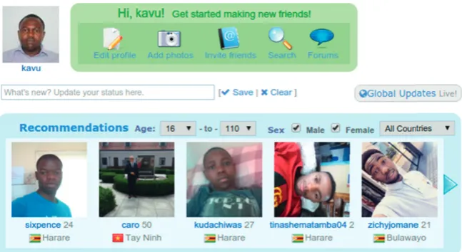
Figure 4 shows one of the author’s home pages just after logging in. A user received recommendations even before having friends on the platform since recommendations were derived from the user’s proﬁle. This approach eliminates the cold start problem which is also a serious problem in many RSs. When the logged in user clicks one of the recommended friends, the algorithm again com-putes new novel recommendations. User interactions were captured and exported as csv dataset for analysis, and

python libraries were used for analysis and for visuali-zation. The Jupyter notebook file where result analysis was performed is found on GitHub. From the data gathered for analysis, (TheUser) is the one that received recommen-dations and clicked (the user which was clicked by the TheUser). From the dataset, more than a thousand ommendations where generated and the first 700 rec-ommendations generated a lot of responses from the users. One thousand (1000) recommendations were offered to 250 users, which entailed that there were 250 active users on the platform and those 250 active users received rec-ommendations at least once from the algorithm.

Figure 5 shows the record of the number of active users and the time periods which they responded to recom-mendations. Redundant records were found in the form of one active user responding to more than one recommen-dation. The graph demonstrates that there was much activity in the morning as compared to other time sessions.

Considering the fact that, in Figure 6, the time sessions were encoded as follows: 0.0–1.0 (midnight), 1.0–2.0 (af-ternoon), 2.0–3.0 (evening), and 3.0–4.0 (morning), we can see that a lot of activity happens in the morning, probably, that is, when the users which were mostly students got free to chat on the platform. Figure 6 also shows that the ﬁrst 100 subject users responded a lot to their recommendations. This demonstrates that the algorithm was not aﬀected by the cold

Figure4: A snippet of recommendations made when a user logs in.

Morning Afternoon Evening

Night

Recommended session

Subject user

450

400

350

300

250

200

150

100

50

Figure 5: The relationship between subject users and recom-mendation time.

250

200

150

100 50 0

C

lic

k

ed us

er

Subjec

t user

250 200 150 100 50 0 0.0 0.5

1.0 1.5 2.0

2.5 3.0 3.5 _4.0

Clicked time

[image:11.600.139.463.72.249.2] [image:11.600.61.285.284.428.2] [image:11.600.313.545.291.408.2]

(12)

start problem. Cold start is failure to draw any inferences for new users due to insuﬃcient information of those users. The user proﬁles which participated in this experiment were not availed for analysis due to privacy issues from the service providers of the platform.

6. Discussion

Table 4 shows the first 20 records of user transactions. TheUser column is a unique identification of active users which received recommendations. The column Clicked represents the users which were clicked by TheUser, and ID numbers for TheUser is different from those for Clicked. If we look at The User1, we can see that the user is quite active, The User1 clicked ClickedID (5, 6, 11, and 3) at different times, that is, 11 : 42, 17 : 13, and 14 : 08, respectively. These users were clicked at different dates and time, showing that the algorithm was a bit dynamic and changes its recom-mendations with time and the user preferred those recommendations.

True positive (tp): refers to the recommended users which TheUser clicks.

False positive (fp): refers to the recommended users which TheUser did not click.

6.1. Precision. Since users where logged in sessions, it is important to ﬁgure out that unique recommendations per session can give us valuable information. Suppose that each session would take 10 minutes before a user is logged out, the total number of recommendations generated by the algo-rithms per the recorded transactions was 646. From these 646, those which the active users responded to were 77 per each unique session.

Therefore, the accuracy rate or precision is given below:

(tp/tp + fp)∗100.

6.2. Diversity. Diversity refers to the uniqueness of the recommended items, i.e., out of the recommended users how many were unique? Getting back to the recorded transactions, from the generated unique sessional mendations which were 646, 251 were unique recom-mendations (users which were never been recommended

before). This meant that the diversity rate of the algorithm

was (251/646)∗100�38.9% and shows that many of the

registered users where not active on the platform. There-fore, the algorithm was left with no option but to rec-ommend the remaining active users which were not that unique.

6.3. Coverage. Coverage looks at the total number of items on the platform, and out of the total, it identiﬁes how many of these were ever recommended during recommendations. From the time when the transactions were recorded, the social network had 1486 users, and out of these, 1115 were picked for recommendations. Therefore, coverage rate

be-comes users involved/total users�(1115/1486)∗100�75.03%.

6.4. Novelty. Novelty determines how unknown recom-mended items are to a user. The novelty of a retrieval set has been deﬁned with respect to the end user as the proportion of known and unknown relevant items in the recommended list [40].

That is, givenL⊆I_R, whereIRis the recommended list,Lis

the set of items inI_Rthat the user(u) likes,Lcan be partitioned

asL�L_k∪L_uinto those items,L_kis already known items to

the user, and L_u is unknown items to the user. Then, the

novelty per user is Novelty(R)�|Lu|/|L|, whereRis the set of all

active users who received recommendations. The average novelty of the algorithm is

􏽘 u∈R

L_u

􏼌􏼌􏼌 􏼌 􏼌􏼌􏼌􏼌/|L|

|R| �85.561%. (4)

This shows that the novelty of the algorithm was quite high, from the transactions which were recorded.

6.5. Serendipity. An item is serendipitous if it is novel and relevant [8]. Serendipity is the measure of how surprising the relevant recommendations are.

(1) Average number of recommendations:Rat time t₁

and timet₂

(2) Average number of obvious items on timet₁andt₂:q

(3) Number of nonobvious items on time t₁ and

t₂�R− q Table4: A snippet of recorded transactions.

[image:12.600.51.550.85.218.2]

(13)

S_user i:

count�0.0

∀iin[R− q]

if[R− q]are useful att₁andt₂

count�count+1

S_user

i�count/|totalRecommendations|

AverageSerendipity�􏽘

n_i _S

useri

totalrecommendations

􏼌􏼌􏼌

􏼌 􏼌􏼌􏼌􏼌

􏼠 􏼡�85.47%.

(5)

The best way to measure novelty and serendipity is asking users whether they were already familiar to a rec-ommended item. However, this is impracticable in oﬄine experiments [40]. It is for this reason that we took an online experimental approach to dealing with real users. The user’s familiarity with an item was tracked from the user’s history. If a user has been recommended an item before, that item is labeled familiar and is done implicitly. However, we did not consider other ways which the user might be familiar with the item.

Taking into consideration the level of novelty, seren-dipity, and dynamism of this algorithm, we can tell that the algorithm was really novel and serendipitous given that the rate was 84% at average. The level of novelty was better as compared to other novel algorithms which are found in the literature such as [40, 41] which experience a maximum of 77%. The algorithm’s recommendations were also changing with time sessions especially the four time sessions (morning, afternoon, evening, and midnight), which means it was considering time context very well. We found out that its accuracy rate was very low at 36%. It was discovered that there was a trade-off between serendipity and accuracy rate [42]. The hypothesis that, if an algorithm takes a holistic stance of incorporating contextual user profile in the form of social, cultural, psychological, and economic profile, to-gether with user-actioned items, that algorithm can offer dynamic, novel, and serendipitous recommendations was proven.

6.6. Conclusion. From the algorithm evaluation and the discussion made, we found out that the algorithm was quite novel and serendipitous, given that the average novelty and serendipity to each user was an average of 85%. The diversity of the algorithm was a bit low with an average of 38% due to the number of active users on the platform since the algorithm only considers active users to generate neighbourhood. This diversity is comparable to one of the best novel algorithms which were implemented by Hurley and Zhang [41] which had a novelty range of 38–44% and Zanitti et al. [43] which ranges from 25–52%. The platform did not perform well on poor mobile net-works, and this resulted in users visiting the platform only when using public networks or WiFi. This reduced the number of active users and aﬀected the performance of the algorithm. However, the coverage rate of the algorithm

was at an average rate of 75%, and this entails that the number of available active users were mostly considered when constructing recommendations. Finally, the article demonstrated that if a recommender algorithm is given timely and detailed proﬁles of users, dynamic, novel, and serendipitous recommendations can be realized, and this will increase (1) traﬃc on a site, (2) click streams, (3) desired decisions, and (4) retention rates.

7. Summary

This article proposed a novel mechanism of generating rec-ommendations based on a holistic understanding of user context to tackle three issues: (1) adequate adaptation to dy-namic user preferences, (2) user-centric recommendations (user satisfaction), (3) adequate novel and serendipitous rec-ommendations. The mechanism was further demonstrated as a process of deriving a user-centric recommender algorithm. The algorithm takes a hybrid approach of collecting holistic user contextual information which can be accessed from social media and then uses a user-user collaborative approach to generate and recognize novel, serendipitous, and dynamic recommendations. The holistic users’ contextual knowledge mainly involves the social, cultural, economic status, and psychological proﬁle of a user. The algorithm had an average

time complexity of O(n2_).

The results were quite promising for a social platform and we could not verify the performance of the algorithm over many platforms due to the lack of availability of other platforms to integrate with such as e-commerce and e-learning. This can be performed as future work. Another open issue is finding out which profile category among the four (social, cultural, psy-chological, and economic status) is more significant on plat-forms such as social networks, e-commerce, e-learning, movie sites, and online news. The social network did not allow users to tag most of their activities, and this also provided a limitation to this algorithm since the algorithm was supposed to be fed with updated user activities. Updated user activities would provide the algorithm with current interests and mood of users. In future, user activities could be tapped outside the service provider so that the algorithm is given a wider experience of a user to provide diverse and novel recommendations to the user. Our future work also involves developing an API that im-plements this algorithm so that different services can use the API to generate recommendations on different platforms.

Data Availability

The data used to support the ﬁndings of this study are available from the corresponding author upon request.

Conflicts of Interest

The authors declare that they have no conﬂicts of interest.

References

(14)

systems,” Expert Systems with Applications, vol. 42, no. 3, pp. 1743–1758, 2015.

[2] J. Beel, C. Breitinger, S. Langer, A. Lommatzsch, and B. Gipp, “Towards reproducibility in recommender-systems research,” User Modeling and User-Adapted Interaction, vol. 26, no. 1, pp. 69–101, 2016.

[3] F. O. Isinkaye, Y. O. Folajimi, and B. A. Ojokoh, “Recom-mendation systems: principles, methods and evaluation,” Egyptian Informatics Journal, vol. 16, no. 3, pp. 261–273, 2015. [4] P. Brusilovsky, A. Felfernig, P. Lops et al., “RecSys’16 Joint Workshop on Interfaces and Human Decision Making for Recommender Systems,” in Proceedings of the 10th ACM Conference on Recommender Systems, pp. 413-414, Boston, MA, USA, September 2016, https://dl.acm.org/citation.cfm? id�2959199.

[5] M. H. Aghdam, “Context-aware recommender systems using hierarchical hidden Markov model,” Physica A: Statistical Mechanics and Its Applications, vol. 518, pp. 89–98, 2019. [6] K. Haruna, M. A. Ismail, D. Damiasih, H. Chiroma, and

T. Herawan, “A comprehensive survey on comparisons across contextual pre-ﬁltering, contextual post-ﬁltering and con-textual modelling approaches,” Telkomnika (Telecommuni-cation Computing Electronics and Control), vol. 15, no. 4, pp. 1865–1874, 2017.

[7] D. Kotkov, S. Wang, and J. Veijalainen, “A survey of ser-endipity in recommender systems,” Knowledge-Based Sys-tems, vol. 111, pp. 180–192, 2016.

[8] S. Vargas, “Novelty and diversity evaluation and enhancement in recommender systems,” Ph.D. Dissertation, Universidad Aut´onoma de Madrid, Madrid, Spain, 2015.

[9] K. Lee and K. Lee, “Escaping your comfort zone: a graph-based recommender system for ﬁnding novel recommenda-tions among relevant items,”Expert Systems With Applica-tions, vol. 42, no. 10, pp. 4851–4858, 2015.

[10] T. D. Kavu, K. Dube, P. G. Raeth, and G. T. Hapanyengwi, “A characterisation and framework for user-centric factors in evaluation methods for recommender systems,”International Journal of ICT Research in Africa and the Middle East, vol. 6, no. 1, pp. 1–16, 2017.

[11] K. Verbert, N. Manouselis, X. Ochoa et al., “Context-aware recommender systems for learning: a survey and future challenges,” IEEE Transactions on Learning Technologies, vol. 5, no. 4, pp. 318–335, 2012.

[12] F. Ricci, L. Rokach, B. Shapira, and P. B. Kantor, Recom-mender Systems Handbook, Springer, Berlin, Germany, 2011. [13] M. G. Campana and F. Delmastro, “Recommender systems for online and mobile social networks: a survey,”Online Social Networks and Media, vol. 3-4, pp. 75–97, 2017.

[14] F. Keikha, M. Fathian, and M. R. Gholamian, “TB-CA: a hybrid method based on trust and context-aware for rec-ommender system in social networks,”Management Science Letters, vol. 5, no. 5, pp. 471–480, 2015.

[15] Li. Lei, “Next generation of recommender systems: algorithms and applications,” Dissertation, Digital Commons, Berkeley, CA, USA, 2014.

[16] M. Quadrana, P. Cremonesi, and D. Jannach, “Sequence-aware recommender systems,” ACM Computing Surveys, vol. 51, no. 4, pp. 1–36, 2018.

[17] L. Buchanan, Leigh Buchanan (2006), A Brief History of Decision Making, Harvard Business Publishing, Brighton, MA, USA, 2006.

[18] R. Chen, Q. Hua, Y.-S. Chang, B. Wang, L. Zhang, and X. Kong, “A survey of collaborative ﬁltering-based recom-mender systems: from traditional methods to hybrid methods

based on social networks,”IEEE Access, vol. 6, pp. 64301– 64320, 2018.

[19] M. Eirinaki, J. Gao, I. Varlamis, and K. Tserpes, “Recom-mender systems for large-scale social networks: a review of challenges and solutions,”Future Generation Computer Sys-tems, vol. 78, pp. 413–418, 2018.

[20] S. Karimi,A purchase decision-making process model of online consumers and its inﬂuential factor a cross sector analysis, Ph.D. thesis, pp. 1–326, 2013, https://www.escholar. manchester.ac.uk/api/datastream?publicationPid� uk-ac-man-scw:189583{&}datastreamId�FULL-TEXT.PDF.

[21] E. Frolov and I. Oseledets, “Tensor methods and recom-mender systems,” Wiley Interdisciplinary Reviews: Data Mining and Knowledge Discovery, vol. 7, no. 3, article e1201, 2017.

[22] C. C. Aggarwal, Recommender Systems, Springer, Berlin, Germany, 2016.

[23] Y. Koren, “Collaborative ﬁltering with temporal dynamics,” in Proceedings of the 15th ACM SIGKDD International Con-ference on Knowledge Discovery and Data Mining, Paris, France, June 2009.

[24] K. Kapoor, V. Kumar, L. Terveen, J. A. Konstan, and S. Paul, “I like to explore sometimes: adapting to dynamic user novelty preferences,” inProceedings of the 9th ACM Conference on Recommender Systems - RecSys’15, pp. 19–26, Vienna, Austria, September 2015.

[25] R. Mu, X. Zeng, and L. Han, “A survey of recommender systems based on deep learning,” IEEE Access, vol. 6, pp. 69009–69022, 2018.

[26] M. Taghavi, J. Bentahar, K. Bakhtiyari, and C. Hanachi, “New insights towards developing recommender systems,” The Computer Journal, vol. 61, no. 3, pp. 319–348, 2018. [27] C. V. Sundermann, M. A. Domingues, M. D. Silva Conrado,

and S. Oliveira Rezende, “Privileged contextual information for context-aware recommender systems,” Expert Systems with Applications, vol. 57, pp. 139–158, 2016.

[28] X. Yang, Y. Guo, Y. Liu, and H. Steck, “A survey of collab-orative ﬁltering based social recommender systems,” Com-puter Communications, vol. 41, pp. 1–10, 2014.

[29] Z. Yang, B. Wu, K. Zheng, X. Wang, and L. Lei, “A survey of collaborative ﬁltering-based recommender systems for mobile internet applications,” IEEE Access, vol. 4, pp. 3273–3287, 2016.

[30] B. P. Knijnenburg, M. C. Willemsen, Z. Gantner, H. Soncu, and C. Newell, “Explaining the user experience of recom-mender systems,” User Modeling and User-Adapted In-teraction, vol. 22, no. 4-5, pp. 441–504, 2012.

[31] J. J. Levandoski, M. Sarwat, E. Ahmed, and M. F. Mokbel, “LARS: a location-aware recommender system,”IEEE 28th International Conference on Data Engineering, vol. 1, pp. 450–461, 2012.

[32] S. Mahapatra and A. Tareen, “A cold start recommendation system using item correlation and user similarity,” ACM Transactions on Information Systems, 2015, https://www.acsu. buﬀalo.edu/{∼}suchismi/iRec.pdf.

[33] M. Millan, M. Trujillo, and E. Ortiz, “A collaborative rec-ommender system based on asymmetric user similarity,” in Proceedings of the 8th International Conference on Intelligent Data Engineering and Automated Learning (IDEAL’07), pp. 663–672, Springer-Verlag, Birmingham, UK, December 2007.

(15)

no. 4, pp. 1–6, 2014, http://www.ijcstjournal.org/volume-2/ issue-4/IJCST-V2I4P1.pdf.

[35] J. Leskovec,Mining of Massive Data Sets - Ullman, Cambridge University Press, Cambridge, UK, 2014.

[36] R. Singh, B. Kr. Patra, and B. Adhikari, “A complex network approach for collaborative recommendation,” CoRR, 2015, http://arxiv.org/abs/1510.00585.

[37] S. D. Sondur, S. Nayak, and A. P. Chigadani, “Similarity measures for recommender systems: a comparative study,” International Journal for Scientiﬁc Research and Development, vol. 2, no. 3, pp. 76–80, 2016, http://www.journal4research. org/Article.php?manuscript�J4RV2I3036.

[38] A. Said, A. Bellog´ın, A. De Vries, and B. Kille, “Information retrieval and user-centric recommender system evaluation,” inProceedings of the 21st Conference on User Modeling, Ad-aptation and Personalization (UMAP 2013), pp. 5–8, Rome, Italy, June 2013.

[39] C. Hayes, P. Massa, P. Avesani, and P. Cunningham, “An on-line evaluation framework for recommender systems,” in Proceedings of the Recommendation and Personalization in eCommerce (2002), p. 50, Malaga, Spain, January 2002. [40] L. Zhang, “The deﬁnition of novelty in recommendation

system,”Journal of Engineering Science and Technology Re-view, vol. 6, no. 3, pp. 141–145, 2013.

(16)

Hindawi

www.hindawi.com Volume 2018

Mathematics

Journal of

Hindawi

www.hindawi.com Volume 2018 Mathematical Problems in Engineering

Applied Mathematics

Hindawi

Probability and Statistics Hindawi

Hindawi

www.hindawi.com Volume 2018 Mathematical PhysicsAdvances in

Complex Analysis

Journal of

Hindawi

Optimization

Journal of Hindawi

Hindawi

Engineering Mathematics

International Journal of Hindawi

www.hindawi.com Volume 2018 Operations Research

Journal of

Hindawi

Function Spaces

Abstract and Applied Analysis Hindawi

www.hindawi.com Volume 2018 International

Journal of Mathematics and Mathematical Sciences

Hindawi

Hindawi Publishing Corporation

http://www.hindawi.com Volume 2013

Hindawi www.hindawi.com

World Journal

Volume 2018

Hindawi

www.hindawi.com Volume 2018Volume 2018

Numerical Analysis

Advances inAdvances in Discrete Dynamics in Nature and Society

Hindawi

www.hindawi.com Volume 2018 Hindawi

www.hindawi.com

Differential Equations

International Journal of

Volume 2018

Hindawi

Decision Sciences

Hindawi

Analysis

Hindawi

Stochastic Analysis

Submit your manuscripts at

(17)

MASSEY RESEARCH ONLINE

http://mro.massey.ac.nz/

Massey Documents by Type Journal Articles

Holistic User Context Aware Recommender Algorithm

Research Article