A spectrum matching method for accurate frequency estimation of real sinusoids

White Rose Research Online URL for this paper:

http://eprints.whiterose.ac.uk/145115/

Version: Accepted Version

Article:

Kui, W, McLernon, D orcid.org/0000-0002-5163-1975, Tu, Y et al. (2 more authors) (2019)

A spectrum matching method for accurate frequency estimation of real sinusoids. Review

of Scientific Instruments, 90 (4). 045112. ISSN 0034-6748

https://doi.org/10.1063/1.5091024

This article is protected by copyright. The following article has been accepted by Review of

Scientific Instruments. After it is published, it will be found at

https://aip.scitation.org/journal/rsi

[email protected] https://eprints.whiterose.ac.uk/

Reuse

Items deposited in White Rose Research Online are protected by copyright, with all rights reserved unless indicated otherwise. They may be downloaded and/or printed for private study, or other acts as permitted by national copyright laws. The publisher or other rights holders may allow further reproduction and re-use of the full text version. This is indicated by the licence information on the White Rose Research Online record for the item.

Takedown

If you consider content in White Rose Research Online to be in breach of UK law, please notify us by

A Spectrum Matching Method for Accurate Frequency

1

Estimation of Real Sinusoids

2

Kui Wang

1

, Yaqing Tu

1,*

, Des McLernon

2

, Yanlin Shen

3

and Peng Chen

1 3

1. Army Logistics University of PLA, Chongqing 401311, China. 4

2. The University of Leeds, LEEDS LS2 9JT, UK. 5

3. Logistics University of PAP, Tianjin 300309, China. 6

* Corresponding author. 7

Email: [email protected]; [email protected] 8

9 10

Abstract: It is well-known that incoherent sampling is detrimental for frequency estimation of a real 11

sinusoid, and the estimation errors get worse when the signal lengths are very short. In this paper, a spectrum 12

matching based frequency estimator is proposed as well as evaluated against other four two-step methods 13

developed to suppress the effect of incoherent sampling. The spectral interference introduced by incoherent 14

sampling is eliminated via a spectrum matching process including modulation and spectral analysis. A 15

further error correction based on Fourier transform is conducted to generate the fine frequency estimate. 16

Simulation results are carried out to show that the proposed method can closely approach the Cramér-Rao 17

lower bound without any error floor, and it can outperform the other four methods particularly for short 18

signal lengths. 19

Keywords: Frequency Estimation, Incoherent Sampling, Real Sinusoids, Spectrum Matching 20

21

I. INTRODUCTION 22

Frequency estimation of sinusoids has been a subject of investigation in many fields for decades, such as 23

radar, power systems, measurement and instrumentation. Numerous estimation approaches have been 24

developed so far. Given a straightforward operation of maximizing the periodogram [1], frequency domain 25

approaches based on the discrete Fourier transform (DFT) and implemented by the fast Fourier transform 26

(FFT) show high computational efficiency. A typical two-step scheme is widely concerned which usually 27

includes a coarse estimation via DFT to locate the spectral maximum, followed by a fractional interpolation 28

complex signals, and for real sinusoids, the inherent picket fence effect and spectral leakage of the DFT may 30

introduce significant errors if the signal is not coherently sampled [5, 6]. In addition, the DFT based methods 31

suffer from resolution loss when the signal lengths are very short. 32

In time domain, the two-step procedure is also introduced to promote the estimation performance. The 33

two-stage autocorrelation (TSA) approach [7] employs the linear property (LP) to reform the signal and 34

makes use of different lags of autocorrelations to produce frequency estimates. To avoid multiple 35

autocorrelations which are computationally burdensome, the Taylor expansion and the least squares (LS) 36

principle are involved to generate an error function in the extended autocorrelation (EA) method [8]. By 37

minimizing the error function, the performance of the EA method can approach the Cramér-Rao lower bound 38

(CRLB) when the signal lengths are sufficiently large. However, coping with incoherently sampled data in 39

short length, the EA method performs biased significantly because the signal autocorrelation has an error 40

term which is not negligible. Accordingly, the recently proposed phase match based (PM) method [9] and 41

phase correction autocorrelation (PCA) method [10] show different ways of reconstructing the 42

autocorrelation function to avoid the error term, and besides, the Cauchy inequality is also considered to 43

derive the error function in [9]. Generally, the PM and PCA methods are effective to deal with the 44

incoherently sampled signal, but their performance still shows slight degradation when the signal lengths are 45

very short. 46

In this paper, a new two-step frequency estimator based on spectrum matching is proposed, which shows 47

improvements in accuracy among the aforementioned two-step methods. The estimation bias caused by 48

incoherent sampling is effectively reduced by modulation, which has already been validated in our previous 49

work [11]. Then, spectral analysis is carried out to divide the original signal spectrum into two separated 50

complex versions, what we called spectrum matching. Finally, the fine estimate results from an error 51

correction via a classical approach based on Fourier transform [12]. The rest of the paper is organized as 52

follows: In Section II, the underlying principle to deal with the spectral interference caused by incoherent 53

sampling is interpreted. The whole algorithm is carried out in Section III. Performance comparison is 54

II. UNDERLYING PRINCIPLE 56

Consider a general, real sinusoid in noise as follows: 57

0

( ) cos( ) ( ), 1, 2,3,..., 1

x n A n w n n N (1) 58

where A and  represent the signal amplitude and the initial phase respectively; ₀(0₀) is the 59

angular frequency in radians; and w n( ) is the zero-mean additive white Gaussian noise (AWGN) with a 60

variance of 2_.

61

From [9, 10], we know that if the signal is incoherently sampled, the signal autocorrelation has an error 62

term which is only negligible for sufficiently large N. In frequency domain, the spectrum of the incoherently 63

sampled signal suffers from interference from the negative frequency components, and it gets worse for small 64

value of N. In addition, although the number of samples is increasing, the chosen value of ₀ can hardly

65

matches a frequency bin of the DFT, and so, it is inevitable to deal with the effect of incoherent sampling for

66

accurate frequency estimation. Now, with a priori knowledge of the signal frequency, which is provided by 67

the coarse estimation, the signal frequency can be directly modulated to approach coherent sampling. 68

Modulate the signal as ( ) ( ) jcn

m

x n x n e , and then 69

( 0 )  ( 0 ) 

( ) ( / 2) j cn ( / 2) j cn ( ) jcn

m

x n  A e     A e    w n e (2) 70

where _c (0c₀) is the modulation frequency.

71

Calculate the DFT of x nm( ), denoted as X km( ), as

72

( ) ( ) ( ) ( )

m m m m

X k S  k S  k W k (3)

73

where W km( ) is the DFT of the modulated noise; Sm( )k and Sm( )k are the DFT of the positive and

74

negative frequency exponentials in (2) respectively, which can be written as 75

















0 0 1

( ) ₀

2

0

1

( ) ₀

2

0

sin ( ) / 2

( )

2 sin ( ) / 2

sin ( ) / 2

( )

2 sin ( ) / 2

c k

c k

N

j _{c k}

j m

c k

N

j _{c k}

j m

c k

N A

S k e e

N A

S k e e

                     _{ }             _{ }      _  _{ }  (4) 76

where k2k N/ represents the k-th DFT frequency bin, and k0,1, 2,...,N1.

77

Note that in (4), we can force most values of Sm( )k or Sm( )k to be zero only by setting

0 c 2 m N/

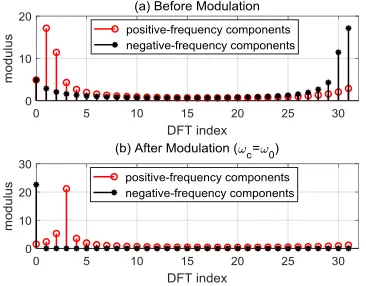
    or  ₀ c 2m N/ (m is an arbitrary integer). For example, in the absence of noise, if

79

we set _c ₀, the modulus of Sm( )k and Sm( )k are shown in Fig. 1 (00.0876 ,N32 and

80

/ 7

  ). Serious interference of the negative frequency components occurs in Fig. 1(a), and the frequency 81

estimation which ignores the negative frequency contribution will exhibit a significant bias. But in Fig. 1(b), 82

the negative frequency component has Sm( )k 0 for all values of k excluding k= 0, which means the

83

interference only exists at k= 0. Thus, if we can figure outS_m(0), it is possible to matchX k_m( ), which is the 84

spectrum of a real signal, to the spectrum of a complex sinusoid asSm( )k . The spectral interference of the

85

negative frequency components can be eliminated in this case. 86

[image:5.612.211.394.284.427.2]

87

Fig. 1. Interaction of positive and negative frequency components (zero noise). 88

89

III. METHOD DEVELOPMENT 90

A. Coarse Estimation 91

In practice, ₀ is unknown, and _c can only be set according to a coarse frequency estimate ˆ₀c. Assume 92

0 0 0

ˆc c

c











 



, where _₀c _{is the estimation error. Then, from (4) for}

0,1, 2,..., 1

k N , we get 93

0

1

( )

0 2

0

sin( / 2)

( ) ( 1) .

2 sin(( ) / 2)

c k

N c

j

k j

m c

k

N A

S k e e   

 



 

 

  

  (5) 94

Obviously, S_m( )k is proportional to sin(_N₀c/ 2)_{, and}

( ) 0

m

S_ k  when k0. Thus, we need 95

0

|_Nc| _{to be sufficiently small (empirically}

0

|_Nc| 0.1_{ ) so that the interference occurred at}

0 k can 96

estimate ˆ₀c _as 98 2 2 1 0 8 ˆ cos 4

c d d c

c

 _  _   _

 

  (6) 99

where

5 ( 2)[ ( ) ( 4)] K

k

d



_ r k r k r k , 1

4 ( 1)[ ( ) ( 2)]. K

k

c



_ r k r k r k The difference to [13] is that 100

we set

1

( ) N K ( )[ ( ) ( )]

n K

r k 



_{ } x n x n k x n k , k1, 2,3,...,K , and Kround(N/ 3), where round( )x

101

means to round x up or down to the nearest integer. This is to enhance the SNR according to the LP, and the 102

value of K is determined through simulations. Unlike the widely used FFT, the adopted coarse estimator does 103

not suffer from resolution loss for short signal lengths. 104

B. Spectrum Matching 105

Since most of the values of Sm( )k are forced to approximate zero after modulation, then the key problem

106

is to deal with the interference for k0. From (4), we know that 107









0

1

( ) ₀

2

0

sin ( ) / 2

(0) .

2 sin ( ) / 2

c N j _c j m c N A

S e e    

 

 _



 

 (7) 108

According to (3) and (4), for arbitrary value of integer q ( 0  q N 1), we can write 109









0

1

( ) 0

2

0

sin ( ) / 2

( ) ( ) ( ) ( ) .

2 sin ( ) / 2

c q

N

j c q

j

m m m m

c q

N A

S q X q S q W q e e      

  

 _{ }

 

 

   

  (8) 110

Then, substitute (8) for ( / 2)A ejin (7) and we obtain 111







 



1 0 2 0

sin ( ) / 2

(0) ( 1) ( ) ( ) ( ) .

sin ( ) / 2

q

N

j c q

q

m m m m

c

S e     X q S q W q

 



 

 

   

 (9)

112

Thus, substituting ˆ₀c for ₀ and _c in (9), we can define an estimator of Sm(0) as

113 1 0 2 0 ˆ

sin( / 2)

ˆ (0) ( 1) ( ).

ˆ sin( ) q c N j _q q

m c m

S e    X q









  (10) 114

Assuming that |₀c| is sufficiently small, it is easy to make the approximation to 115

0 0

0 0

ˆ

sin( / 2) sin(( ) / 2)

.

ˆ sin(( ) / 2)

sin( )

c

q c q

c c            

 (11) 116

ˆ _{(0) (0) ( ) ( )}

m m

S  S   q  q (12)

118

where ( )q and ( )q can be regarded as the terms of the estimation error caused by S_m( )q and the 119 modulated noise: 120









1 0 2 0

sin ( ) / 2

( ) ( 1) ( )

sin ( ) / 2

q

N

j c q

q

m c

q e     S q

        

 (13)

121









1 0 2 0

sin ( ) / 2

( ) ( 1) ( ).

sin ( ) / 2

q

N

j c q

q

m c

q e     W q



 

  

 

 (14)

122

Substitute (5) and



_c



ˆ₀c



₀ 



₀cinto (13), and as |_₀c| _{is assumed to be sufficiently small, so} 123





0 1 0 2 0

sin( / 2)

( ) cot( ) cot( / 2) .

2 c N c j j q A N

q  e e 

 _     _  ₍₁₅₎

124

Note that q can be an arbitrary integer from 1 to N-1, and we can set _q/ 2₀ to make ( )q 0. So 125

q can be approximated by setting _qround(_N ˆ₀c/ )_{. Furthermore, as we assumed that}

0 c_N



 is small in 126

(5), the value of ( )q can be sufficiently small to be ignored. 127

For ( )q , it is easy to prove thatE[ ( )] q 0, where E[ ] is the expectation operator. Then, from (12), we 128

can write 129

ˆ

E[Sm(0)]Sm(0)( ) E[ ( )]q   q Sm(0) (16)

130

which means that Sˆ_m(0) can be recognized as an unbiased estimator of S_m(0). 131

Now, we can divide the spectrum of the modulated real signal as X km( ) into two spectrums of complex

132

exponentials, as Sˆm( )k and Sˆm( )k , written as

133

ˆ ( ) ( ) ( (0) ˆ (0)) ( )

, 0,1, 2,..., 1 ˆ ( ) ( (0) ˆ (0)) ( )

m m m m

m m m

S k X k X S k

k N

S k X S k

           _{ }   

 (17)

134

where ( )k is the discrete Dirac Delta function with (0)1 and ( )k 0 for k0. Xm(0) can be

135

calculated by summing the elements of x nm( ). After this spectrum matching process, the signal amplitude

136

and initial phase can be directly estimated from Sˆ_m( )k as Aˆ2Sˆm(0) N and



ˆ angle S(ˆm(0)), but 137

here we focus on frequency estimation, which can be further derived from Sˆm( )k .

C. Error Correction 139

After modulation, the actual frequency of the positive frequency exponential in (2) has been shifted to 140

0 c

  . Accordingly, we can use 2ˆ₀c to approximately locate the spectral maximum of Sm( )k , which is

141

only ₀c _{radians distant from the actual value. Then, we could estimate} 0 c



 to correct the estimation bias 142

of ˆ₀c_{. According to the classical methodology of interpolation in frequency domain [12, 14], we can use two}

143

spectral points as S_m(2 ˆ₀c /N) andS_m(2 ˆ₀c /N) to realize accurate error correction. 144

From (4), we can calculate S_m(2 ˆ₀c /N), S_m(2 ˆ₀c /N), and after some simple algebra, we 145

obtain 146

0

1 1

0 0 2 2 0

0

ˆ

sin( ) cos( ) cos( ) sin( ) (2 ) cos( )

2 2 2 2 2 2

c

N N

c c c

j j

c N j

m

N A

S e e e

N N N

 _       _  _ _{ } _           

  (18)

147

0

1 1

0 0 2 2 0

0

ˆ

sin( ) cos( ) cos( ) sin( ) (2 ) cos( ).

2 2 2 2 2 2

c

N N

c c c

j j

c N j

m

N A

S e e e

N N N

 _       _  _{ } _           

  (19)

148

By subtracting the both sides of (18) and (19), making exp( (j N1) / N) 1 and tan( )x x for 149

sufficiently small x, after some simplification, we obtain 150

0 (2ˆ0 ) 0 (2ˆ0 )

c c c c

m m

S S

N N N N

   

 _   _ 

_{ }  _{  } _  _

   

    (20)

151

Substitute ˆ (2ˆ₀c / )

m

S _   N , ˆ (2ˆ₀c / )

m

S _   N for (2ˆ₀c / )

m

S _   N and (2ˆ₀c / )

m

S _   N , and take the 152

real part to avoid complex value. We can estimate ₀c as 153

0 0

0

0 0

ˆ _{(2ˆ / )} ˆ _{(2ˆ / )}

ˆ Re

ˆ _{(2ˆ / )} ˆ _{(2ˆ / )}

c c

c m m

c c

m m

S N S N

N S N S N

               _{  }          

  (21)

154

where ˆ (2ˆ₀c / )

m

S _   N can be calculated from the inverse DFT of Sˆm( )k in (17) as

155





0

1

ˆ

(2 / )

0

0

ˆ _{(2ˆc / )} N _{( ) (0)} ˆ _{(0) j} c _{N n.}

m m m m

n

S   N x n X S N e  



 

 



 

 



_   _ (22)

156

Finally, the fine frequency estimate (ˆ₀f_{) of our method can be calculated by}

0 0 0

ˆf ˆc ˆc

    . The overall 157

signal processing algorithm for the proposed method is shown in Table I. 158

TABLEI 160

SIGNAL PROCESSING ALGORITHM

161

1 Calculate the coarse frequency estimate ˆ0 c  via (6).

2 Modulate x n( ) with ˆ0 c c

  to obtain x nm( ) as in (2).

3 Calculate round( ˆ0/ ) c

q N  and 1

0

( ) N ( ) jqn

m n m

X q 



_x n e . 4 Calculate Sˆm(0) according to (10).

5 Calculate ˆ (2ˆ0 / ) c m

S   N and ˆ (2ˆ0 / ) c m

S   N via (22)

6 Generate the frequency correction factor ˆ0 c 

 via (21).

7 Obtain the fine frequency estimate byˆ0 ˆ0 ˆ0

f c c

    . 162

IV. SIMULATION RESULTS 163

To evaluate the performance of the aforementioned two-step methods, we use the TSA [7], EA [8], PM [9], 164

and PCA [10] methods as a comparison against our proposed method. Without loss of generality, we assume 165

1

A , and  is uniformly distributed between  and . Each simulation result is carried out with an 166

average of 2000 independent Monte Carlo runs. 167

Bounds As with the approximation made in [15], the CRLB of frequency estimation for a real sinusoid is 168

given as 169

0 2

12 ˆ

CRLB var[ ]

SNR ( 1)

f

N N



 

  (26) 170

where the SNR is defined as 2 2

/ (2 ) A  . 171

Variable Frequency: Because of the periodicity of the spectrum of a real sinusoid, we only evaluate the 172

performance for 0₀0.5 . The root-mean-square error (RMSE) versus signal frequency ₀ for 173

32

N for four different SNR values is presented in Fig. 2. The signal frequency varies from 0.01 to 174

0.49with a step size of 0.01 . The enlarged scale of 1.5  ₀3.5 can show the advantages of the 175

proposed method more clearly. When the signal frequency is very low, the PCA and EA methods provide 176

more reliable accuracy at SNR=10dB in Fig.2 (a), while the PM method performs better for high SNRs in Fig. 177

2 (c) and (d). However, generally speaking, the proposed method shows higher accuracy than the other 178

evaluated methods in a very large range of signal frequency, and the superiority becomes more obvious with 179

181

[image:10.612.97.496.79.310.2]

182

Fig. 2. RMSE versus 0 for N=32. (a) SNR=10dB; (b) SNR=30dB; (c) SNR=50dB; (d) SNR=70dB. 183

184

Variable SNR: The RMSE versus SNR for₀0.09and N32 is shown in Fig. 3. The SNR varies 185

from -10dB to 119dB with a step size of 3dB. The effect of RMSE saturation can be found for the EA and 186

PCA methods, which has proved their biasness in this case. By contrast, the TSA, PM and proposed methods 187

can follow the trend of the CRLB without error floors, but only the proposed method can asymptotically 188

approach the CRLB for sufficiently large SNRs. 189

190

Fig. 3. RMSE versus SNR for 00.09and N32. 191

192

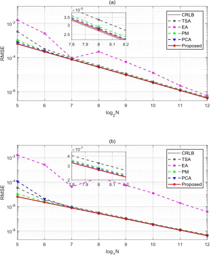
[image:10.612.213.393.491.634.2]

in Fig. 4. The reformed signal length log2N continuously increases from 5 to 12 (32 to 4096 for N). For two

194

SNR values of 30dB and 70dB, evident advantages of the proposed method can be found for short signal 195

lengths (eg. N<128). With increasing the signal length, all the TSA, PM, PCA and the proposed methods can 196

closely follow the CRLB. However, from the enlarged subgraph, we can see the proposed method is even 197

slightly better than the other evaluated methods. 198

199

[image:11.612.197.408.196.451.2]

200

Fig. 4. RMSE versus log2N for00.09. 201

(a) SNR=30dB; (b) SNR=70dB. 202

203

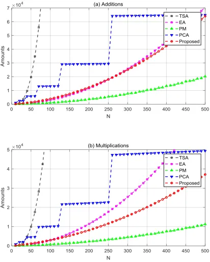
Computational Complexity: The result of the comparison of computational complexity is shown in Table 204

II. All the complex-valued (CV) operations are converted to real-valued (RV) additions and multiplications, 205

following the principle listed on the right-hand part of Table II. We neglect all the computations with O(1) 206

complexity. To make the comparison more clearly, the amount of required additions and multiplications for 207

the evaluated methods is shown in Fig. 5. The signal length N varies from 10 to 500 with a step size of 10. 208

Obviously, we can see the computational complexity of the proposed method is only higher than the PM 209

method, while the TSA, EA and PCA methods require more additions and multiplications within the 210

[image:12.612.85.520.90.187.2]

TABLE II 212

Comparison of Computational Complexity. 213

Method Addition Multiplication Converting Principle

Operation Addition Multiplication

TSA [7] 2NM02M028M03/ 3 32 N

2 2 3

0 0 4 0/ 3 26 0/ 3 16

NM M  M  M  N CV CV 2 4

EA [8] 5N2/ 18 5 N/ 2 2

5N / 18 3 N/ 2 CV RV 0 2

PM [9] 2Np4p28p 2

2 9

Np p  p CV+CV 2 0

PCA [10] 3 2M1 2M1 3

M   N 2 2

2M 2M 41 / 3

M     N CV+RV 1 0

Proposed 2

2N / 9 51 N/ 3 2

/ 9 56 / 3 N  N

Note: M0(N1) / 2,p0.46N,M log 22 N, where   x or   x means to round x down or up to the nearest integer.

214

215

[image:12.612.203.409.231.488.2]

216

Fig. 5. Amounts of additions and multiplications versus N. 217

(a) Additions; (b) Multiplications. 218

V. CONCLUSION 219

In this paper, a spectrum matching based method is proposed to realize frequency estimation of an 220

incoherently sampled real sinusoid. Compared with other four methods designed to solve this problem, the 221

proposed method shows better performance when the signal lengths are short. As long as the SNR reaches a 222

certain level, the proposed method can closely approach the CRLB without any error floor, which means, the 223

proposed method can be very useful in some high SNR applications such as measurement and 224

process can be also used for the estimation of signal amplitude and initial phase. 226

ACKNOWLEDGMENTS 227

The study is supported by National Natural Science Foundation of China (NNSFC) (61871402), 228

Postgraduate research innovation project of Chongqing (CYB14100), Natural Science Foundation of Tianjin 229

(18JCQNJC01400), Key Program of Natural Science Foundation of Chongqing (cstc2015 jcyjBX0017), PhD 230

startup foundation (WHB201707) and Special Project for 100 Academic and Discipline Talents of 231

Chongqing (2012-44). 232

233

REFERENCES 234

[1] D. C. Rife, R. R. Boorstyn, “Single tone parameter estimation from discrete-time observations”, IEEE

235

Trans. Inform. Theory. 20_{, 591-598 (1974).}

236

[2] E. Jacobsen, P. Kootsookos, “Fast, accurate frequency estimators”, IEEE Signal Process. Mag. 24_,

237

123-125, (2007).

238

[3] C. Candan, “A method for fine resolution frequency estimation from three DFT samples”, IEEE Signal

239

Process. Lett. 18_{, 351-354 (2011).}

240

[4] C. Candan, “Fine resolution frequency estimation from three DFT samples: Case of windowed data”,

241

Signal Process. 114 _{245-250 (2015).}

242

[5] Shanglin Ye, Jiadong Sun, and Elias Aboutanios, “On the Estimation of the Parameters of a Real

243

Sinusoid in Noise”, IEEE Signal Process. Lett. 24_{, 638-642 (2017).}

244

[6] Slobodan Djukanović, “An Accurate Method for Frequency Estimation of a Real Sinusoid”, IEEE

245

Signal Process. Lett. 23_{, 915-918 (2016).}

246

[7] Lui K W K, So H C, “Two-stage autocorrelation approach for accurate single sinusoidal frequency

247

estimation”, Signal Process. 8, 1852-1857 (2008).

248

[8] Y. Cao, G. Wei, and F.-J. Chen, “A closed-form expanded autocorrelation method for frequency

249

estimation of a sinusoid,” Signal Process. 92_{, 885}–_{892 (2012).}

250

[9] Yanlin Shen, Yaqing Tu, Linjun Chen and Tingao Shen, “A phase match based frequency estimation

251

method for sinusoidal signals”, Rev. Sci. Instrum. 86_{, 045101 (2015).}

252

[10]Yaqing Tu, Yanlin Shen, “Phase correction autocorrelation-based frequency estimation method for

253

sinusoidal signal”, Signal Process. 130_{, 183-189 (2016).}

[11]Kui Wang, Yaqing Tu, Yanlin Shen, Wei Xiao, “A modulation based phase difference estimator for real

255

sinusoids to compensate for incoherent sampling”, Rev. Sci. Instrum., 89_{, 085120 (2018).}

256

[12]E. Aboutanios, B. Mulgrew, “Iterative frequency estimation by interpolation on Fourier coefficients”,

257

IEEE Trans. Signal Process. 53_{, 1237-1242 (2005).}

258

[13]Kenneth Wing Kin Lui and Hing Cheung So, “Modified Pisarenko Harmonic Decomposition for

259

Single-Tone Frequency Estimation”, IEEE Trans. Signal Process.56_{, 3351-3356 (2008).}

260

[14]Lei Fan, Guoqing Qi,“Frequency estimator of sinusoid based on interpolation of three DFT spectral

261

lines”, Signal Process. 144_{, 52-60 (2017).}

262

[15]M. Kay Steven, “Fundamentals of Statistical Signal Processing, Volume I: Estimation theory”, Upper

263

Saddle River, NJ, USA: Prentice-Hall, (1993).