http://wrap.warwick.ac.uk/
Original citation:Ladroue, Christophe and Papavaviliou, Anastasia. (2013) A distributed procedure for computing stochastic expansions with mathematica. Journal of Statistical Software, Volume 53 (Numbe 11).
Permanent WRAP url:
http://wrap.warwick.ac.uk/57604
Copyright and reuse:
The Warwick Research Archive Portal (WRAP) makes this work of researchers of the University of Warwick available open access under the following conditions.
This article is made available under the Creative Commons Attribution- 3.0 Unported (CC BY 3.0) license and may be reused according to the conditions of the license. For more details seehttp://creativecommons.org/licenses/by/3.0/
A note on versions:
The version presented in WRAP is the published version, or, version of record, and may be cited as it appears here.
May 2013, Volume 53, Issue 11. http://www.jstatsoft.org/
A Distributed Procedure for Computing Stochastic
Expansions with
Mathematica
Christophe Ladroue University of Warwick
Anastasia Papavasiliou University of Warwick
Abstract
The solution of a (stochastic) differential equation can be locally approximated by a (stochastic) expansion. If the vector field of the differential equation is a polynomial, the corresponding expansion is a linear combination of iterated integrals of the drivers and can be calculated using Picard Iterations. However, such expansions grow exponentially fast in their number of terms, due to their specific algebra, rendering their practical use limited.
We present aMathematicaprocedure that addresses this issue by reparametrizing the polynomials and distributing the load in as small as possible parts that can be processed and manipulated independently, thus alleviating large memory requirements and being perfectly suited for parallelized computation. We also present an iterative implementation of the shuffle product (as opposed to a recursive one, more usually implemented) as well as a fast way for calculating the expectation of iterated Stratonovich integrals for Brownian motion.
Keywords: rough paths, stochastic expansion, iterated integral, picard iteration, simulation, Mathematica.
1. Motivation and mathematical background
1.1. Motivation and notation
Consider the following stochastic differential equation (SDE):
dYt=f(Yt, θ)dXt (1)
whereYt∈Rm,Xt∈Rn and f(., θ)∈Rm×n. The parameters of the function f are collected
in the variable θ. We call each X(i) a driver of the differential equation. We assume the functionsfj,i, i∈ {1. . . n}, j ∈ {1. . . m} to be polynomials. The initial value of Yt is set to Y0.
The objective is to derive a local approximation of the solution in terms of f, Y0 and the
iterated integrals ofYt, i.e., that is integrals of the form
Z
. . .
Z
0<u1<···<uk≤T
dXτ1 u1. . . dX
τk
uk
for any word τ = (τ1, . . . , τk) constituted of the letter τi ∈ {1, . . . , n}, i = 1, . . . , k.. Such expansions play an important role in the theory of rough paths, allowing one to define such a differential equation for a large class of driversX (Lyons and Qian 2003). They have also been used recently for parameter estimation of SDE (Papavasiliou and Ladroue 2010).
Iterated integrals have been implemented inMathematicabefore. Kendall(2005) showed how to manipulate stochastic integrals symbolically by implementing the rules of Itˆo calculus. Their package Itosvn3 could also compute analytic forms of the expectation of stochastic integrals. For example, once the user provided the solution of an SDE in terms of stochastic integrals, its moments could be calculated. In this paper’s setting however, the solution is not known and is analytically approximated with Stratonovitch calculus. Tocino (2009) pre-sented an implementation of iterated integral calculus that realized both Itˆo and Stratonovitch variants and used it to derive a number of new relations for iterated integrals products and powers. However, as the number of terms to consider grows exponentially with every product, this implementation will not scale up.
1.2. Picard iterations
Picard iterations provide a way for deriving local approximations of solutions of differential equation. They are defined as:
Y0,T(0) = Y0−Y0= 0 (2)
Y0,T(r+ 1, j) = n
X
i=1
Z
fj,i(Ys(r, j))dXs(i) (3)
(4)
whereY0,T(r, j) is thej-th component of the approximation ofY0,T =
RT
0 dYs=YT−Y0 after
r iterations. Thus, the first iteration gives:
Y0,T(1, j) =
Z t
0
fj,1(Y0)dXs(1)+. . .+
Z t
0
fj,n(Y0)dXs(n) (5)
Note that if we are interested in the actual value of the solution at a timet∈[0, T], its Picard approximation is given by
One of the main successes in the theory of rough paths was to give precise conditions onX andf for Picard iterations to converge (Lyons and Qian 2003).
1.3. Iterated integrals
Iterated integrals are integrals of the form:
Xs,t(τ)=
Z
. . .
Z
s<u1<...<uk<t
dX(τ1) u1 . . . dX
(τk)
uk
whereτ = (τ1, . . . , τk) is called a word, with lettersτi ∈ {1. . . n}, i= 1, . . . , k. By definition, integrating an iterated integral produces an iterated integral:
Z T
0
X0(τ,s)dXs(j) =
Z T
0
Z
. . .
Z
0<u1<...<uk<s
dX(τ1) u1 . . . dX
(τk)
uk dX
(j)
s (6)
= X(τ1,...,τk,j)
0,T (7)
If X is a geometric p-rough path, i.e., it can be approximated by paths of bounded varia-tion (see Lyons and Qian (2003) for a precise definition), then the integrals obey the usual integration-by-parts rule, which can be generalized as follows:
Xs,t(τ)Xs,t(ρ) = X α∈τtρ
Xs,t(α) (8)
The shuffle producttof two words τ andρis the set of all words using the letters inτ and ρ such that they are in their original order. For example 13t42 ={1342,1432,4132,1423,4213, 4132} but 1324, for example, does not belong to the set.
This result holds only in the case of deterministic drivers X, or Stratonovitch integrals. A similar relation exists for Itˆo integrals but requires a small correcting term (Tocino 2009) making them slightly less practical in this context. A simple transformation allows diffusion processes to be defined with respect to Itˆo or Stratonovitch integrals (Kloeden and Platen 1991):
dyt=µ(yt)dt+σ(yt)dBt⇔dyt=
µ(yt)− 1 2σ
0(y
t)σ(yt)
dt+σ(yt)◦dBt
It immediately follows from Equation 8 that any power of an iterated integral is a sum of iterated integrals and that a polynomial of iterated integrals is also a linear combination of single iterated integrals. For example:
X0(1),TX0(2,T,3) = X0(1,T,2,3)+X0(2,T,1,3)+X0(2,T,3,1)
X0(1),T2 = X0(1),TX0(1),T
= X0(1,T,1)+X0(1,T,1)
= 2X0(1,T,1)
X0(1),T` = `!X0(1,T,...,1)
X0(0,T,1,0)X0(1,T,1) = X0(0,T,1,0,1,1)+ 2X0(0,T,1,1,0,1)+ 3X0(0,T,1,1,1,0)
The number of terms from the product of iterated integrals grows fast, exponentially if all letters are different.
1.4. Expansions
We are now in position to derive expansions for the solution of a differential equation. Picard iterations yield:
Y0,T(0, j) = 0
Y0,T(1, j) =
Z
0,T
fj1(Ys(0))dXs(1)+. . .+
Z
0,T
fjn(Ys(0))dXs(n)
= fj1(Y0)X0(1),T +. . .+fjn(Y0)X0(n,T)
Y0,T(2, j) =
Z
0,T
fj1(Ys(1))dXs(1)+. . .+
Z
0,T
fjn(Ys(1))dXs(n)
=
Z
0,T
fj1(Y0,s(1) +Y0)dXs(1)+. . .+
Z
0,T
fjn(Ys(1) +Y0)dXs(n)
Since Y0,s(1, .) is a sum of iterated integrals, the polynomials fji(Ys(1) +Y0) are also sums
of iterated integrals and so is their integration with respect toX(i). Y0,T(2) is thus a sum of iterated integrals and by recursion allY0,T(r, .) are. A formal proof in the context of differential equations driven by rough paths can be found inPapavasiliou and Ladroue(2010).
Example
Consider the Ornstein-Uhlenbeck process: dyt=a(1−yt)dt+bdWt andy0 = 0. In this case,
Xt(1) =t,Xt(2)=Wt and Y0(i)= 0 for i∈ {1,2}. Applying Picard iterations, we obtain:
Y0,T(0) = 0
Y0,T(1) =
Z T
0
a(1−0)dXs(1)+
Z T
0
bdXs(2)
= aX0(1),T +bX0(2),T
Y0,T(2) =
Z T
0
a(1−(aXs(1)+bXs(2)))dXs(1)+
Z T
0
bdXs(2)
= aX0(1),T −a2X0(1,T,1)−abX0(2,T,1)+bX0(2),T
Y0,T(3) = aX0(1),T −a2X0(1,T,1)+a3X0(1,T,1,1)+abX0(2,T,1,1)+abX0(2,T,1)+bX0(2),T
The solution of the stochastic differential equation can thus be approximated by a series of iterated integral of the drivers, whose coefficients are a function of the parameters. The iterated integrals capture the statistics of the drivers and are separated from the parameters.
2. Reparametrization of the polynomials
One thing to note in the derivation of expansions is that each successive iterations requires the explicit linear combination of iterated integrals for the previous iteration; evaluatingY0,T(r) requires the complete expansion forY0,T(r−1). As the number of terms grows, manipulating this object rapidly becomes unwieldy.
In this section, we describe a reparametrization of the polynomials which bypasses the need for an expansion in terms of iterated integrals. It provides a more compact representation of the approximate solution and is naturally amenable to parallel processing. For clarity of exposition, we first introduce the approach in the case of a one-dimensional (m = 1) differential equation with n drivers. We assume the polynomials f1i to be of degree less or equal toq. In the last subsection, the procedure is generalized to m-dimensional differential equations.
2.1. One-dimensional case
We first remark that a polynomialP(y) can be written in terms ofy−y0 by writing its Taylor
expansion aroundy0:
P(y) = q
X
k=0
1 k!∂
kP(y
0)(y−y0)k (9)
Next we introduce the following new operation for iterated integrals:
Xs,tα BXs,tβ =
Z t
s
Xs,uα dXs,uβ =
Z t
s
Xs,uα Xβ−
s,udXuβend (10)
whereβ− is the word β with the last letter removed and βend the last letter of β. This is a
non-associative, non-commutative operation – in fact, it can be viewed as a non-commutative dendriform. We can rewrite the Picard iteration using this operation. Note that from now on, the interval [s, t] will be fixed to [0, T] and will be omitted.
Y(0) = y0−y0= 0 (11)
Y(1) = n
X
i=1
Z T
0
fj1(Ys(0) +y0)dXs(i) (12)
= n
X
i=1
fj1(y0)X(i) (13)
Y(r+ 1) = n
X
i=1
f1i(Ys(r) +y0)BX(i) (14)
= n X i=1 q X k=0 1 k!∂ kf
1i(y0)Ys(r)kBX(i) (15)
= q
X
k=0
((Ys(r))k B n
X
i=1
(∂kf1i(y0)X(i))
!
(16)
Therefore, if we define the objectsQas:
Qk= n X i=1 1 k!∂ kf
the Picard iteration takes the following form:
Y(1) = Q0
Y(r+ 1) = q
X
k=0
Y(r)k BQk
whereY(r)k is the usual product.
2.2. Description of the approach
Consider a one-dimensional differential equation with quadratic functionsf1i, i.e.,q = 2. The new representation yields:
Y(1) = Q0 (18)
Y(2) = 1BQ0+Q0 BQ1+ (Q0)2 BQ2 (19)
= Q0+Q0 BQ1+ (Q0)2 BQ2 (20)
Y(3) = Q0+ (Q0+Q0BQ1+ (Q0)2BQ2)BQ1 (21)
+(Q0+Q0BQ1+ (Q0)2 BQ2)2BQ2 (22)
where (Qk)` is thek-th object Q to the power`. Crucially, this new representation does not require the explicit computation of the shuffle products, keeping the number of terms under control. Moreover, the expression can be expanded into its summands and each summand be processed independently. Thus, we avoid the handling of a large expression and are able to parallelize the computation.
Note that the representation only depends on the maximum degree of the polynomials but not on the number of drivers. The Picard iteration can therefore be done only once, stored in a file and used at a later date for any system that uses the same maximum degreeq.
Using this representation, it is possible to derive the stochastic expansions through a few stages:
1. Expand the expressionY(r) into its monomialsu. Each monomialuis a function ofQ’s that uses the non-commutative products. Importantly, the objects Qand the product
B are only used as place-holders at that stage. For example, the first three monomials forY(3) areQ0,Q0 BQ1 and (Q0BQ1)BQ1.
2. For each monomial u, the objects Q are replaced by their values from the model at hand. Each Q is a weighted sum of the drivers X(i) (Equation17), so each u becomes
a polynomial V of X(i) in terms of the non-commutative product. As in the previous step, the product is still only employed as a place-holder and not instantiated.
3. Each polynomialV is expanded into its monomials v. Each v is a function ofX(i) and
B.
Each process only requires a fraction of the memory that a direct approach (replacingQ’s by theX(i) and using the product’s definition) would. Moreover, at all stages, each monomial can be processed independently from the rest, leading to natural parallelization. It is also important to note that the whole expression is actually stored in a file and thus not in memory at any point. The exact details of this procedure are given in Section 3.
2.3. Generalization
In the multidimensional case, the Taylor expansion of a polynomial requires a larger number of terms that involve cross-products between the components of the vector Y. The objectsQ are not indexed by k ∈ {0, . . . , q} but by the set OWm(0, q) of the ordered words of length up toq written with letters {1, . . . , m} and are now defined as:
Qτj = n
X
i=1
|τ|!
c(τ)∂τfji(Y0)X
(i) (23)
forj∈ {1, . . . , m}. The constantc(τ) is the number of different words we can construct using the letters in τ. The Picard iteration becomes:
Y(1)(j)=Q∅j andY(r+ 1)(j)= X τ∈OWm(0,q)
Y(r)τ BQτj
3. Implementation
This section describes how this new approach was implemented inMathematica. In this part, iterated integrals of the drivers (X(i1,...,in)) are denoted j(i1,...,in) to follow convention and
drivers are numbered from 0 with the first driver representing time.
3.1. Shuffle product
Since each product of two iterated integrals is a shuffle product, special care must be taken of its implementation. Tocino (2009) has shown a way of writing the product in Mathematica:
Tocino[j[{x_}], j[a_List]] :=
Sum[j[Insert[a, x, k]], {k, 1, Length@a + 1}]; Tocino[j[a_List], j[{x_}]] := Tocino[j[{x}], j[a]]; Tocino[j[a_List], j[b_List]] :=
Ap[Tocino[j[a], j[Drop[b, -1]]], Last@b] +
Ap[Tocino[j[Drop[a, -1]], j[b]], Last@a]
/; (Length@a > 1 && Length@b > 1);
This is a direct and natural translation of the following result:
JαJβ =
Z
Jα−JβdJαend+
Z
JαJβ−dJβend
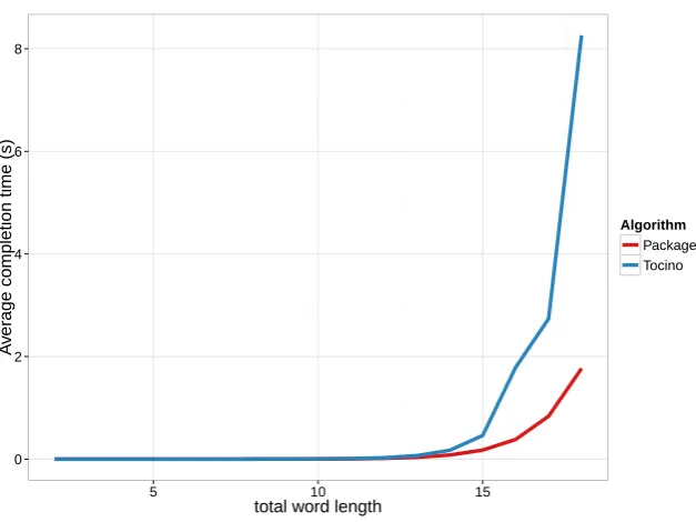
0 2 4 6 8
5 10 15
total word length
A
v
er
age completion time (s)
[image:9.595.141.455.108.343.2]Algorithm Package Tocino
Figure 1: Average time taken to compute a shuffle product, as a function of the words’ total length.
of two wordsα andβ, we first set the string ‘aa...aabb..bb’, with as manya’s andb’s as there are letters in α and β respectively (line 2). We then replace all occurrences of ‘ab’ by ‘ba’ (line 6) and keep on iterating the replacement until none are possible (i.e when the word is ‘bb..bbaa..aa’) while keeping track of the new words generated (lines 4–6). The set of all words thus created is the shuffle product of two arbitrary words of the same lengths ofα and β. Finally, the lettersa andb in each word are replaced by their actual values fromα and β (lines 7–9).
Shuffle[a_List,b_List]:=Module[{list,u,v},
u={StringJoin@Join[Table["a",{Length[a]}],Table["b",{Length[b]}]]}; v=Table[0,{StringLength[u[[1]]]}];
list=Flatten@NestWhileList[
DeleteDuplicates@Flatten@
StringReplaceList[#,"ab"->"ba"]&,u,#!={}&]; (v[[#[[1]]&/@StringPosition[#,"a"]]]=a;
v[[#[[1]]&/@StringPosition[#,"b"]]]=b; v)&/@list];
3.2. Non-commutative product
The non-commutative and non-associative product B is implemented as in Mathematica, an operation with no built-in meaning. We only set a few basic properties for this product:
Unprotect[CircleDot]; (* $\odot$ = esc c . esc *) 1$\odot$x_ := x;
x_$\odot$1 := 0; 0$\odot$x_ := 0; x_$\odot$0 := 0; Protect[CircleDot];
Sinceis only used as a placeholder, its actual definition in terms of shuffle product (Equa-tion10) is coded in another function, NCP:
NCP[0, j[b_List]] := 0; NCP[1, j[b_List]] := j[b]; NCP[j[a_List], 0] := 0; NCP[j[a_List], 1] := j[a]; NCP[j[a_List], j[{}]] := j[a]; NCP[j[a_List], j[b_List]] :=
Ap[j[a]*j[Drop[b, -1]], Last[b]] /; Length[b] > 0; NCP[n_*j[a_List], j[b_List]] := n*NCP[j[a], j[b]];
NCP[j[a_List], n_*j[b_List]] := n*NCP[j[a], j[b]]; NCP[n_*j[a_List], m_*j[b_List]] := n*m*NCP[j[a], j[b]]; NCP[x_ + y_, z_] := NCP[x, z] + NCP[y, z];
NCP[x_, y_ + z_] := NCP[x, y] + NCP[x, z];
NCP[x_*(y_ + z_), t_] := NCP[x*y, t] + NCP[x*z, t]; NCP[(y_ + z_)*x_, t_] := NCP[x*y, t] + NCP[x*z, t];
3.3. Picard iteration
The usual Picard iteration is implemented with a helper function PicardIteration as fol-lowing:
PicardIteration[f_List,X_]:=
Total[MapIndexed[(Ap[#1[X]*j[{}],First[#2]-1])&,f]] Picard[f_List,X0_,n_Integer]:=
Nest[(PicardIteration[f,#])&,X0,n]
For example, Picard[f,x0,4] outputs the stochastic approximation of the SDE with the functions f collected in a list in the first argument. This was used in Papavasiliou and Ladroue (2010) for a system with linear drift and quadratic variance.
With the new representation in Q, it can be written directly as in Equation2:
PicardQ1Dim[Q_, R_, q_] :=
Ris the number of iterations to be calculated and qthe maximum degree of the polynomials f. PicardQ1Dim[] produces a very compact representation of the expansion, which needs to be processed further in order to give the same result asPicard[].
3.4. Expectation of an iterated integral
It is often of interest to calculate the moments of the solution of the SDE and this can be approximated by computing the moments of the stochastic expansion. Since the expansion is a weighted sum of iterated integrals j, its expectation is simply the weighted sum of the integrals’ expectations. If the drivers consist of time and Brownian motions, the expectation of an iterated integral has a simple analytic form that can be arrived at recursively (Tocino 2009).
Here we present a more direct way of calculating this quantity. Given a wordαand assuming Wiener processes (Ladroue 2010):
EJα(t) =
0 ifα is not a sequence of 0 and pairsmm pαt
qα
qα! otherwise
wherepα= 12 #{αi6=0}
2 andq
α= 12(#{αi = 06 }) + (#{αi = 0}). Thus, for example: EJ(0,1,1,0,0) = 1/22/2t(3+2/2)/(3 + 2/2)! = 48t4
EJ(0,1,1,0,0,1) = 0
EJ(2,2,1,1,3,3) = 1/26/2t(0+6/2)/(0 + 6/2)! = 48t3 EJ(2,2,0,1,1,3,3,0,0,0) = 1/26/2t(4+6/2)/(4 + 6/2)! = t7
8.7!
This result is implemented in Mathematica. The expectation for a word α is then calculated in at most |α|steps:
ExpSBM[t_, j[a_List]] := Module[{i, c}, i = Length@a;
c = {0, 0}; Catch[
While[i > 0, If[a[[i]] == 0,
c += {0, 1}; i--,
If[(i > 1) && (a[[i]] == a[[i - 1]]), c += {1, 1}; i -= 2,
c = {Infinity, 0}; Throw@0 ]]]];
(1/2)^First@c t^Last@c/(Last@c)!];
3.5. Distributed processing of monomials
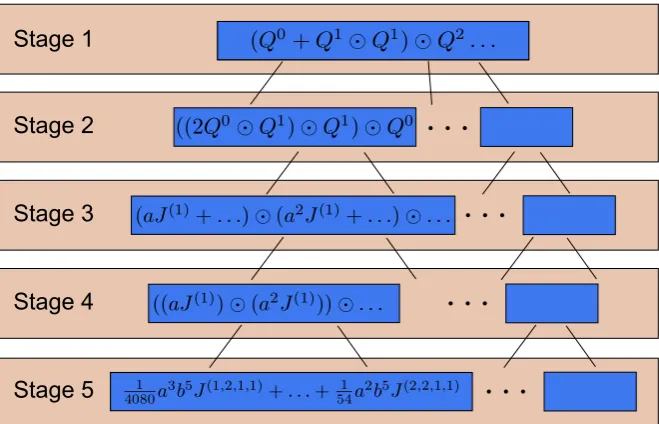
Going from the compact representation provided byPicardQ1Dim[]to the linear combination of iterated integralsj’s is done in a few stages. Each stage modifies the representation of the stochastic expansion in such a way that a) computational requirements are minimized and b) it can be parallelized.
Stage 1
Stage 2
Stage 3
Stage 4
[image:12.595.137.467.107.319.2]Stage 5
Figure 2: Workflow. From the compact representation inQand to the linear combination of iterated integrals J’s.
1. PicardQ1Dim[] produces a polynomial in Q and.
2. Each monomial (inQand ) is extracted and stored in a list (actually a file).
3. For each monomial, the Q’s are replaced by their values in j (17). They are now polynomials inj and .
4. The monomials (inj and ) from each polynomial are extracted and stored in a file.
5. The productis instantiated in terms of the shuffle product (10). The result is a linear combination of iterated integralsj for each monomials. The stochastic expansion is the overall sum of the all those linear combinations.
As can be seen on Figure2, the different polynomials are successively expanded in terms of monomials, which in turn are processed independently. Since each expression is effectively broken down in small parts and dumped into a file, a much larger number of terms can be computed, as can be seen in the next section.
Our dedicated package (DistributedExpansion) implements this workflow. It comprises of parallel processing functions and the necessary procedures for computing with iterated inte-grals: shuffle product, Picard iteration and derivation of the closed form of the expectation of the iterated integrals in the case of Brownian motion.
step. The procedures require the creation of temporary files, one per processor, to avoid the concurrent overwriting of the output file.
In the following example, an input file is created that contains 2000 random integers. Each integer is factorized in parallel. A simple test then checks that the factorization is correct. The order of the inputs does not necessarily match that of the outputs, owing to the parallel calls to the input file and the varying processing time of each factorization.
original=Table[Random[Integer,10^3],{2000}]; in=OpenWrite@"buffer/seed";
Scan[PutAppend[#,in]&,original]; Close@in;
ParallelProcess["buffer/seed","buffer/result",FactorInteger]; in=OpenRead@"buffer/result";after=ReadList[in];Close@in; rebuild[x_]:=Fold[#1*(#2[[1]]^#2[[2]])&,1,x];
If[Fold[Times,1,original]!=rebuild@after, Print@"Total products are different!", Print@"It's working"]
Thanks to the parallel processing functions, the workflow is implemented very easily, by defin-ing one function per stage. The whole method is written in the procedure ParallelStochasticExpansion, so the stochastic expansion of a SDE can be calculated in one call to this function.
4. Example
Consider the following SDE: dYt=a(1−Yt)dX1+bYt2dX2 and Y0 = 0. In this case,m= 1,
n= 2,q = 2. The two functionsf aref1,1(x) =a(1−x) and f1,2(x) =bx2.
Only two things are required from the user: the definition of the objectsQin a transformation rule, easily obtained by derivation (17), and the number of Picard iterations to be computed. In this case, the three Q’s are:
Q0 = 1
0!(a(1−0)X
(1+b02X(2))
= aX(1)
Q1 = 1 1!(−aX
(1)+ 2b0X(2))
= −aX(1)
Q2 = 1 2!(0X
(1+ 2bX(2))
= bX(2)
Therefore, the transformation rule corresponding to this system is:
ruleModel={Q[0]->aj[{1}],Q[1]->-aj[{1}],Q[2]->bj[{2}]}};
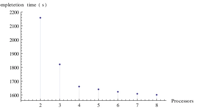
2 3 4 5 6 7 8 Processors 1600
1700 1800 1900 2000 2100 2200
[image:14.595.145.476.106.288.2]Completetion timeHsL
Figure 3: Completion time for deriving the expansion of a complex model using from 2 to 8 processors.
ruleModel={Q[0]->aj[{0}],Q[1]->-aj[{0}],Q[2]->bj[{1}]}};
A small number (e.g., 4) of Picard iterations is sufficient for a good approximation (see Papavasiliou and Ladroue 2010). An optional parameter is the maximum word length of the iterated integrals.
Running the algorithm with these parameters, we obtain the expansion, which is a weighted sum of 676 iterated integrals and already has aByteCount (size) of 504’768. Its expectation is a much smaller expression:
at−a
2t2
2 + a3t3
6 − a4t4
24 + 1 4a
3b2t4− 7
20a
4b2t5+ 61
360a
5b2t6− 1
24a
6b2t7+ 17
140a
5b4t7
1 192a
7b2t8− 21
160a
6b4t8+157a7b4t9
3024 −
17a8b4t10 2800 +
43a7b6t10 1800 −
1 100a
8b6t11
This is confirmed by the previous implementation of Picard iteration with the simple code:
P0[x_] := a (1 - x); P1[x_] := b x^2;
expansion = Picard[{P0, P1}, 0, 4]; ExpSBM[t, expansion]
However, if we now set the initial value to an arbitraryy0instead of 0, the stochastic expansion
contains a much larger number of terms. It is calculated in the same manner usingQas:
ruleModel={Q[0]->a(1-y0)j[{0}]+by0^2j[{1}],
Q[1]->-aj[{0}]+2by0j[{1}],Q[2]->bj[{1}] };
left in a file whose entries are parts of the linear combination. Thus, it is possible to, for example, compute the expectation of the expansion without having to store it in memory at any point. Moreover, while computationally expensive, these expansions can be calculated once in a general case and saved in a file for future application without having to recompute themde novo.
The notebook DistributedExpansion.nb provides a few examples and validations of the approach.
Figure 3 shows how the performance changes with the number of processors used. There is an increase in speed until the performance reaches a plateau. This is due to an input/output bottleneck which takes a constant time (the collection of expression’ positions in a file, to be assigned to the different processors).
5. Conclusion
Stochastic expansions provide a local approximation of the solution of a stochastic (or deter-ministic) differential equation. They can be used for a variety of applications, from simulation to parameter estimation. However, as the number of terms grows exponentially with the de-sired precision, they can rapidly become unwieldy to manipulate.
We presented a new way of calculating these expansions that bypasses the limitation of the usual approach,viaa reparametrization of the problem and the parallelization of the computa-tion. We have shown that in a simple example our method was able to compute the expansion when a direct approach failed. We also presented two new approaches for efficiently deriving the shuffle product of two iterated integrals and the expectation of an iterated integral, when the drivers are time and Brownian motion.
So far, our approach has been implemented for one-dimensional differential equation. How-ever, the theoretical foundation for the multi-dimensional case is available, as presented in Section 2.3. Now that the computing requirements have been alleviated, an implementation for the general case is possible. Stochastic expansions will then be available for more complex systems.
Acknowledgments
This work was funded by the EPSRC (EP/H019588/1, ‘Parameter Estimation for Rough Differential Equations with Applications to Multiscale Modelling’). We would like to thank the Mathematica newsgroup (comp.soft-sys.math.mathematica group) for their help and advice on file parallelization. We are also grateful to the reviewer for their suggestions and their help.
References
Kloeden PE, Platen E (1991). “Relations between Multiple Ito and Stratonovich Integrals.” Stochastic Analysis and Applications,9(3), 311–321.
Ladroue C (2010). “Expectation of Stratonovich Iterated Integrals of Wiener Processes.” ArXiv:1008.4033 [math.PR], URLhttp://arxiv.org/abs/1008.4033.
Lyons T, Qian Z (2003). System Control and Rough Paths. Oxford University Press.
Papavasiliou A, Ladroue C (2010). “Parameter Estimation for Rough Differential Equations.” ArXiv:0812.3102 [math.PR], URLhttp://arxiv.org/abs/0812.3102.
Tocino A (2009). “Multiple Stochastic Integrals withMathematica.” Mathematics and Com-puters in Simulation,79(5), 1658–1667.
Wolfram S (2003). The Mathematica Book. 5th edition. Wolfram Media.
Affiliation:
Christophe Ladroue, Anastasia Papavaviliou Department of Computer Science
University of Warwick
CV47AL, Coventry, United Kingdom
E-mail: [email protected],[email protected]
URL:http://www2.warwick.ac.uk/fac/sci/statistics/staff/academic/papavasiliou
Journal of Statistical Software
http://www.jstatsoft.org/published by the American Statistical Association http://www.amstat.org/
Volume 53, Issue 11 Submitted: 2010-08-25