Three-Dimensional Visualisation of Gas-water Two-phase Flow Based on Bubble Mapping Method and Size Projection Algorithm

Kun Li

, Qiang Wang

, Mi Wang

a_{Shanxi Key Laboratory of Signal Capturing and Processing, North University of China, Taiyuan, 030051, China} b_{School of Chemical and Process Engineering, University of Leeds, Leeds, LS2 9JT, UK}

c_{School of Chemistry, University of Edinburgh, Edinburgh, EH9 3FJ, UK}

A R T I C L E I N F O

Keywords:

Three-dimensional visualisation Gas-water pipelineflow Electrical impedance tomography Bubble mapping method Size projection algorithm

A B S T R A C T

Electrical impedance tomography (EIT) has been successfully applied on gas-waterflow applications, but it is incapable to identify small bubbles or the sharp gas-water interface of a large bubble due to its relatively low spatial resolution. A new visualisation approach, bubble mapping method (BM3D), offers a good 3D visualisation of bubble size and distribution. However, the empirical thresholding value method used in BM3D might meet a challenging from variousflow setups and conditions in practice. Recently, the size projection algorithm (SPA) was proposed to determine the closest thresholding value for each frame of tomogram by minimising projection error. In this paper, the performances of BM3D and SPA methods are individually analysed and evaluated. Then a new method based on the combination of BM3D and SPA methods is reported to achieve better visualisation of gas-waterflow, where the SPA is employed to determine the optimised thresholding values for BM3D method. Experiments are conducted to evaluate the proposed combination method for typical gas-water pipelineflow regimes, including horizontal stratified, bubble, plug, slug, annularflow regimes and vertical bubble, slug, annularflow regimes. The results are compared with the BM3D method, colour mapping method, and high-speed camera video recorded from a transparent chamber. A brief discussion on the effects of reconstruction algorithms and thresholding value for horizontal and verticalflows visualisation is also given.

1. Introduction

Gas-water two-phaseflow is a common and importantflow in many industries, where the flow visualisation is of significance for under-standing and predictingflow dynamics, process operation, analysis and design offlow control equipment [1,2]. The on-site inspection with a high-speed camera through a transparent chamber might be the most common and direct visualisation method to reveal the gas distribution in water [3–5]. However, this method is subject to the availability of the transparent chamber, transparency of continuousfluid. Moreover, high gas void fraction (over 10% [6]) affects the reliability of ob-servation. As an alternative technique, tomographic methods (including optical, ultrasonic or acoustic,γ/X-ray, microwave, resistive or capa-citive tomography), are highly considered as a promising technology because of providing 2D/3D images for various multiphasefluids with a feature of “seeing through”. Particularly, electrical impedance tomo-graphy (EIT) is a non-intrusive and cost-effective visualisation tech-nique with a high temporal resolution (sub-millisecond [7]), which can produce a stack of cross-section images for revealing the disperse phase

distribution in water continuous two-phase flows, where the phase difference in conductivity exists. However, tomograms generated by EIT are normally ambiguous with relatively low spatial resolution (up to 5% [8]), which is incapable of identifying very small bubbles and determining sharp gas-water interfaces. However, according to simpli-fied Maxwell relationship as expressed by Equation (1), EIT system could manage almost full gas volume fraction range (close 100%) for gas-water two-phaseflow [9] but not the gas-water boundary.

= −

+

σ σ

σ σ

c 2 2

2 mc

mc 1

1 (1)

where,cis the gas concentration,σ1andσmcare the water conductivity and reconstructed local conductivity, respectively.

Commonly, grey-level or colour palette based mapping methods [10] were employed for visualising gas-water distribution by con-verting the different values of gas concentration to different grey levels or colours based on predefined lookup tables. However, the converted images are limited in revealing flow characteristics sufficiently, and may vary greatly in human vision and machine perception because of

https://doi.org/10.1016/j.flowmeasinst.2019.101590

Received 23 April 2019; Accepted 5 July 2019

∗_{Corresponding author.}

E-mail address:[email protected](M. Wang).

Available online 10 July 2019

the differences from predefined lookup tables. Recently, a novel es-tablished method, called bubble mapping (BM3D) [11], enabled a good 3D visualisation of bubbles size and distribution in gas-water two-phase flow. The thresholding value used in BM3D is based on empirical knowledge, which has a potential challenge from variousflow setups and condition in practice. The SPA method [12] was proposed for imaging large bubbles by determining the optimised thresholding value for processing EIT tomogram of large bubbles, but did not perform well for imaging small bubbles. This paper reports a method for 3D visua-lisation of gas-water flow that utilises principles of bubble mapping method and apply thresholding values determined by the size projec-tion algorithm, providing an improvement visualisaprojec-tion quality on both small and large bubbles.

2. Methodology

Considering fully developed gas-waterflows, typicalflow regimes and associatedflow conditions are illustrated inFig. 1a and b in regard to horizontal and verticalflows respectively [1,13]. Except mistyflow regimes, the gas distributions at the cross-section of typical flow re-gimes can be characterized as three categories of (1) small bubbles (e.g. bubble regime, in tails of churn regime, etc.), or (2) only a large bubble (e.g. stratified, slug, plug or annular regimes), or (3) a large bubble surrounded with few small bubbles (e.g. slug, plug or churn regimes). Further, the category (3) could also be treated as (2) since the con-tribution from those few small bubbles to the local gas volume fraction and also to theflow regime visualisation can be ignorable according to the general flow principle [1,14]. With the assumption of ignoring small bubbles in the category (3), the size projection algorithm is em-ployed to visualise the distinctive large bubble as stated inflow cate-gories (2) and (3), while the bubble mapping method is employed to visualise the small bubbles in the category (1).

2.1. Bubble mapping method

The BM3D method [11] is a new established approach aiming at enhancing the capability of EIT to visualise gas-water pipeline flows. With the input of EIT reconstructed gas concentration tomogram, BM3D could transform a stack of cross-sectional tomograms into a collection of individual gas bubbles in the pipe, which reveals a vivid 3D visua-lisation of disperse gas phase distribution. The BM3D method is mainly based on a predefined lookup table indexed by bubble size and an en-hanced isosurface algorithm, whose major procedures are briefly in-troduced as follow:

(1) Re-meshing: According to the spatial resolution of EIT system and the small bubble size in real situation, the pipe space is re-meshed into coarser cube cells. Thereafter, the EIT reconstructed gas

concentration data are re-filled into the coarser cube cells with considering the actual gas velocity and data acquisition speed of EIT system.

(2) Bubble identification: After the re-meshing, two critical parameters or thresholding values,Tl(0.05, resulted from measurement error) and Tg (0.4, starting forming large bubble), are employed for identifying the bubble in each cube cell. If the gas concentration is belowTl, the cell is assumed being fully occupied by water. If the gas concentration is betweenTl andTg, a predefined lookup table transforms the reconstructed value (i.e. gas concentration in each cell) into a gas bubble whose volume fraction occupied in cube cell is equal to its gas concentration. However, if the gas concentration is aboveTg, the cell is assumed being fully occupied by gas, then an enhanced isosurface algorithm is employed to merge the neigh-boring cells with high gas concentration into a large bubble and to extract the boundary between gas bubble and water.

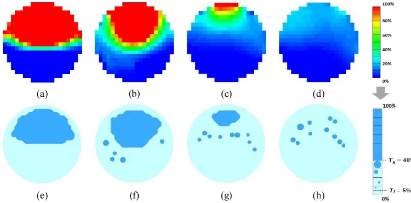
A set of existing concentration tomogram data collected at hor-izontal plugflow regime are used to evaluate the visualisation cap-ability of the BM3D method. The plugflow was generated on a gas-waterflow loop facility at the University of Leeds, where the superficial velocities of gas and water phases were 0.38 m/s and 1.02 m/s, re-spectively. The pipeline offlow loop is made of PVC tubes with an in-ternal diameter of 50 mm, and the concentration data were re-constructed by a commercial EIT system with imaging speed of 312.5 fps. On one hand, four frames of concentration tomograms at different points of plugflow are processed by BM3D method, where there is a large bubble, or a large bubble with small bubbles, or tail of a plug bubble with small bubbles, or small bubbles in the pipe cross-section. The cross-sectional images obtained from BM3D method and conventional colour mapping method are compared inFig. 2. On the other hand, 500 frames of concentration data were imported into BM3D software and processed for 3D visualisation. The visualisation results are compared with the conventional colour mapping method and the video recorded by a high-speed camera, as shown inFig. 3.

In Fig. 2, when only a large bubble exists in the cross-section (Fig. 2a and e), the BM3D result is similar to the image obtained from the conventional colour mapping method. However, when small bub-bles are introduced, the BM3D method can approximately reveal the distribution of large and small bubbles in water, while the colour mapping method has the quite limited capability on visualisation of small bubbles. In Fig. 3, a stack of cross-sectional tomograms are transformed and displayed as a series of individual large and small bubbles (Fig. 3c) by the BM3D method. And the BM3D result is com-pared with the image obtained from the colour mapping method and on-site video taken through a transparent chamber by a high-speed camera. The large plug bubbles are visualised by all three methods, while small bubbles are presented by cloud in on-site video and missing

Fig. 1.Generic two-phaseflow regimes maps [13].

in colour mapping-based image, but are highlighted in bubble mapping method. The results demonstrate the BM3D method is a good bubble-based 3D visualisation method with providing the key information, e.g. the size and shape, of both large and small bubbles, which is capable of improvingflow regime visualisation and visual recognition. However, the selection of thresholding valueTg(0.4) in BM3D method is based on empirical knowledge [15], which may meet a great challenging on imaging accuracy of large bubble in variation offlow setups and image reconstruction algorithms.

2.2. Size projection algorithm

The SPA method [12] is a new threshold-based image segmentation method for accurately extracting large bubbles in EIT tomogram, where the optimised thresholding value is machine-determined by a multi-step iterative process for distinguishing the gas bubble and water phase in EIT tomogram. In the SPA method, a projection error between EIT measured voltages and computed voltages of segmented image is em-ployed and minimised for approaching the optimised thresholding value, which means the minimal projection error should be reached when the segmented image is close to the real gas distribution. Once the optimal thresholding value is reached, the large bubble is extracted by converting the original EIT concentration tomogram to binary con-centration tomogram with the following Equation(2).

=⎧ ⎨ ⎩

≥

<

c k T c k T C(k) 1, ( )

0, ( ) sp

sp ₍₂₎

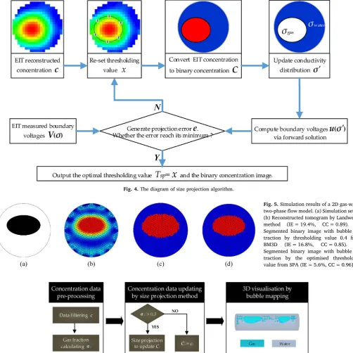
where,C(k)andc k( )are the gas concentration value ofk-th pixel in the updated tomogram and the original tomogram, respectively.Tspis the optimised thresholding value determined by the SPA method for the frame of cross-sectional tomogram. The principle of SPA method is il-lustrated inFig. 4.

In order to evaluate the accuracy of large bubble extraction by SPA method, a 2D gas-water two-phase model (i.e. a large bubble in water) was simulated in COMSOL software, as shown inFig. 5a. A typical 16-electrode EIT sensor and the adjacent sensing strategy were employed, which could generate 104 independent boundary voltages for solving inverse problem. Then the processes of image reconstruction and seg-mentation were conducted under a mesh with 1536 triangular pixels. As shown inFig. 5, the reconstructed tomogram (Fig. 5b) is obtained from Landweber method [16] and the binary images (Fig. 5c and d) are obtained from threshold-based image segmentation methods with re-spect to the empirical thresholding value 0.4 (i.e. in BM3D method) and the optimised thresholding value (i.e. in SPA method), respectively. Two evaluation criteria [17], i.e. relative image error (IE) and corre-lation coefficient (CC) between the setup model and reconstructed image or segmented image, are used to estimate the imaging accuracy of large bubble.

As shown inFig. 5, the sharp boundary of the large bubble is not clearly identified in EIT reconstructed tomogram, but explicitly ex-tracted by the BM3D and SPA methods with their corresponding thresholding values. Meanwhile, the bubble extracted from SPA method is more accurate than it extracted from the BM3D method, which de-monstrates the SPA performance of imaging large bubble is better than BM3D method. However, SPA method cannot identify the small bubbles in water since it is not sensitive to small bubbles. Therefore, SPA could only be used for imaging large bubble in each frame of EIT tomogram by the determination of the optimised thresholding value.

2.3. Combination method for 3D gas-waterflow visualisation

As illustrated in Section2.1 and 2.2, BM3D method can provide a good 3D visualisation of gas-waterflow with revealing large and small bubbles distribution, while it meets a theoretical challenge on the ac-curacy of imaging large bubbles in various flow regimes since the

Fig. 2.Cross-sectional images generated by conventional colour mapping methods (the top) and by BM3D method (the bottom) at different points of plugflow. In the pipeline cross-section, there is a large bubble ((a) & (e)), or a large bubble with small bubbles ((b) & (f)), or the tail of plug bubble with small bubbles ((c) & (g)), or small bubbles ((d) & (h)).

thresholding value of BM3D is a global fixed value. However, SPA method can provide the closest thresholding value for imaging large bubble in each frame of tomogram even it is not sensitive for small bubbles. According to a large scatter of data [1], large bubble starts being formed from small bubbles in pipeline when the gas fraction

reaches a certain thresholding value (0.3 corresponding to the experi-mental conditions in this paper), that is the large bubble will exist, and in contrast almost only small bubbles exist if gas fraction is below the

Fig. 4.The diagram of size projection algorithm.

Fig. 5.Simulation results of a 2D gas-water two-phaseflow model. (a) Simulation setup. (b) Reconstructed tomogram by Landweber method (IE = 19.4%, CC = 0.89). (c) Segmented binary image with bubble ex-traction by thresholding value 0.4 from BM3D (IE = 16.8%, CC = 0.85). (d) Segmented binary image with bubble ex-traction by the optimised thresholding value from SPA (IE = 5.6%, CC = 0.96).

Fig. 6.The schematic diagram of combination procedure.

Fig. 7.The arrangement of test section at TUV NEL.

Table 1

Theflow conditions for typical horizontal gas-waterflow regimes.

vsg(m/s) vsw(m/s) Qgas(m3/ h)

Qwater(m3/ h)

GVF (%) Observedflow regimes

0.114 0.026 12.887 2.939 81.67 Stratifiedflow 0.064 1.232 7.235 139.27 4.94 Bubbleflow 0.136 0.754 15.373 85.232 15.31 Plugflow 0.541 0.353 61.155 39.903 60.54 Slugflow 4.483 0.066 506.76 7.461 98.54 Annularflow

thresholding value. The combination of BM3D and SPA is considered to overcome the limits in each method, where SPA is employed to de-termine the optimised thresholding value for BM3D method when large bubble exists. Considering the procedures of two methods, the con-centration tomogram data need to be processed by SPA before being imported into BM3D software. The schematic diagram of combination procedures is depicted inFig. 6.

Since unavoidable noise in measurement, the gas concentration value might contain abnormal data in tomogram, such as negative value, and it should befiltered out and thus producing a meaningful gas concentration region, i.e.[0.0, 1.0]. Then the mean gas fraction αi is calculated as the average of gas concentration value at each pixel of a tomogram, as expressed in Equation(3), which is a decisive factor for the optimised threshold determination by employing SPA method. If the mean gas fraction of i-th frame tomogram is upper than 0.3, the frame of concentration tomogram ci is converted to a binary con-centration tomogramCiby Equation(2), otherwise letCi=ci. Finally, the BM3D method is employed to transform the updated concentration tomogram dataCinto a 3D visualisation of gas-waterflow by revealing the distribution of both large and small bubbles.

∑

=

=

c k N αi ( ( )/ )

k N

i

1 (3)

where,αiis the mean gas fraction of thei-th frame tomogram.c ki( )is the gas concentration value of thek-th pixel in thei-th frame tomogram. Nand the subscriptiare the total pixel number and the frame number of gas concentration tomogram.

3. Evaluation

Before the proposed combination method is evaluated, it should be clarifiedfirstly that the objective of the study is to enhance the 3D vi-sualisation of gas-waterflow by replacing thefixed thresholding values in BM3D with optimised thresholding values determined by SPA method. The accuracy of thresholding values determined by the SPA method was demonstrated in paper [12] and Section2.2in this paper. The 3D gas-waterflow visualisation results of proposed combination method are compared with the BM3D method, along with corre-sponding images from colour mapping method and high-speed camera video. For the convenience in following text, the video method, the colour mapping method, the BM3D method, and the proposed combi-nation method (i.e. BM3D with SPA) are abbreviated as VD, CM, BM and BS, respectively. In addition, it is worth pointing out that the BM and BS visualisation results include pipe wall.

3.1. Visualisation of gas-waterflow in horizontal pipeline

The horizontal gas-water flow experiments were conducted using gas-water facilities at TUV NEL (National Engineering Laboratory at Glasgow, UK). The arrangement of test section is depicted inFig. 7. ITS V5R system [18] was employed for collecting EIT tomogram data with 312.5 dual-frames per second (dfps). Meanwhile, a high-speed camera was also installed to record theflow structures through a transparent chamber for comparison. The gas phase was nitrogen with 0mS/cm

conductivity and 1.25 kg/m3density, and the water phase was salty water with 33.5mS/cmconductivity and 1049.1 kg/m3density. Since the involved facilities can produce gas-waterflow with 0%–100% GVF, it was able to generate commonflow regimes in horizontal pipeline. The superficial gas and water velocities were controlled to achieve certainflow conditions for generating typical horizontalflow regimes (including stratified, bubble, plug, slug and annular regimes). Theflow conditions referenced by testing facilities are listed inTable 1.

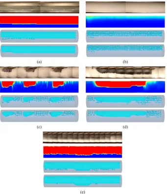
The resultant visualisation results of the four methods are shown in Fig. 8. The VD images were generated by connecting several screen-shots, and the gas and water phases in the CM images were represented by red and blue colours. For the stratifiedflow inFig. 8a, theflow regime is clearly recognised by four images. Only in the BM image, few small bubbles exist at the gas-water interface. For the bubbleflow in Fig. 8b, the small bubbles cannot be identified in the VD and CM images, but clearly visualised in the BM and BS images. When it comes to the plug and slugflow inFig. 8c and d, the large bubbles can be located in all images. However, the small bubbles are missing in the VD and CM images, but clearly visualised in the BM and BS images. It is noted to point out that the proposed combination method only reveals the large bubble visualisation with eliminating the small bubbles at the existence position of a large bubble. For the annularflow inFig. 8e, the thin waterfilm at the top position is not revealed in the CM, BM and BS images since it is too thin to be identified by EIT system. Comparing the BM and BS visualisation results, the only difference is the elimination of small bubbles at the existence position of large bubble, because the SPA method ignores the existence of few small bubbles for achieving accu-rate visualisation of large bubbles in proposed combination method.

3.2. Visualisation of gas-waterflow in vertical pipeline

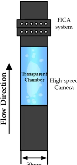
The vertical gas-waterflow experiments were performed on upward gas-water flow loop facilities with 50 mm-diameter pipeline at OLIL (Online Instrumentation laboratory) in the University of Leeds. The arrangement of test section is depicted inFig. 9, and FICA system [8] is employed for collecting EIT tomogram data with 1000 dual-frame per second (dfps), and a high-speed camera is utilised as well. The gas phase was compressed air with 0mS/cmconductivity and 1.29 kg/m3_density,

and the water phase was tap water with 0.35mS/cmconductivity and 1000 kg/m3 density. The superficial gas and water velocities were controlled to achieve certain flow conditions for generating typical verticalflow regimes (including bubble, slug and annular regimes). The flow conditions referenced by testing facilities are listed inTable 2.

The resultant visualisation results of the four methods are shown in Fig. 10. For the bubble flow inFig. 10a, except the CM image, all images visualised the bubbles distribution by clearly showing the bubbles size and location. For the slugflow inFig. 10b, the VD image can approximately estimate the location of slug bubble, while it can

Fig. 9.The arrangement of test section at OLIL.

Table 2

Theflow conditions for typicalflow regimes.

vsg(m/s) vsw(m/s) Qgas(m3/ h)

Qwater(m3/ h)

GVF (%) Observedflow regimes

0.085 0.878 0.600 6.199 4.94 Bubbleflow

0.51 0.57 3.601 4.024 60.54 Slugflow

18.42 0.035 130.05 0.247 98.54 Annularflow

Fig. 10.Visualisation results on typical verticalflow regimes (Flow direction from bottom to top). Each set of images (from left to right) are obtained from high-speed camera video (VD), colour mapping method (CM), bubble mapping method (BM) and proposed combination method (BS), re-spectively. (a) Bubbleflow regime. (b) Slug

flow regime. (c) Annularflow regime.

hardly estimate the exact bubble size and shape because of too many small bubbles. The CM image reveals the approximate shape and lo-cation of slug size, but the sharp bubble boundary and small bubbles cannot be revealed. The BM and BS images illustrate the bubble loca-tion, shape, sharp boundary and small bubbles. However, the size of slug bubble in the BS image is larger than in the BM image, and the small bubbles at the position of slug bubble are eliminated. For the annularflow inFig. 10c, both the VD and CM images show theflow regime, but they cannot determine the size of annular air-core. How-ever, the air-core size is clearly shown in the BM and BS images, where the size of annular air-core in the BS image is larger than the BM image, which more closely reflect the true phenomenon of annularflow regime with a thin layer of water. Comparing the BM and BS visualisation re-sults, the proposed combination method reveals a bigger size of large bubble and eliminates the existence of small bubbles at the position of large bubble when the large bubble exists. This is because the thresh-olding values determined by SPA in the proposed combination method are smaller than in BM3D, and SPA method ignores the existence of few small bubbles at the large bubble position for accurately visualising large bubble.

4. Discussions

4.1. Impact of tomographic algorithms on visualisation

The aim of EIT tomographic algorithms in gas-water two phaseflow visualisation is to determine the unknown distribution of gas phase based on the measured boundary voltages. Due to the so-called “soft-field”effect and ill-posed problem, the expected precision is incapable from current inverse solution. There are many tomographic algorithms developed for EIT, which can be classified into two categories, quali-tative non-iterative algorithms and quantiquali-tative iterative algorithms [19]. As the fast speed is required for online gas-waterflow measure-ment and visualisation, only qualitative non-iterative algorithms (i.e.

SBP and MSBP algorithms) are discussed in this paper.

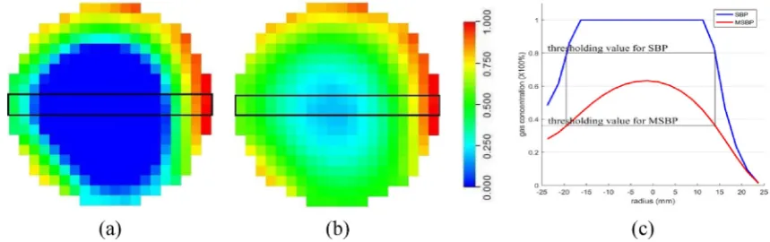
SBP algorithm was firstly produced by Kotre [20] based on the principle of linear back-projection (LBP). Later, the modified SBP al-gorithm (MSBP) was proposed by Wang [21] based on an approxima-tion of inverse relaapproxima-tion, i.e.1+x≈1/(1−x)atx<1, which extends the application range further. Actually, the nonlinear approximation should be satisfied byx→0in mathematics. But the conditionx<1 makes MSBP algorithm work better to speed up the inverse process of imagingflow in vertical layout since the disperse phase has a more homogeneous distribution in verticalflow. It was further demonstrated that the MSBP algorithm has a better correlation of gas concentration and the conductivity ratio than the SBP algorithm [9]. As shown in Fig. 11, a comparison of SBP and MSBP results on vertical slugflow is conducted. The SBP and MSBP show a similar distribution trend in conductivity tomogram, as shown inFig. 11a and b. But according to the comparison of gas concentration profiles in Fig. 11c, different thresholding values are needed for extracting the same bubble from SBP and MSBP images reconstructed with same measured boundary vol-tages, which is the impact of tomographic algorithms on the thresh-olding value selection for verticalflow visualisation.

However, the disperse phase in horizontalflow layout presents a highly heterogeneous, and the reconstructed conductivity change ratio might be close to1or even far beyond1. Therefore, the condition of MSBP will be no longer satisfied in principle, and the reconstructed conductivity tomogram from MSBP will show few pixels having ab-normal value. As shown inFig. 12, a comparison of SBP and MSBP results on horizontal plugflow is conducted, which clarifies that the MSBP is not applicable for imaging horizontal pipelineflow. Therefore, the SBP algorithm is employed to visualising horizontal gas-waterflow, while the MSBP algorithm is employed to visualising the vertical gas-waterflow in this work.

tomogram. (b) MSBP reconstructed conductivity tomogram. (c) Gas concentration profiles corresponding to the tomograms (a) and (b).

4.2. Impact of thresholding values on bubble mapping

In the proposed combination method, the size projection algorithm determines the optimised thresholding values for extracting large bubble's boundary when a large bubble exists. As the mean gas fraction is less than 0.3, the SPA method will not be employed, which remains

the original concentration tomogram data to form small bubbles using the BM3D method.

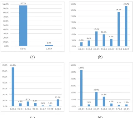
For the horizontal pipelineflow, the thresholding values determined by SPA method are statistically analysed, and its histograms of prob-ability distribution are given in Fig. 13. Although the thresholding values used in the proposed method are quite different with the

Fig. 13.Histograms of probability distribution of thresholding value. (a) Stratifiedflow regime. (b) Plugflow regime. (c) Slugflow regime. (d) Annularflow regime.

Fig. 14.Histograms of probability distribution of thresholding value. (a) Slugflow regime. (b) Annularflow regime.

thresholding values used in BM3D method, the 3D visualisation results of large bubbles from two methods are little difference, as shown in Fig. 8. That is because the employment of SBP algorithm makes the artefacts zone in reconstructed tomogram very narrow, as shown in Fig. 12c. Therefore, it is demonstrated that the thresholding values used in BM3D method for horizontalflow do not have a significant impact on the quality of visualisation.

For the vertical pipelineflow, the thresholding values determined by SPA method are also statistically analysed, and its histograms of probability distribution are given inFig. 14. Most of the thresholding values used in the proposed method are smaller than the thresholding value used in BM3D method, which results in the significant difference of large bubble visualisation in two methods. That is due to the em-ployment of MSBP algorithm making the artefacts zone in reconstructed tomogram relatively wide, as illustrated inFig. 11b and c. Therefore, it is demonstrated that the thresholding values used in BM3D method for verticalflow have a significant impact on the quality of visualisation.

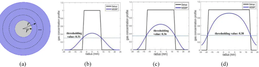
Further, a simulation is conducted to investigate the accurate thresholding values for extracting the real bubbles with different size in MSBP reconstructed tomograms. A sequence of setups (Fig. 15a) were modeled according to the cross-sectional configuration of a large bubble in vertical flow, where the background phase is tap water (0.35mS/cm) and the disperse phase is air (0mS/cm). A typical 16-electrode EIT sensor and adjacent sensing strategy were employed to generate the 104 independent boundary voltages for solving the inverse problem. The bubbles were reconstructed by MSBP algorithm and compared with the real setup bubbles based on the COMSOL simulation data, as shown in Fig. 15b~d, which demonstrates that the thresh-olding values for extracting the reconstructed bubbles with different size are different. Therefore, thefixed thresholding value (i.e. 0.4) in BM3D method tends to underestimate the size of the slug bubble or annular air-core in vertical flow. In addition, the artificial effect of blurry boundary in MSBP reconstructed results is not a narrow zone, as shown inFig. 15b~d, which will be mistakenly converted into small bubbles at the boundary of a large bubble.

5. Conclusions

In this paper, a combination method utilises the size projection al-gorithm (SPA) to enhance the bubble mapping based 3D visualisation of gas-in-water two-phase flows. With the reasonable assumption, the large bubble's boundary is extracted by the SPA method determined optimised thresholding values, while small bubbles are formed from the original concentration tomogram data using the bubble mapping method. The evaluation results demonstrate a better visualisation per-formance of the proposed combination method. For horizontal gas-waterflow, the thresholding value in BM3D method does not affect the visualisation very much. For vertical gas-waterflow, the BM3D method tends to underestimate the large bubble size, while the proposed combination method offers a better estimation. In addition, the artifi -cial effect of blurry boundary from conventional tomographic algorithm

makes BM3D method mistakenly create small bubbles nearby a large bubble. With the employment of the SPA method, this effect can be fully removed, which are revealed in images from both vertical and horizontalflow layouts.

Acknowledgments

The authors would like to express their gratitude for the support from the Chinese Scholarship Council (CSC) and the School of Chemical and Process Engineering, who made Mr. Li's study at the University of Leeds possible. This work is also funded by the Engineering and Physical Sciences Research Council (EP/H023054/1, IAA (ID101204) and the European Metrology Research Programme (ENG58-MultiFlowMet) project‘Multiphaseflow metrology in the Oil and Gas production’, which is jointly funded by the European Commission and participating countries within Euramet and the European Union. References

[1] S. Levy, Two-phase Flow in Complex Systems, John Wiley & Sons, 1999. [2] C.E. Brennen, Fundamentals of Multiphase Flows, Cambridge University Press,

2005.

[3] R. Maceiras, E. Álvarez, M.A. Cancela, Experimental interfacial area measurements in a bubble column, Chem. Eng. J. 163 (3) (2010) 331–336,https://doi.org/10. 1016/j.cej.2010.08.011.

[4] Y.M. Lau, N.G. Deen, J.A.M. Kuipers, Development of an image measurement technique for size distribution in dense bubblyflows, Chem. Eng. Sci. 94 (5) (2013) 20–29,https://doi.org/10.1016/j.ces.2013.02.043.

[5] Y. Fu, Y. Liu, 3D bubble reconstruction using multiple cameras and space carving method, Meas. Sci. Technol. 29 (7) (2018) 075206, ,https://doi.org/10.1088/ 1361-6501/aac4aa.

[6] H.M. Prasser, D. Scholz, C. Zippe, Bubble size measurement using wire-mesh sen-sors, Flow Meas. Instrum. 12 (4) (2001) 299–312, https://doi.org/10.1016/s0955-5986(00)00046-7.

[7] M. Wang, Y. Ma, N. Holliday, Y. Dai, R.A. Williams, G. Lucas, A high-performance EIT system, IEEE Sens. J. 5 (2) (2005) 289–299,https://doi.org/10.1109/JSEN. 2005.843904.

[8] M. Wang, F.J. Dickin, R. Mann, Electrical resistance tomographic sensing systems for industrial applications, Chem. Eng. Commun. 175 (1) (1999) 22,https://doi. org/10.1080/00986449908912139.

[9] J. Jia, M. Wang, Y. Faraj, Evaluation of EIT systems and algorithms for handling full void fraction range in two-phaseflow measurement, Meas. Sci. Technol. 26 (1) (2015) 015305, ,https://doi.org/10.1088/0957-0233/26/1/015305.

[10] C.D. Hansen, C.R. Johnson, The Visualization Handbook, Publisher: Elsevier, 0-12-387582-X, 2005.

[11] Q. Wang, X. Jia, M. Wang, Bubble mapping: three-dimensional visualisation of gas-liquidflow regimes using electrical tomography, Meas. Sci. Technol. (2019) in press https://doi.org/10.1088/1361-6501/ab06a9.

[12] K. Li, Q. Wang, M. Wang, Imaging of a distinctive large bubble in gas-waterflow based on size projection algorithm, Meas. Sci. Technol. (2019) in presshttps://doi. org/10.1088/1361-6501/ab16b0.

[13] S. Corneliussen, J.P. Couput, E. Dahl, E. Dykesteen, K.E. Frysa, E. Malde, H. Moestue, P.O. Moksnes, L. Scheers, H. Tunheim, Handbook of multiphaseflow metering, Revision 2 (2005) 82-91341-89-3.

[14] M.M. Razzaque, Bubble size distribution in a large diameter pipeline, Proc. of IMEC & APM, Dhaka, 2005.

[15] M. Wang, X. Jia, M. Bennett, R.A. Williams, Flow regime identification and op-timum interfacial area control of bubble columns using electrical impedance ima-ging, 2nd World Congress on Industrial Process Tomography, 2001, pp. 726–734. [16] W.Q. Yang, D.M. Spink, T.A. York, An image-reconstruction algorithm based on

Technol. 10 (11) (1999) 1065–1069https://iopscience.iop.org/article/10.1088/ 0957-0233/10/11/315/meta.

[17] W.Q. Yang, L. Peng, Image reconstruction algorithms for electrical capacitance tomography, Meas. Sci. Technol. 14 (1) (2002) R1–R13https://iopscience.iop.org/ article/10.1088/0957-0233/14/1/201/meta.

[18] J. Jia J, M. Wang, H.I. Schlaberg, H. Li, A novel tomographic sensing system for high electrically conductive multiphaseflow measurement, Flow Meas. Instrum. 21 (3) (2010) 184–190https://www.sciencedirect.com/science/article/pii/ S0955598610000026.

[19] Z. Cui, Q. Wang, Q. Xue, W. Fan, L. Zhang, Z. Cao, B. Sun, H. Wang, W.Q. Yang, A review on image reconstruction algorithms for electrical capacitance/resistance tomography, Sens. Rev. 36 (4) (2016),https://doi.org/10.1108/SR-01-2016-0027. [20] C.J. Kotre, EIT image reconstruction using sensitivity weightedfiltered

back-pro-jection, Physiol. Meas. 15 (1994) A125–A136https://iopscience.iop.org/article/10. 1088/0967-3334/15/2A/017/meta.

[21] M. Wang, Inverse solutions for electrical impedance tomography based on con-jugate gradients methods, Meas. Sci. Technol. 13 (1) (2001) 101–117https:// iopscience.iop.org/article/10.1088/0957-0233/13/1/314/meta.