Prediction for Corrosion Status of the Metro Metal Materials in the Stray Current Interference

Int. J. Electrochem. Sci., 8 (2013) 5314 - 5329

International Journal of

ELECTROCHEMICAL

SCIENCE

www.electrochemsci.org

Prediction for Corrosion Status of the Metro Metal Materials in

the Stray Current Interference

Yu-Qiao Wang, Wei Li*, Shao-Yi Xu*, Xue-Feng Yang

School of Mechanical and Electrical Engineering, China University of Mining and Technology, Xuzhou City, Jiangsu Province, P.R. China, 221116

*

E-mail: [email protected]; [email protected]

Received: 10 February 2013 / Accepted: 13 March 2013 / Published: 1 April 2013

The metro metal materials have serious electrochemical corrosion in the stray current interference, and the corrosion status is characterized by the polarization potential offset value of the metal materials to the reference electrodes. Due to the limited number of the reference electrodes, it is necessary to predict the corrosion status of the metal materials in the area without reference electrodes. Firstly, it is concluded that the corrosion is electrochemical by analyzing the corrosion mechanism of the metal materials in the stray current interference. Secondly, characterization parameters and influence parameters of the corrosion status can be acquired by investigating the corrosion mechanism. Thirdly, the nonlinear mapping between characterization parameters and influence parameters is approximated using a Radial Basis Function (RBF) neural network. The node number of RBF network hidden layer is determined by Rival Penalized Competitive Learning (RPCL) algorithm, to form the complete RBF network. The key parameter values of the RBF network are obtained by Quantum Particle Swarm Optimization (QPSO) algorithm. Finally, according to the corrosion data from Nanjing metro Line 1 in China, the RBF prediction model is established and the prediction performance is illustrated. The results show that RBF model can accurately predict the corrosion status of the metro metal materials, and the application of RPCL algorithm and QPSO algorithm can improve the predictive ability of RBF model.

Keywords: Stray current; Metal materials; Corrosion status; RBF model

1. INTRODUCTION

shortening the service life of the buried metal pipeline and armored cable, but also reducing the strength and durability of the metro main structure [1, 3-6]. Therefore, it is essential to assess the corrosion status of metro metal materials in the stray current interference.

The metal material corrosion status is usually characterized by polarization potential offset value of the metal materials respect to the reference electrodes [3, 7-10]. The reference electrode is embedded in the vicinity of the metal materials. However, the metal material corrosion status cannot be assessed in the area, which is far away from the electrode embedded point. If a mathematical model of the polarization potential offset value and the impact factors can be obtained, the corrosion status of metal materials will be predicted, especially in the area without the reference electrodes, according to the corrosion data of the metal materials near the electrode embedded point.

There are few studies on the prediction method of metal material corrosion status in the stray current interference. The Back Propagation (BP) neural network is only the mentioned prediction method [3], where the soil resistivity, the depth of the metal materials and the polarization potential offset values are regarded as the input parameters and the stray current density is regarded as the output parameter of BP network. Although the stray current density can directly characterize the metal material corrosion status, the real-time measurement of the stray current density is very difficult in metro [11-15]. Therefore, the metal material corrosion status is characterized by measuring the polarization potential offset value. Some researches show that the polarization potential offset value is related to traction substation distance, rail longitudinal resistance, rail voltage and resistance between the rails and the metal materials [11-14, 16-21].

BP network and RBF network have been widely studied as two typical feed forward networks. It has been proved that BP network is worse than RBF network in the convergence speed and approximation ability, which can approximate arbitrary nonlinear function at arbitrary precision [22-24]. The RBF network is composed of input layer, hidden layer and output layer, which need to determine the number of hidden layer nodes and the key parameters value of the network, including RBF center value, width, connection weight between hidden layer and output layer. The RPCL algorithm makes the redundant units away from the input sample space using the rejection mechanism of suboptimal unit, realizing the automatic selection for the number of cluster and regulating effectively the number of the hidden layer nodes [25-26]. The QPSO algorithm can make particles explore the global optimization in the feasible solution space, which does not need feature information of problem. Therefore, the QPSO algorithm can be used to solve the key parameters of RBF network

[27-29].

2. CORROSION MECHANISM OF METAL MATERIALS IN STRAY CURRENT INTERFERENCE

The common corrosion modes of metal materials mainly include: general corrosion and pitting corrosion in metro, while stray current corrosion is a kind of pitting corrosion [15], which is classified as electrochemical corrosion. It has the oxidation-reduction reaction of the anodic and cathode process.

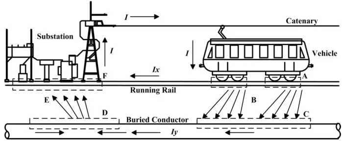
Stray current corrosion mechanism of the metal materials is that Fe at lower potential loses electrons and is oxidized to Fe2+, while H+ or O2 at higher potential captures an electron and is reduced. In stray current interference, the metal material corrosion has a remarkable characteristic that the negative potential region on metal materials is called the cathode, where stray current flows into the metal materials, and the positive potential region is regarded as the anode, where stray current flowing out. Moreover, the anode and cathode regions are separated from each other [1, 15]. Stray current and its corrosion position in metro are shown in Figure 1, where I is the traction current, Ix and

Iy is the negative current and stray current, respectively.

Figure 1. Schematic diagram of stray current corrosion in metro

According to the figure 1, the stray current path in metro can be summarized as two corrosion cell in series:

The First Cell: A Rail in the vehicle position (anode) → B Ballast bed or soil → C Buried conductor (cathode)

The Second Cell: D Buried conductor (anode) → E Ballast bed or soil → F Rail in the traction substation (cathode region)

Fe and the surrounding electrolyte generate anodic process electrolysis when stray current flowing out from the anode regions (A and D in Figure 1). The oxidation-reduction reaction can be summarized as follows:

(1) The reaction is hydrogen evolution corrosion taking H+ as the depolarizing agent when the surrounding electrolyte is acidic (PH < 7). The corrosion reaction equations are as follows:

Anode: 2Fe → 2Fe2+ + 4e

(2) The reaction is oxygen-absorbed corrosion taking O2 as the depolarizing agent when the surrounding electrolyte is alkaline (PH ≥ 7). The corrosion reaction equations are as follows:

Anode: 2Fe → 2Fe2+ + 4e

-Cathode: O2 + 2H2O + 4e- → 4OH- (Aerobic alkaline environment)

The hydrogen evolution and oxygen-absorbed corrosion typically generate Fe(OH)2. Some of Fe(OH)2 are further oxidized to form Fe(OH)3 or brown Fe(OH)3•2xH2O on the metal materials surface, while Fe (OH)3 can further produce Fe3O4.

3. CHARACTERIZATION PARAMETER AND INFLUENCE PARAMETERS OF THE CORROSION STATUS

In the stray current interference, the corrosion amount of metal materials obeys Faraday's law in terms of the stray current corrosion mechanism:

WKit (1)

where W is the corrosion amount of metal materials, kg; K is the metal electrochemical equivalent , kg / (A · s); i is stray current flowing out of the anode, A.

M K

nF

 (2)

where M is molar weight, kg / mol, and the molar weight of Fe is 5.5847×10-4 kg / mol; n is the number of the lost valence electrons in the oxidation process; F is the Faraday constant, and 1 F = 96485 C.

According to Eq. (1) and (2), the metal electrochemical equivalent k is constant in a specific corrosive environment. The stray current i directly characterize the corrosion status of metal materials, but the stray current is difficult to measure directly in metro. The metal material corrosion status is only characterized by the indirect indicator, which is the polarization potential offset value caused by the stray current.

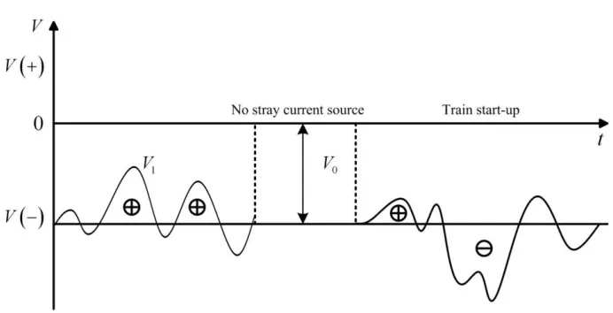
The long-acting reference electrode Cu/CuSO4 has been used to measure the polarization potential. Polarization potential distribution between the metal materials and the reference electrodes exhibits a stable value without the stray current interference, and we call the stable potential is the natural ontology potential V0. If the metal materials are interfered with the stray current, the measured potential V1 deviates from the natural ontology potential V0 in the positive or negative direction. We define the polarization potential offset value as V2, where V2 = V1 - V0. Polarization potential curve of the metal materials to the reference electrodes is illustrated in Figure 2.

The stray current is proportional to the distance of traction substations and the longitudinal resistance of rails, while it is inversely proportional to the substations output voltage and the resistance between the rails and metal materials. Therefore, the traction substation distance l, rail longitudinal resistance Rt, rail voltage U and the resistance Rg between the rail and metal materials are regarded as the influence parameters of the metal material corrosion status.

4. CORROSION STATUS PREDICTION MODEL

The influence parameters l, Rt, U and Rg are used as the input vectors of RBF neural network, while the characterization parameter V2 is used as the output vector. The nonlinear mapping relationship between the input vectors and output vector is approximated by RBF neural network. The metal material corrosion status is predicted based on the mapping relationship. The RBF network is composed of input layer, hidden layer and output layer, which need to determine the number of hidden layer nodes M and the key parameters value of the network, including RBF center value C, width, connection weight W between hidden layer and output layer. Therefore, the number M can be obtained by RPCL algorithm and the network parameters C, , W can be trained based on QPSO algorithm.

4.1 RBF Network

The input vector number of RBF neural network N is equal to 4, and the output vector number Z is equal to 1. The input vector is mapped directly to the hidden layer space, that is, the connection weight between input layer and hidden layer is 1. There are i groups of the corrosion samples Si = (Xi,

Vi), where i=1, 2, …, P, Xi and Vi are N dimensional and Z dimensional column vector respectively.

The activation function of the hidden layer nodes adopts M dimensional radial basis function, which is given as [22-23, 30]:

 





j i i Cj j M

 X   X   L (3)

where Cj is the center value of the radial basis function, and  is distance measure, which is

generally selected as Euclidean distance. The output of RBF network can be expressed as

1

ˆ M _{, 1, 2, ,}

d j jd d j

V w d Z



where wjd is the connection weight between the hidden layer node and the output layer node,

and d is the threshold value of the output layer node. The radial basis function usually selects Gauss distribution function [24], which is described as

 

where j is width of the radial basis function, determining the general shape of the radial basis function.

4.2 RPCL Algorithm

The hidden layer node number M is confirmed by RPCL algorithm. Corrosion samples are

 

P i i 

S S . The initial clustering center is Wj = (Wj1, …, Wj(N+Z))T, with j = 1, 2, …, k, k is the preset

number of the clustering centers. The learning rates of winning unit c and suboptimal unit r are c and r

 respectively. Based on RPCL algorithm, solving the number M has the following steps [25-26]: Step 1: Initializing the learning rates c

 

 

 

Step 2: Randomly selecting sample Si from S, with j = 1, 2, …, k.

2 2 1 2 2 1 ,

1, if such that min 1, if such that min 0, otherwise

c i c p i p

p k

j

r i r p i p

p k p c

j c

u _{j r}

          _{   }           

S W S W

S W S W (6)

where

 

 

1 G

j j j

t

n t n t





_

 , n tj

 

Step 3: Modifying the clustering center value as









,

,

0, otherwise

c i c

j r i r

j c

W j r

             S W

S W (7)

Step 4: Setting t = t + 1, if t < G, Step (2) and (3) will be executed.

Step 5: Comparing the length Wj of the clustering center vector Wj with the threshold value, which is _min and _max. The hidden layer node number M is equal to the number of the center vectors during the range of _min  W_j  _max.

4.3 Parameters Adjustment Using QPSO Algorithm

Step 1:

The feasible solution of the problem is characterized by the particle, which is constituted by the RBF network parameters C,  and W in the search space of QPSO algorithm. The network topology is N × M × Z. Assuming that the population of QPSO algorithm is X(t), namely X(t) = (X1, …, XM, X(M+1),

…, XM×(N+1), X M×(N+1)+1, …, XM×(N+Z+1)), where (X1, …, XM), (X(M+1), …, XM×(N+1)) and (X M×(N+1)+1, …,

XM×(N+Z+1)) are C,  and W, respectively, and t is iterations.

Assuming that the number of particles in X(t) is R and Xi(t) = (xi1(t), …, xiD(t)), where 1 ≤ i ≤

R, D = M × (N + Z + 1). The optimal position of the particle is expressed as Pi(t) = (pi1(t), …, piD(t)).

The optimal position of the population is expressed as Pg(t) = (pg1(t), …, pgD(t)).

Randomly generating the initial population, and then each particle converges to the local attraction point Li = (l i1, …, l iD) to ensure the convergence of QPSO algorithm. Li is as follow:

 

 





 

ij j ij j gj

L t   p t    p t (8)

where  j c r1 1j





2

c are the acceleration factors, which usually taken c c1= 2.

The particle behavior of QPSO algorithm conforms to quantum dynamics, depicting the particle position by the wave function and determining the status changes of particles from the Schrodinger equation [27-28]. Assuming that each particle moves in a δ potential well which regards the local attraction point Li as centers, the specific location of particle in δ potential well depends on a

probability density function F(x). Moreover, the QPSO algorithm has the best performance when F(x) is a quadratic function. Hence, F(x) is gained by solving the Schrodinger equation.

 

ij

F x e  (9)

where d is the length of δ potential well, which determines the particle search range. The iteration equation of particle position depicted in Eq. (10) is acquired using the Monte Carlo stochastic simulation method.

 

 

In 1 , 0,1

2 ij ij

d

x L  u u: U (10)

The mean optimal position mbest is introduced to preferably regulate the length d, which is

defined as the mean value of all particles optimal position.

 

 

 

 

1 1 1

1 1 1

, , ,

R R R

best i i iD

i i i

m t p t p t p t

R  R  R 

 

 _







The length d is calculated as

 

 

2 j best ij

d  m t x t (12)

The iteration equation of the QPSO algorithm is rewritten as [29]





 

 

 

 

 

ij ij j ij

x t L t   m t x t In u u: U (13)

Where α is the contraction - expansion coefficient. Controlling algorithm convergence speed by adjusting α, the algorithm can guarantee particle convergence when α < 1.782.

Step 2:





1

1 _ˆ

LSFE Z

i i i

V V Z 





Where Vˆi is the predictive value of the RBF model, and Vi is the actual value. Step 3:

The fitness value of each particle Xi(t) is computed according to Eq. (14). The minimum fitness

value of the particle is compared with that of previous iteration, which the smaller value is the optimal location of the particles. In addition, the particle with the smallest fitness value is the optimal particle in the population. In the first iteration, Pg(1) = {Pi(1) = Xi(1)}min.

Step 4:

Lij(t), mbest and d is obtained according to the Eq. (8), (11) and (12). The position of each

particle is modified using the Eq. (13). Step 5:

Repeat step (2) to step (4) until the maximum evolution generation tmax or the accuracy eps are

reached. Pg(tmax) is the optimal solution of the parameters C,  and W.

5. EXAMPLE

Nanjing Metro Line 1 employs the long-acting reference electrodes to measure the polarization potential of the metal materials in the stray current interference. Line 1 includes 16 stations, whose traffic interval is formed by two adjacent stations. The length between the Nanjing station and the Xinmofan road station is 1.685 km, which configures 24 polarization potential monitoring points; The length between the Xinmofan road station and the Xuanwumen station is 1.060 km, which configures 17 polarization potential monitoring points; The length between the Xuanwumen station and the Gulou station is 1.255 km, which configures 20 polarization potential monitoring points; The length between the Gulou station and the Zhujiang road station is 0.863 km, which configures 16 polarization potential monitoring points.

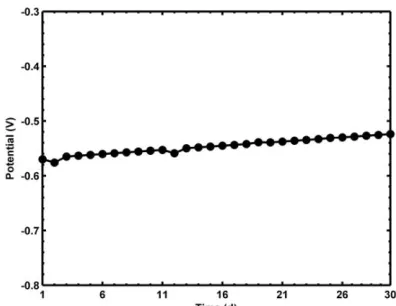
The natural ontology potential V0 between the metal materials and the reference electrodes is illustrated in Figure 3, it shows that V0 is relatively constant. So the polarization potential offset value V2 is obtained by measuring the polarization potential V1.

The characterization parameter V and influence parameters X for the metal material corrosion status are obtained from Metro Line 1 control center in the four traffic intervals, including the polarization potential V1, the rail longitudinal resistance Rt, the rail transition resistance Rg, the railway

voltage U, as shown in Table 1.

Table 1. The data of metal materials corrosion

Traffic Interval X V

l (km) Rt (m) Rg () U (V) V1 (V)

Nanjing → Xinmofan Road 1.685 50.55~64.03 5.93~8.91 -24.9~31.2

-0.993~-0.502 Xinmofan Road →

Xuanwumen

1.060 31.80~40.28 9.43~14.15 -14.7~36.8

-1.691~-0.505 Xuanwumen → Gulou 1.255 37.64~47.67 7.97~11.95

-27.3~35.1

-1.353~-0.501 Gulou → Zhujiang Road 0.863 25.88~32.78 11.59~17.38

-40.4~34.6

-1.265~-0.501

Each traffic interval chose 851 groups of the corrosion samples S, 700 groups for RBF network training, and the remaining 151 groups for the RBF network performance test.

Normalizing S, including X and V

 

 

 

' min

max min

i i

i

i i

s s

s

s s

 

 （15）

Anti-normalizing predictive value Vˆd

 

 

' ˆ

= max min + min( )

i d i i i

V V _ V  V _ V （16）

5.1 RBF neural network based on RPCL and QPSO algorithm

(c) (d)

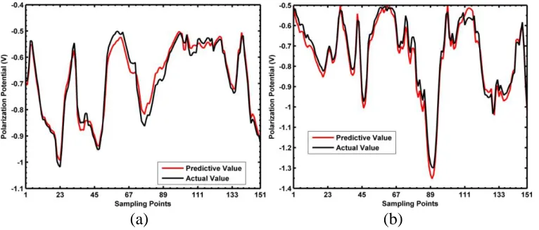
Figure 4. Prediction performance test for Net 1: (a) Nanjing → Xinmofan Road; (b) Xinmofan Road → Xuanwumen; (c) Xuanwumen → Gulou; (d) Gulou → Zhujiang Road

RBF neural network based on RPCL and QPSO algorithm is abbreviated as Net 1, and the hidden layer node number M in Net 1 is obtained using RPCL algorithm. The number k of the initial clustering center {Wj} is 500, the learning ratec and r is 0.03 and 0.01, respectively. The largest clustering times G is 1200, the threshold _minand _max is 1.490 and 1.993, respectively. Therefore, the number M is 73 and the topology of Net 1 is 4×73×1. The particle dimension D is 438, the number of particles R is 50, the maximum generation tmax is 200, and the accuracy eps is 0.0001 in the QPSO

algorithm. Each traffic interval there is 700 groups of corrosion data for Net 1 training, while the remaining 151 groups of corrosion data for Net 1 performance test. The test results are shown in Figure 4.

5.2 RBF neural network based on RPCL algorithm

RBF neural network based on RPCL algorithm is abbreviated as Net 2, and the number M for Net 2 is obtained by RPCL algorithm, while the initial value of the three key parameters are randomly set, namely C,  and W. The prediction performance of Net 2 was compared with that of Net 1, which is used to research the effect of QPSO algorithm on the prediction performance.

(c) (d)

Figure 5. Prediction performance verification for Net 2: (a) Nanjing→Xinmofan Road; (b) Xinmofan Road→Xuanwumen; (c) Xuanwumen→Gulou; (d) Gulou→Zhujiang Road

The parameters k, c , r , G, min and max is 500, 0.03, 0.01, 1200, 1.490 and 1.993, respectively. Similarly, the topology of Net 2 can be identified as 4×73×1. Test the prediction performance of the trained Net 2. The test results are depicted in Figure 5.

5.3 Conventional RBF neural network

(a) (b)

(c) (d)

The conventional RBF neural network is abbreviated as Net 3, which was compared with Net 2 to study the effect of RPCL algorithm on the prediction performance. The hidden layer node number M for Net 2 are randomly set based on experience. Therefore, the topology of Net 3 was set as 4×169×1. The performance test results are shown in Figure 6.

5.4 BP neural network

(a) (b)

(c) (d)

Figure 7. Prediction performance test for BP neural network: (a) Nanjing → Xinmofan Road; (b) Xinmofan Road → Xuanwumen; (c) Xuanwumen → Gulou; (d) Gulou → Zhujiang Road

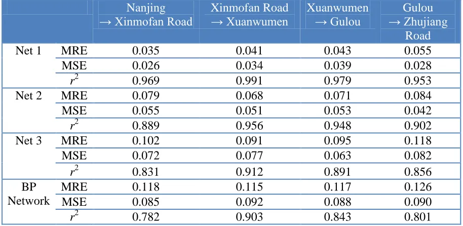
5.5 Prediction performance comparison of the four networks

The mean relative error (MRE) and the mean squared error (MSE), as given by Eq. (17) and Eq. (18), respectively, were both used as the measurement of predictive accuracy. Additionally, the accurate efficiency was measured by the Correlation Coefficient (r2), given by Eq. (19). Note that the values of MSE indicate the deviations between the actual value and predictive value. The larger r2 means the predictive model is more efficient and the maximum value of r2 is one.

1 ˆ 1 MRE m i i i i V V m  V











1 1 _ˆ MSE m i i i V V m 





2

1 1 1

2

2 2

2 2

1 1 1 1

ˆ ˆ

ˆ ˆ

m m m

i i i i

i i i

m m m m

i i i i

i i i i

m V V V V r

m V V m V V

        _        _{ }  _{ }     _{ }  _{ }   _{ }  _{ }    



 









where m is the total number of predictive periods. Vˆ_i and Vi is the predictive and actual value,

respectively.

Table 2. Comparison of prediction performance for the four networks

Nanjing → Xinmofan Road

Xinmofan Road → Xuanwumen Xuanwumen → Gulou Gulou → Zhujiang Road

Net 1 MRE 0.035 0.041 0.043 0.055

MSE 0.026 0.034 0.039 0.028

r2 0.969 0.991 0.979 0.953

Net 2 MRE 0.079 0.068 0.071 0.084

MSE 0.055 0.051 0.053 0.042

r2 0.889 0.956 0.948 0.902

Net 3 MRE 0.102 0.091 0.095 0.118

MSE 0.072 0.077 0.063 0.082

r2 0.831 0.912 0.891 0.856

BP Network

MRE 0.118 0.115 0.117 0.126

MSE 0.085 0.092 0.088 0.090

r2 0.782 0.903 0.843 0.801

the r2 increased by 9.0%. Similarly, it is concluded that the QPSO algorithm can determine the optimal network key parameters, including C,  and W, improving further the prediction performance of the RBF network. Compared with the prediction performance of BP network, the MRE and MSE of RBF network (Net 3) decreased by 15.7% and 18.1 % respectively, while the r2 increased by 5.9%. Therefore, the RBF network is better than the BP network on the corrosion status prediction.

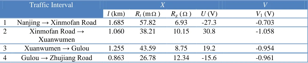
5.6 The practical application of Net 1

During the four traffic interval of Line 1, the metal material corrosion status was predicted using Net 1 in the area without reference electrodes, as shown in Table 3. Referring to Fig. 4, the natural ontology potential is relatively constant, V0 ∈ [-5.760, -0.524]. The natural ontology potential is taken as -0.524 V to facilitate analysis. Therefore, the polarization potential offset values in turn are -0.179 V, -0.534 V, -0.430 V and -0.437 V in the traffic intervals in Table 3. According to the notes on China Standard (CJJ 49 – 1992), the polarization potential offset value has to be limited to a maximum of 0.5 V in metro. Therefore, the metal materials may have been interfered by the stray current, which should be protected in the traffic intervals of 2, 3 and 4.

Table 3. Practical application of Net 1

Traffic Interval X V

l (km) Rt (m) Rg () U (V) V1 (V)

1 Nanjing → Xinmofan Road 1.685 57.82 6.93 -27.3 -0.703

2 Xinmofan Road → Xuanwumen

1.060 38.21 10.15 30.8 -1.058

3 Xuanwumen → Gulou 1.255 43.59 8.75 19.2 -0.954

4 Gulou → Zhujiang Road 0.863 26.78 12.34 -15.6 -0.961

6. CONCLUSIONS

The corrosion status prediction method for the metal materials in the stray current interference was studied in this paper and main results are as follows.

(1) The metro metal material corrosion is classified as the electrochemical corrosion and the corrosion amount of metal materials obeys Faraday's law in the stray current interference. The polarization potential offset values of metal materials characterize the corrosion status, and the polarization potential is directly measured when the natural ontology potential is constant. The traction substation distance l, the rail longitudinal resistance Rt, the rail voltage U and the resistance Rg between

the rails and the metal materials are the key influence parameters of the corrosion status.

which gets the complete RBF network topology. The optimal key parameters are obtained using the QPSO algorithm. Both of these two algorithms can improve the prediction performance of RBF neural network.

ACKNOWLEDGEMENT

This work was supported by Technology Support Project of Jiangsu Province of China under Grant SBE201000378, by Priority Academic Program Development of Jiangsu Higher Education Institutions (PAPD), and in part by Fundamental Research Funds for the Central Universities of China under Grant 2012DXS02.

References

1. L. Bertolini, M. Carsana, P. Pedeferri, Corros. Sci., 49 (2007) 1056-68. 2. K. Zakowski, W. Sokolski, Corros. Sci., 41 (1999) 2099-111.

3. A. L. Cao, Q. J. Zhu, S. T. Zhang, B. R. Hou, Anti-Corros. Method M., 57 (2010) 234-7. 4. F. C. Robles Hernandez, G. Plascencia, K. Koch, Eng. Fail Anal., 16 (2009) 281-94. 5. A. Shamsad, Cement Concrete Comp., 25 (2003) 459-471.

6. S. Srikant, T. S. N. Sankaranarayanan, K. Gopalakrishna, B. R. V. Narasimhan, T. V. K. Das, S. K. Das, Eng. Fail Anal., 12 (2005) 634-51.

7. K. Zakowski, K. Darowicki, Anti-Corros. Method M., 50 (2003) 25-33.

8. C. Andrade, I. Martinez, M. Castellote, J. Appl. Electrochem., 38 (2008) 1467-76. 9. K. Zakowski, Anti-Corros. Method M., 54 (2007) 294-300.

10.K. Darowicki, K. Zakowski, Corros. Sci., 46 (2004) 1061-70. 11.Y. C. Liu, J. F. Chen, IEE P-Elect. Pow. Appl., 152 (2005) 612-8. 12.Y. S. Tzeng, C. H. Lee, IEEE T. Power Deliver., 25 (2010) 1516-25. 13.C. H. Lee, C. J. Lu, IEEE T. Power Deliver., 21 (2006) 1941-7. 14.K. Zakowski, K. Darowicki, Corros. Rev., 19 (2001) 55-67.

15.L. Wei, Stray Current Corrosion Monitoring and Protection Technology in DC Mass Transit Systems, China University of Mining and Technology Press, Xu Zhou (2004).

16.I. A. Metwally, H. M. Al-Mandhari, A. Gastli, Z. Nadir, Eng. Anal. Bound Elem., 31 (2007) 485-93.

17.S. L. Chen, S. C. Hsu, C. T. C. T. Tseng, K. H. Yan, H. Y. Chou, T. M. Too, IEEE T. Veh. Technol., 55 (2006) 67-75.

18.L. I. Frejman, Zashch. Met., 39 (2003) 194-9. 19.D. Paul, IEEE T. Ind. Appl., 38 (2002) 818-24.

20.K. D. Pham, R. S. Thomas, W. E. Stinger, Proceedings of The 2001 IEEE/ASME Joint Railroad Conference, 2001, p. 141-60.

21.K. Zakowski, W. Sokolski, Corros. Sci., 41 (1999) 2213-22. 22.I. Yilmaz, O. Kaynar, Expert Syst. Appl., 38 (2011) 5958-66. 23.J. Wu, J. Liu, Expert Syst. Appl., 39 (2012) 1883-8.

24.H. Han, Q. Chen, J. Qiao, Neural Networks, 24 (2011) 717-25.

25.T. M. Nair, C. L. Zheng, J. L. Fink, R. O. Stuart, M. Gribskov, Comput. Biol. Chem., 27 (2003) 565-74.

26.N. Elfelly, J. Dieulot, M. Benrejeb, P. Borne, Eng. Appl. Artif. Intel., 23 (2010) 1064-71.

27.S. N. Omkar, R. Khandelwal, T. V. S. Ananth, G. Narayana Naik, S. Gopalakrishnan, Expert Syst. Appl., 36 (2009) 11312-22.

28.M. Xi, J. Sun, W. Xu, Appl. Math. Comput., 205 (2008) 751-9.

30.F. J. Pontes, A. P. D. Paiva, P. P. Balestrassi, J. R. Ferreira, M. B. D. Silva, Expert Syst. Appl., 39 (2012) 7776-87.