NATIONAL BANK OF BELGIUM
WORKING PAPERS - RESEARCH SERIES
FORECASTING WITH A BAYESIAN DSGE MODEL:
AN APPLICATION TO THE EURO AREA
_______________________________
Frank Smets(*) Raf Wouters(**)
The views expressed in this paper are those of the authors and do not necessarily reflect the views of the National Bank of Belgium.
This paper was prepared for the 2003 Sveriges Riksbank Workshop on “Small structural models for monetary policy analysis: progress, puzzles and opportunities” and was presented at the 6th European Workshop on “EMU: Current state and future prospects” in Rethymno on 24-31 August 2003. We thank Chris Sims for stimulating comments. The views expressed in this paper are our own and do not necessarily reflect those of the European Central Bank or the National Bank of Belgium.
(*)
European Central Bank, CEPR and University of Ghent, (e-mail: [email protected]). (**)
Editorial Director
Jan Smets, Member of the Board of Directors of the National Bank of Belgium
Statement of purpose:
The purpose of these working papers is to promote the circulation of research results (Research Series) and analytical studies (Documents Series) made within the National Bank of Belgium or presented by outside economists in seminars, conferences and colloquia organised by the Bank. The aim is thereby to provide a platform for discussion. The opinions are strictly those of the authors and do not necessarily reflect the views of the National Bank of Belgium.
The Working Papers are available on the website of the Bank:
http://www.nbb.be
Individual copies are also available on request to:
NATIONAL BANK OF BELGIUM
Documentation Service boulevard de Berlaimont 14 B - 1000 Brussels
Imprint: Responsibility according to the Belgian law: Jean Hilgers, Member of the Board of Directors, National Bank of Belgium. Copyright © National Bank of Belgium
Abstract
In monetary policy strategies geared towards maintaining price stability conditional and
unconditional forecasts of inflation and output play an important role. In this paper we
illustrate how modern sticky-price dynamic stochastic general equilibrium (DSGE) models,
estimated using Bayesian techniques, can become an additional useful tool in the
forecasting kit of central banks. First, we show that the forecasting performance of such
models compares well with a-theoretical vector autoregressions. Moreover, we illustrate
how the posterior distribution of the model can be used to calculate the complete
distribution of the forecast, as well as various inflation risk measures that have been
proposed in the literature. Finally, the structural nature of the model allows computing
forecasts conditional on a policy path. It also allows examining the structural sources of the
forecast errors and their implications for monetary policy. Using those tools, we analyse
macroeconomic developments in the euro area since the start of EMU.
JEL-classification: E4-E5
TABLE OF CONTENTS:
1. INTRODUCTION... 1
2. A BRIEF DESCRIPTION OF THE ESTIMATED EURO AREA MODEL ... 2
2.1 The Smets-Wouters DSGE model ... 2
2.2 Posterior parameter estimates ... 3
3. THE SMETS-WOUTERS MODEL AS A PROJECTION MODEL: SOME ILLUSTRATIONS ... 5
3.1 Out-of-sample forecast performance ... 5
3.2 Forecast uncertainty and confidence bands ... 5
3.3 Measures of risks to price stability ... 6
3.4 Projections under alternative monetary policy scenarios... 7
4. EURO AREA ECONOMIC AND MONETARY POLICY DEVELOPMENTS SINCE 1999... 9
5. CONCLUSIONS... 14
REFERENCES... 15
APPENDIX: THE LINEARISED DSGE MODEL (Smets and Wouters, 2003c) ... 17
1.
Introduction
Due to the lags with which changes in monetary policy affect the economy, projections of inflation
and economic activity play an important role in monetary policy strategies geared towards
maintaining price stability, practised in most industrial countries. At inflation targeting central banks
such as the Bank of England, the Reserve Bank of New Zealand and the Sveriges Riksbank, the
inflation forecast is a central tool for communicating the outlook for price stability and the associated
monetary policy decisions.1 While less prominent, projections of inflation and real GDP also play an
important role at the European Central Bank and the Federal Reserve Board.2 Traditionally, those
forecasts are derived using a combination of relatively large-scale macro-econometric models and a
good deal of judgement.3 As discussed in Sims (2002), the macro-econometric models typically used
at central banks for forecasting are estimated using single-equation methods and often lack a
theoretically consistent model structure and treatment of expectations. While smaller-scale models
with micro-foundations are frequently used for policy analysis, they are not used as forecasting tools
on the basis of the arguments that they are often too simple and perform poorly in forecasting.
In a recent set of papers (Smets and Wouters, 2003a,b), we have shown that modern micro-founded
dynamic stochastic general equilibrium (DSGE) models with sticky prices and wages along the lines
developed by Christiano, Eichenbaum and Evans (2003) are sufficiently rich to capture most of the
statistical features of the main macro-economic time series. Moreover, applying Bayesian estimation
techniques, we show in those papers that even relatively large models can be estimated as a system.
Not only does the system-wide estimation procedure deliver a more efficient estimate of the structural
model parameters, it also provides a consistent estimate of the structural shock processes driving
recent economic developments. Understanding the contribution of the various structural shocks to
recent economic developments is an important input in the monetary policy decision process. Finally,
our recent papers have also demonstrated that the estimated DSGE models perform quite well in
forecasting compared to standard and Bayesian vector autoregressions (VARs and BVARs).
The combination of a sound micro-founded and theoretically consistent model structure and good
forecasting performance suggests that these models could be further developed as an important tool
for both policy analysis and forecasting in central banking. The micro foundations imply that the
structural parameters are more likely to be invariant to various policy interventions the policy makers
may want to consider. As such, one can more easily justify considering projections under different
hypothetical monetary policies using those models.4 The probabilistic nature of the estimated model
implies that those models can also easily be used to assess forecast uncertainty and to perform a
1
See, for example, Bernanke et al (1999). 2
For the role of macro-economic projections in the ECB’s strategy, see, for example, ECB (2001). 3
model and data consistent risk analysis. Since the introduction of the inflation targeting regimes in the
late 1980s and early 1990s, the focus in the assessment of the inflation outlook has shifted from its
central tendency to an analysis of the full forecast distribution and the associated risks.5 The Bayesian
estimation methodology provides an easy-to-use set of tools that can be used to perform such a risk
analysis.
Following our earlier work (Smets and Wouters, 2003a,b), this paper further illustrates how Bayesian
DSGE models can become a useful tool for projection and analysis in central banking. Following a
brief description of the estimated euro area model in Section 2, Section 3 starts with a comparison of
the forecasting performance of the DSGE model with that of VARs and BVARs. We then illustrate
how the empirical posterior distribution of the model can be used to calculate the complete
distribution of the forecast, as well as various risk measures that have been proposed in the literature.
Moreover, we use the model to compute forecasts conditional on a policy path and show how the
outlook for price stability and the associated risks may be affected by alternative monetary policy
scenarios. An important assumption underlying this exercise concerns the response of private sector’s
expectations to changes in the future path of interest rates. In Section 4, we then analyse economic
and monetary policy developments in the euro area since the start of EMU through the lens of the
estimated DSGE model. The structural nature of the estimated model allows us to examine the
structural sources of the forecast errors and their implications for monetary policy. Overall, the
messages that come from this exercise appear to compare well with the policy assessment made by the
ECB over the past years.
2.
A brief description of the estimated euro area model
2.1.
The Smets-Wouters DSGE model
For this paper, we re-estimate the model developed and estimated for the euro area in Smets and
Wouters (2003b,c) over an extended sample period (1980:1-2002:4).6 The DSGE model contains a
large number of nominal and real frictions and various structural shocks. We refer to Smets and
Wouters (2003b) for the detailed derivation. The appendix contains a list of the linearised model
equations.
Households maximise a non-separable utility function in consumption and labour effort over an
infinite life horizon. Consumption appears in the utility function relative to a time-varying external
5
The introduction of fan charts is one example of this shift in focus. See also the discussion in Svensson (2001) on inflation forecast distribution targeting. The importance of risk assessment by central bankers is also underlined in Greenspan (2003).
6
habit variable that depends on past aggregate consumption. Each household provides differentiated
labour inputs. Monopoly power in the labour market results in an explicit wage equation and allows
for the introduction of sticky nominal wages as in the Calvo model (households are allowed to reset
their wage each period with an exogenous probability). Households rent capital services to firms and
decide how much capital to accumulate given certain costs of adjusting the capital stock. The
introduction of variable capital utilisation implies that as the rental price of capital changes, the
capital stock can be used more or less intensively according to some cost schedule. Firms produce
differentiated goods, decide on labour and capital inputs, and set prices according to the Calvo model.
The Calvo model in both wage and price setting is augmented by the assumption that prices that are
not re-optimised in a given period are partially indexed to past inflation rates and the central bank’s
inflation target. Prices are therefore set in function of current and expected marginal costs, but are
also determined by the past inflation rate. The marginal cost of production depends on the wage and
the rental rate of capital. Similarly, wages also depend on past and expected future wages and
inflation.7 Finally, the model is closed with a generalised Taylor rule, where the interest rate is set in
function of the deviation of inflation from a time-varying inflation objective and the theoretically
consistent output-gap (output in deviation from the efficient flexible-price level of output).
The model contains ten identified exogenous driving forces, which are assumed to be orthogonal to
each other. Six of these processes are modelled as autoregressive processes of order one: total factor
productivity, the investment-specific technology process, the intertemporal preference process, the
labour supply process, government spending and the inflation objective of the monetary authorities.
The first five of these exogenous processes are assumed to affect the flexible-price level of output that
enters the central bank’s reaction function as its target level for output. The rationale for this
assumption is that those shocks derive from technology and preferences and should therefore be
accommodated from a welfare perspective. The remaining four shocks are assumed to be white noise:
a price and wage mark-up shock, an equity premium shock and a traditional interest rate (or monetary
policy) shock. Because these shocks are assumed to create inefficient temporary disturbances to the
economy, they do not enter the calculation of the flexible-price output level used in the central bank’s
reaction function. As a result these shocks are more likely to create a trade-off between inflation and
output gap stabilisation.
2.2.
Posterior parameter estimates
As in Smets and Wouters (2003a,b,c), the model is estimated using Bayesian estimation techniques on
seven key macro-economic time series for the euro area: real GDP, consumption, investment,
employment, real wages, inflation in the GDP-deflator and the short run interest rate. These data are
taken from the Area Wide Model database (Fagan et al, 2001) and updated for the most recent period
7
using the ECB Monthly Bulletin. Before estimation, all data are demeaned and the real variables are
linearly detrended.
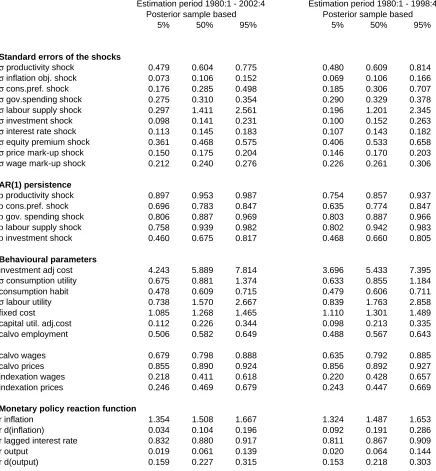
[Insert Table 1]
Table 1 presents the 5, 50 and 95 percentiles of the posterior distribution of the model parameters for
two estimation periods (1980:1-2002:4 and 1980:1-1998:4).8 The latter sample period will be used for
the out-of-sample forecasting exercises performed in Section 3. In this case, the forecast sample starts
with the introduction of the euro in January 1999.
Overall, the estimates seem to be very similar in both samples and broadly in line with our previous
estimates. The total factor productivity and labour supply processes are estimated to be the most
persistent with a median first-order autoregressive coefficient of about 0.95. The three “demand”
shocks have lower persistence.9 As a result, the two “supply” shocks, productivity and labour supply,
will tend to explain most of the forecast error variance for the real variables at the medium to
long-term horizon. The non-stationary inflation objective shock has a relatively high standard error of
0.10%, which corresponds to a change in the inflation objective of 0.4% on a yearly basis. The
estimated inflation target follows a downward trend over the whole estimation sample with an
interruption around 1990. The interest rate shock has a standard error around 0.14% (or 56 basis
points on a yearly basis).
Also the estimates of the behavioural parameters are generally reasonable and close to those estimated
in Smets and Wouters (2003a,c). As in our previous paper, the Calvo parameter for price setting
(0.89) implies a very high degree of price stickiness with prices on average remaining fixed for more
than two years. Nevertheless, our estimate of the elasticity of inflation with respect to the marginal
cost is very similar to those obtained by Gali, Gertler and Lopez-Salido (2001). The results for the
hypothetical historical policy rule are relatively standard. The long run reaction on inflation is exactly
equal to the one assumed in the original Taylor rule (1.5). The long run reaction coefficient on the
output-gap is smaller than in the prototype Taylor rule (0.2). The policy reaction function exhibits a
high degree of persistence with a coefficient on the lagged interest rate of 0.88. While
policy-controlled interest rates do not react strongly to the level of the output gap, they do to changes in the
output gap. The reaction coefficient to current changes in inflation is somewhat higher in the shorter
sample, indicating that the recent mild reaction to the price mark-up shocks has lowered this
parameter estimate.
8
The data from 1970:2 till 1979:4 were used to evaluate the unobserved state variables, so that the starting values at time 1980:1 are based on these historical realisations.
9
3.
The Smets-Wouters model as a projection model: some illustrations.
3.1.
Out-of-sample forecast performance
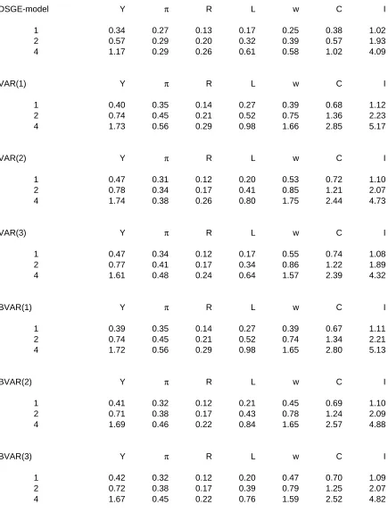
To illustrate the good prediction performance of the DSGE model, in this Section we perform a
traditional out-of-sample prediction exercise over the post-EMU period 1999:1 - 2002:4. As the
forecasting period is relatively short, these results are only indicative. We compare the root mean
squared errors (RMSEs) of the forecasts from the DSGE model with those from standard VARs and
BVARS of order 1 to 3 in Table 2. Starting from the pre-EMU sample, the VAR and BVAR models
are re-estimated quarterly, while the DSGE model is re-estimated only yearly. Given the relatively
short sample, Table 2 reports the RMSEs for horizons of 1 to 4 quarters only.
[Insert Table 2]
Overall, this exercise confirms the good forecasting performance of the DSGE model, highlighted in
Smets and Wouters (2003a,b). The RMSEs are quite a bit lower than those obtained for the VAR
models. This is true for each of the macro-economic time series (with the partial exception of the
nominal interest rate) and at all horizons considered. Moreover, there is some evidence that the
forecast performance improves as the horizon lengthens.
3.2.
Forecast uncertainty and confidence bands
As discussed in the introduction, the Bayesian estimation methodology provides a useful set of tools
for calculating the full probability distribution around the central forecast. Graph 1 illustrates the
uncertainty surrounding the projections of each of the seven macro-economic variables at the
beginning of 1999. A comparison of the actual time series with the 5-95 percentile forecast interval
suggests that there is no clear evidence of instability in the estimated model following the introduction
of the euro in 1999. The bounds appear to be realistic measures of the forecast uncertainty in the
sense that there are only a few exceptions in which actual developments touch the 5% tails of the
forecast distribution.
[Insert Graph 1]
The calculation of the forecast bounds in Graph 1 takes into account that, for a given model, there are
typically two sources of forecast uncertainty: the uncertainty coming from unexpected future shocks
and the uncertainty associated with the parameters of the model. Both sources of uncertainty typically
contribute to large uncertainty bounds around standard VAR-based forecasts. Due to the relatively
tight parameterisation of our estimated DSGE model, the main source of forecast uncertainty as
illustrated in Graph 1 comes from the shock uncertainty. Indeed, the forecast distribution generated by
the estimated parameter uncertainty is very limited. While the highly restricted DSGE model strongly
underestimation of the degree of uncertainty. It is likely that the parameter uncertainty is partly
replaced by model uncertainty, which could only be assessed by estimating alternative theoretical
models and evaluating their influence on the forecast.10
3.3.
Measures of risks to price stability
While the inflation forecast uncertainty can be summarised in fan charts, as, for example, produced by
the Bank of England and the Sveriges Riksbank in their Inflation Reports, such forecast distributions
are often quite difficult to interpret. In a recent paper, Kilian and Manganelli (2003) propose simple
risk measures that quantify the relative uncertainty in the forecasts produced by a statistical model. In
their view, central bankers can be regarded as risk managers who aim at containing inflation within
specified bounds. They develop simple formal tools that are useful to quantify and forecast the risks
that central bankers will fail to obtain the stated objectives. Kilian and Manganelli (2003) propose the
following measures to summarise the risks that inflation will move outside pre-specified bounds. 11
(1)
EIR
t=Prob(π
t+1>π
u)*E[
(
π
t+1−
π
u)
βπ
t+1>π
u]
(2)
DR
t=−Prob(π
t+1<π
l)*E[
(
π
l−
π
t+1)
βπ
t+1<π
l]
The first measure is a measure of excess inflation risk. It is the expected inflation for next period in
excess of an upper bound where the power reflects the relative risk aversion in the central bankers’
preferences multiplied by the probability (prob) that the inflation realisation is above the limit. The
second measure is a measure of deflation risk. In line with the ECB’s definition of price stability, we calculate these measures for an upper bound (πu) of 2% and a lower bound (πl) of 0% for the
average inflation rate over the next four quarters12. In line with Kilian and Manganelli (2003) and
most of the literature on optimal monetary policy, we assume a coefficient of risk aversion (β) equal
to two. The sum of the projected excess inflation and deflation risk measures can be seen as a
measure of the projected one-year ahead balance of risks to price stability:
(3)
BR
t=
EIR
t+
DR
tThe posterior distribution of the DSGE model can easily be used to calculate the risk measure
proposed by Kilian and Manganelli (2003). Graph 4, which will be discussed in detail in section 4,
illustrates the development of those risk measures since the start of EMU. For example, at the start of
1999 the balance of inflation risks dropped quite considerably following the fall-out from the Russian
10
See, for example, the discussion in Brock, Durlauf and West (2003) and Sims (2003). 11
As the fan charts in the Inflation Reports of the Bank of England and the Sveriges Riksbank are not based on statistically generated distribution functions, but rather reflect the subjective uncertainty around the inflation and output forecasts of the policy makers, it is much more difficult to calculate such risk measures based on the fan charts.
12
crisis. In section 4 we will use these measures to interpret economic and monetary policy
developments in the euro area since 1998.
3.4.
Projections under alternative monetary policy scenarios
The projection exercises presented in the previous sections were performed under the assumption that
the European Central Bank followed the interest rate reaction function estimated over the pre-EMU
period. Often such projections are called unconditional forecasts. Typically, however, monetary
policy makers prefer to use constant nominal-interest-rate forecasts.13 Such conditional projections
provide a natural benchmark for assessing whether interest rates need to be changed given the central
bank’s goal of maintaining price stability. They also avoid the need to specify the central bank’s
reaction function, which may not be very easy to do in particular following a regime change such as
the introduction of the euro. However, producing such conditional projections using rational
expectations models raises two issues. First, it is well known that rational expectations models will
typically not solve under a constant nominal interest rate path because nominal interest rate pegging
often leads to an explosive path for the ex-ante real interest rate, output and inflation. One solution to
this problem is to assume that the nominal interest rate is kept constant for a limited period of time,
say three years, after which a policy reaction function kicks in putting the economy again on an
equilibrium path.
A second issue raised by a constant interest rate projection concerns how to implement the constant
interest rate path in a forward-looking model. At least two options are available. One option, applied
in this section, is to calculate the monetary policy shocks that are necessary to keep the interest rate on
a constant path relative to the historically estimated reaction function. The advantage of this option is
that current economic variables that depend on expectations of future interest rates (such as various
asset prices, but also consumption and investment) will only gradually respond to the constant interest
rate scenario. This option is also closest to the analysis of modest policy interventions using Bayesian
VARs in Leeper and Zha (2003)14. Of course, as emphasised by Leeper and Zha (2003), this
assumption only makes sense if the required unexpected policy shocks are relatively small and
comparable in size to the historically estimated policy shocks. A second option is to assume that the
private sector has perfect foresight of the constant interest rate path and adjusts its decisions in line
with this change in expected policy. This approach is fully compatible with the rational expectations
assumption embedded in our estimated DSGE model. However, it will typically lead to relatively
large jumps in all the forward-looking variables including consumption and investment, which in
some circumstances may be perceived as implausible.
13
Also at the European Central Bank the macro-economic projection of the Eurosystem staff are based on the assumption of constant nominal short-term interest rates.
14
[Insert Graph 2]
Graph 2 plots the forecast distribution of the seven macroeconomic variables at the end of 1998
(similar to Graph 1) under the assumption that the nominal interest rate is kept constant for three
consecutive years (after which the estimated reaction function kicks in). The private sector continues
to think that the central bank follows the estimated reaction function and treats the deviations of
actual interest rates from the expected interest rates as policy shocks. The graph shows that because
the monetary authorities keep nominal interest rates persistently below their expected path (see Graph
1), the median forecast for output and inflation is much higher than projected in Graph 1. It is also
clear from comparing Graphs 1 and 2 that the uncertainty surrounding the median forecast is much
higher under the constant interest rate path. As monetary policy is passive the effects of future shocks
are projected to be much larger.
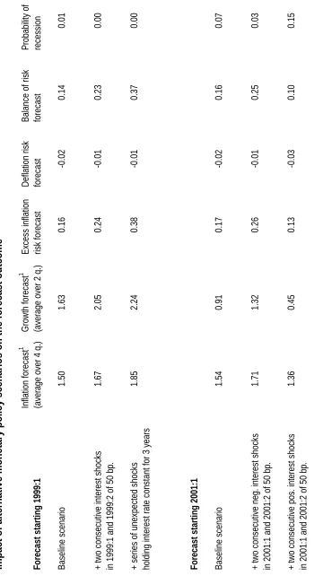
Table 3 summarises the effects of the constant interest rate assumption on the inflation and output
growth forecast and the various risk measures at two points in time: 1998:4 and 2000:4. These two
dates correspond to the start of the two sub-periods that will be discussed below in Section 4. In
1998:4, the unconditional median forecast for inflation over the next year and growth over the next
two quarters was 1.5 percent and 1.63 percent respectively. According to this forecast, the balance of
inflation risks was slightly tilted upwards and the probability of a recession (defined as two
consecutive quarters of negative growth) was negligible at 0.01. Under this scenario, short-term
interest rates were expected to increase gradually to their long-run neutral level of about 5.5%. The
third line in Table 3 shows the impact of a constant interest rate path for three years. The inflation and
growth projection increase by respectively 0.35 and 0.61% compared to the baseline scenario. The
excess inflation risk increases reflecting the increase in uncertainty, and the balance of risks also
clearly increases suggesting that upward inflation risks would have dominated under this scenario.
The series of unexpected shocks that are necessary to keep the interest rate path constant for three
years starting in 1998:4 are negative and growing over the three-year period. As such, they can not be
catalogued as a modest intervention.15
[Insert Table 3]
The effects of an alternative and more realistic scenario, in which the interest rate is decreased by 50
basis points for two consecutive quarters starting in 1999:1 (compared to the baseline scenario) is
given in the second line of Table 3. In this case, the median inflation forecast increases with 0.17
percentage points and the growth rate is revised upward by 0.42 percentage points. Also in this case,
the balance of inflation risks would have shifted upward. As discussed below in Section 4, the euro
area faced significant negative demand shocks in the first two quarters of 1999 (partly following the
fall-out of the Russian crisis in 1998) shifting the balance of inflation risks downward. Scenarios such
as the one reported in the second line of Table 3 may be quite informative about the policy choices
15
that policymakers where faced with at the time. The actual decline in the interest rate that occurred in
April 1999 can be partly seen as an attempt to restore the balance of risks.
The lower part of Table 3 performs a similar exercise around the baseline unconditional forecast of
inflation and growth in 2000:4. At that time, the outlook for inflation over the next year and the
associated risks were very similar to the outlook at the beginning of 1999. However, the outlook for
output growth was less favourable with a 7 percent probability of a recession. The bottom two lines of
Table 3 illustrate the effect of two alternative scenarios: a reduction and an increase in interest rates
of 100 basis points in total. A reduction in interest rates would have supported growth considerably
reducing the probability of a recession, but at a cost of increased inflation by about 17 percentage
points. In contrast, the interest rate increase would have increased the probability of a recession quite
considerably to 15%.
The exercises performed in this section illustrate the potential usefulness of our Bayesian DSGE
model in assessing the impact of alternative monetary policy scenarios on the outlook for price
stability and the associated risks. It is, however, important to re-emphasise that the reported results
crucially depend on the assumptions made about how expectations of private agents adjust to the
alternative interest rate paths. In the exercises reported above, we implemented alternative interest
rate paths by shocking the estimated interest rate reaction function. As discussed in Leeper and Zha
(2003), this makes sense if the shocks are relatively modest. However, identical interest rate paths
could also be implemented under the assumption of perfect foresight or with alternative systematic
monetary policy reaction functions and their associated shocks. The impact of these alternative
assumptions may very well be non-negligible. This is an important question for future research.
4.
Euro area economic and monetary policy developments since 1999
One advantage of the structural nature of the estimated DSGE model is that the model can be used to
analyse the structural sources of the shocks that have affected the euro area economy during the first
four years of EMU. As is clear from Graph 1, the first four years of EMU (1999:1-2002:4) can be
roughly divided into two equal sub-periods. The first sub-period (1999:1-2000:4) was characterised
by relatively strong output, employment and real wage growth. In contrast, the second sub-period
(2001:1-2002:4) is characterised by a slowdown in economic activity, a stabilisation of real wages and
a temporary surge in inflation. In what follows, we interpret each of those periods through the lens of
the estimated DSGE model.
The first two years of EMU
Graph 1 shows that, at the end of 1998, the baseline projection as captured by the median forecast of
our model was for the economy to gradually return to its deterministic growth path following a
slightly negative output gap at the end of 199816. As a result, the model predicts as a median scenario
16
relatively stable growth of the economy, with a slightly above average growth for investment and
employment in the first years of the forecast exercise. Inflation is expected to increase slightly
towards the implicit inflation target of monetary policy that is estimated to be somewhat below 2 % at
the end of 1998. As part of this move to equilibrium, the nominal interest rate is forecast to return
relatively quickly to its equilibrium level.
Graph 1 also shows that by the end of 2000, most of the actual time series were close to their
projected values. One exception is employment, which grew much stronger than expected. Moreover,
this end-of-2000 snapshot masks some volatility in economic developments during the first two years
of EMU. Graph 3 presents the estimated structural shocks during this period together with a
one-standard-error band. Graphs 4 and 5 show the resulting evolution of the balance of inflation risks and
its components over the period.
[Insert Graph 3]
Starting from a slightly positive balance of risks in the fourth quarter of 1998, our estimated model
suggests that deflation risks rose while excess inflation risks fell during the first half of 1999 (Graph
4). As a result, the risks were quite balanced in the second quarter of 1999. This is mainly a result of
the negative spending shock in the first quarter of 1999 (mostly reflecting a fall in the demand for net
exports following the fall-out from the Russian financial crisis at the end of 1998) and the subsequent
negative preference shock in the second quarter of 1999. As a result, in contrast to what was forecast
by the model, nominal interest rates fell during the first half of 1999. However, the interest rate
appears to have fallen by more than predicted by the estimated policy reaction function, thereby
supporting output and investment in the following year. Subsequently, deflation risks fell, while
excess inflation risks rose towards the end of 1999 and in 2000. This led to a reversal and gradual rise
in policy-controlled interest rates, which approach the forecast level towards the end of 2000. The
most striking development in the first sub-period is the stronger than expected development of
employment, which contributed to a stabilisation of real wages in the second half of 2000. The
positive effects on output are, however, partly offset by a series of negative productivity shocks over
the same period17.
[Insert Graph 4]
A reading of the Editorials of the ECB’s Monthly Bulletin suggests that the changing balance of risks
as captured by our model in the first two-years of EMU more or less corresponds to the ECB’s
interpretation of events. In the beginning of 1999, HICP inflation was lower than previously expected
and was explained by subdued growth of unit labour costs in 1998 and by the downward risk
following the Asian crisis. The March 1999 Monthly Bulletin read: "In the light of recent
developments in real economy indicators, and taking into account the current level of HICP inflation
17
rates, it appears that there is no risk of HICP inflation exceeding the 2% ceiling in the near future. At
the same time, the pattern of upward and downward risks to price stability has remained broadly
unchanged on balance." The reduction of official interest rates from 3% to 2.5% in April 1999, was
motivated in the April 1999 Monthly Bulletin by increased downward inflation risks: "This picture is
also reflected in recent downward revisions to real GDP forecasts for the euro area in 1999 and 2000
by major international organisations. ... the downward revisions in the growth forecasts and
uncertainty concerning these forecasts have reinforced expectations of somewhat lower inflationary
pressure arising from economic activity this year."
Also the favourable developments in the labour market were clearly identified as unexpected surprises
in the following quote from the September 2000 Monthly Bulletin. "Euro area employment growth
has recently been revised upwards, in particular for the past two years, and is now estimated to have
reached a remarkable annual rate of growth of close to 2% in the first half of 2000. This dynamism
reflects robust economic growth and wage moderation, and may also point to some progress in
labour market flexibility. Continued moderate wage increases would contribute to maintaining the
favourable trends in labour market developments in the context of still high unemployment."
However, the fall in total factor productivity identified by our model was not commented upon.
Finally, the series of interest rate increases that started in December 1999 and continued during the
course of 2000 were largely based on a rise in the upward risks to price stability due to strong output
and employment growth in a favourable international environment and the delayed pass-through of
the depreciation of the euro and the rise in energy prices. Due to the use of the GDP deflator rather
than the HICP, these cost-push shocks only show up with a delay in our model’s forecasts.18 For
instance, in the April 2000 Monthly Bulletin, the official interest increase from 3.25% to 3.5% dated
17 March was commented upon as follows: "This picture of continuing strong domestic demand
supports the favourable outlook for economic growth in the euro area as shown in recent forecasts.
The positive prospects for euro area activity are also benefiting from the cyclical upswing in the
world economy, which has become broadly based across industrial and emerging economies and
which is expected to continue in coming years. ... Against this background, monetary policy must
remain vigilant in assessing upside risks to price stability and take appropriate action if and when
18
required. Monetary policy has to be forward-looking, since responding to risks to price stability
before they materialise will avoid the need for costly process of disinflation at a later stage."
Less favourable developments than projected during the 2001 - 2002 period
Graph 5 depicts the forecast distribution based on information up to the fourth quarter of 2000 for the
seven euro area macro variables in 2001 and 2002. The estimated DSGE model predicted a more
modest growth of consumption, investment and output than realised growth in 2000. Employment was
projected to remain constant and wages were projected to increase relatively strongly as the model
expected the favourable labour supply shocks over the first two years of EMU to gradually die out
over time. Inflation and the nominal interest rate were predicted to gradually return to their long run
levels corresponding to a 1.5% inflation objective (estimate at 2000:4) and a 5.5% equilibrium
nominal interest rate respectively.
With the exception of the labour market developments, the actual outcome in 2001 and 2002 was
much less rosy than projected. Real GDP and particularly real investment turned out much lower than
expected due to a series of negative investment technology, equity premium and productivity shocks
(Graph 3). The impact of the drop in investment on output is somewhat offset by the mostly positive
labour supply shocks over this period. In the last quarter of 2001, the negative shocks to investment
are reinforced by a large negative preference shock reflecting the confidence effects of the September
11 attacks in the US on consumption. Also on the inflation side the news was predominantly negative
as a series of positive price mark-up shocks pushed inflation above the projected level in spite of the
favourable developments in real wages.
[Insert Graph 5]
The implications of the various shocks in 2001 and 2002 for the evolution of the one-year ahead
projected inflation and the balance of inflation risks is again shown in Graphs 4 and 5. Despite the
large positive mark-up shocks which reflect the effects of the depreciation of the euro and rising food
and energy prices on inflation, the balance of risks rapidly dropped from its maximum in the first
quarter of 2001 to a negative value in the third quarter of 2001, indicating the dominance of
downward risks to price stability. The model sees through the temporary effects of the mark-up
shocks and puts a dominant weight on the negative demand shocks when assessing the risks to price
stability. Following a brief surge in the excess inflation risks due to a new series of price mark-up
shocks, the downward risks clearly dominate during most of 2002. This occurred in spite of the fact
that the easing of monetary policy appeared to be stronger than could be expected on the basis of the
hypothetical historical reaction function as indicated by the negative monetary policy shocks
throughout most of 2001 and 2002 (Graph 3).19 In the second half of 2002 the probability of one-year
ahead deflation is estimated to be relatively high at around 25%.
19
The picture drawn by the one-year ahead balance of risks indicator produced by our model again
corresponds quite closely with the discussion in the ECB’s Monthly Bulletins. The first sign of
increased concern about the international environment appeared in the December 2000 Monthly
Bulletin coinciding with the slight drop in our excess inflation risk indicator during the last quarter of
2000. While in January 2001 the risks to price stability were still predominantly seen on the upside, in
February and even more clearly in March, the risks appeared to be evaluated as more balanced than in
late 2000, although it was also stated that there were not yet signs that the slowdown in the US
economy had significant or lasting spill-over effects on the euro area. In the April 2001 Monthly
Bulletin the balance clearly tilted to the downside. This foreshadowed the policy easing that was in
the pipeline and eventually happened on 10 May, mainly based on the risk analysis rather than on
observed data. During this period the ECB expressed a clear satisfaction with the maintained wage
moderation that has supported employment growth, while repeatedly warning for possible spill-over
effects from the price shocks.
In the July 2001 Monthly Bulletin, there was a first clear recognition that growth was lower than
expected: "The first Eurostat estimate of real GDP growth in the first quarter of 2001 was 0.5%, as
compared with the 0.6% in the last quarter of 2000. The slowdown appears to be related to the
external environment and to the weak growth of domestic demand. The significant decline in the
growth rate of domestic demand was stronger than expected, with investment being affected both by
the adverse influences from the world economy and by specific domestic developments related to
construction investment. At the same time, growth in consumption was weak, which may in part be
explained by adverse income effects relating to the increases in energy and food prices." At the same
time HICP inflation rose to 3.4% in May following the increase in food and energy prices. However,
the ECB stressed that due to the special nature of these shocks, they were likely to only have a
temporary effect on inflation.
Also in the August 2001 Bulletin the lower than expected growth rate was emphasised, eventually
leading to further interest rate easing. In the November issue the November 8 decline in the
policy-controlled interest from 3.75 to 3.25% was motivated as follows: "Several economic indicators which
have become available for the euro area and beyond point to weakening demand of both domestic and
external origin. In line with this and taking into account expectations of further weak data in the
period ahead, forecasts and projections will in all likelihood show downward revisions. The current
environment of high uncertainty is likely to lead to delays in investment and, to some extent, also to
negatively affect private consumption in the euro area. This has led to expectations of weak data for
the euro area real GDP growth in the second half of 2001. Real GDP growth is now expected to
remain below potential for part of next year."
In sum, our stylised estimated DSGE model seems to perform relatively well in capturing the
evolution of the perceived risks to price stability. At the same time, it allows for a structural
5.
Conclusions
Modern sticky-price DSGE models of the type used in this paper and estimated using Bayesian
techniques combine a sound, micro-founded structure necessary for policy analysis with a good
probabilistic description of the observed data and forecasting performance. In this paper we illustrated
how such Bayesian DSGE models can become an additional useful tool in the forecasting kit of
central banks. First, we show that the forecasting performance of such models compares well with
a-theoretical vector autoregressions. Moreover, we illustrate how the posterior distribution of the model
can be used to calculate the complete distribution of the forecast, as well as various inflation risk
measures that have been proposed in the literature. Finally, the structural nature of the model allows
computing forecasts conditional on a policy path. It also allows examining the structural sources of
the forecast errors and their implications for monetary policy. Using those tools, we briefly analysed
and interpreted macroeconomic developments in the euro area since the start of EMU.
Of course, many challenges still lie ahead. Here it suffices to highlight three of those challenges. First,
the structure of the model remains relatively simple and in many cases the micro-foundations are not
very deep. Much more work is needed to both deepen and broaden the scope of the existing DSGE
models. For example, the introduction of more realistic financial and labour markets is one vibrant
area of current research. For practical forecasting exercises, the introduction of an open economy
dimension and the HICP-inflation in addition to the inflation in the GDP-deflator might allow for a
better identification of external demand and price shocks. Second, the assumption of model
consistent expectations is theoretically appealing and relatively easy to implement. However, in
reality constraints on information processing, pervasive model uncertainty and the associated need for
perpetual learning highlight the limits of the rational expectations assumption. When forecasting in a
policy context, realistic assumptions about how private sector expectations will adjust to alternative
policy scenarios are of crucial importance. Finally, the linearity of the model used in this paper is an
attractive feature from a computational and estimation point of view. Linear models are typically also
more robust in forecasting. However, non-linearities due to shifting economic relationships,
time-variation in the sources of shocks, various institutional and technical constraints and the
non-monotone adjustment of expectations are important factors in the risk analysis of monetary policy
makers. While it would be impossible to take into account all those sources of non-linearities in one
model, an analysis of the implications of each of them is an important area of current and future
References
Bernanke, B., T. Laubach, F. Mishkin and A. Posen (1999). Inflation targeting: Lessons from the
international experience. Princeton University Press, Princeton NJ.
Brock, W., S. Durlauf, K. West (2003), “Policy evaluation in uncertain economic environments”,
Brookings Papers on Economic Activity, 2003:2.
Christiano, L., M. Eichenbaum and C. Evans (2003), “Nominal rigidities and the dynamic effects of a
shock to monetary policy”, Journal of Political Economy, forthcoming.
Cogley, T., S. Morozov and T.J. Sargent (2003), "Bayesian fan charts for U.K. inflation: Forecasting
and sources of uncertainty in an evolving monetary system", mimeo.
European Central Bank (2001), “A guide to Eurosystem staff macroeconomic projection exercises”,
European Central Bank, Frankfurt.
Fagan, G., J. Henry and R. Mestre (2001), “An Area-Wide Model (AWM) for the euro area”,
European Central Bank Working Paper 42.
Gali, J., M. Gertler and D. Lopez-Salido (2001), “European inflation dynamics”, European Economic
Review, 45(7), 1121-1150.
Greenspan, A. (2003), Monetary policy under uncertainty, Remarks at a symposium sponsored by the
Federal Reserve Bank of Kansas City, Jackson Hole, Wyoming, 29 August 2003.
Kilian, L. and S. Manganelli (2003), “The central bank as a risk manager: Quantifying and measuring
inflation risks”, European Central Bank Working Paper, April 2003.
Leeper, E. and T. Zha (2003), “Modest policy interventions”, Journal of Monetary Economics, Vol.
50, pp. 1673-1700.
Pagan, A. (2003). “Report on modelling and forecasting at the Bank of England”, Bank of England,
London.
Peersman, G. (2004), "What caused the early millennium slowdown? Evidence based on vector
autoregressions", Journal of Applied Econometrics (forthcoming)
Sims, C. (2002), “The role of models and probabilities in the monetary policy process”, Brooking
Papers on Economic Activity, 2002:2, 1-62.
Sims, C. (2003), “Probability models for monetary policy decisions”, work in progress, Princeton
University.
Smets, F. and R. Wouters (2003a), “An estimated dynamic stochastic general equilibrium model of
Smets, F. and R. Wouters (2003b), “Shocks and frictions in US business cycles: a Bayesian DSGE
approach”, mimeo, European Central Bank.
Smets, F. and R. Wouters (2003c), “Comparing shocks and frictions in US and euro business cycles: a
Bayesian DSGE approach”, forthcoming in Journal of Applied Econometrics
Svensson, L. (2001), “Price stability as a target for monetary policy: defining and maintaining price
stability”, in Deutsche Bundesbank (ed.), The monetary transmission process: Recent developments
Appendix: The linearised DSGE model (Smets and Wouters, 2003c).
The consumption equation:
(1)
) ˆ ( ) 1 ( 1 ) ˆ ˆ ( ) 1 ( 1 ) ( ) 1 )( 1 ( ) 1 ( ˆ 1 1 ˆ 1 ˆ 1 1 11
ˆ
ˆ
b t c t t t c t t w c c t t t t h h E R h h h C E h C h h
C
l
l
ε σ π σ σ σ
λ
+ − + − + − − − + + − + + + + = + + + −Consumption
C
ˆ
t depends on a weighted average of past and expected future consumption, the ex-antereal interest rate
(
R
ˆ
t−
E
tπ
ˆ
t+1)
,
expected employment growth (lˆt+1−lˆt) and a preference shock b tεˆ . h
represents the habit formation coefficient and
σ
cis the analogue of the intertemporal elasticity ofsubstitution.
The investment equation:
(2) (Qˆ ˆ )
1 / 1 Iˆ E 1 Iˆ 1 1
Iˆt t 1 t t 1 β t εtI
ϕ β
β
β + + + + +
+
= − +
Investment Iˆ depends on past and expected future investment, the value of the existing capital stock t
t
Qˆ and an investment-specific technology process,
ε
ˆ
tI. β is the rate of time preference and ϕ is theparameter that summarises the investment adjustment costs.
The Q equation :
(3) t tk tQ
k k t t k t t
t
E
r
r
r
Q
E
r
R
Q
η
τ
τ
τ
π
+
+
−
+
+
−
−
+
−
−
=
+ +ˆ
+1
ˆ
1
1
)
ˆ
ˆ
(
ˆ
1 1 1The value of the capital stock depends negatively on the ex-ante real interest rate, and positively on its
expected future value, the expected rental rate rˆtk+1 and an equity premium shock Q t
η .
The capital accumulation equation:
(4) Kˆt =(1−τ )Kˆt−1+τIˆt−1+τεˆtI−1
The capital stock Kˆt depreciates with a rate τ.
The inflation equation:
(5)
[
]
pt a t t k t p p p p t t p p t t p t t t w r t
E
η γ α ε α α ξ ξ βξ βγ βγ γ βγ βπ
π
π
π
π
π
+ − − − − + − − + + − + + − + = − − + ) 1 ( ˆ ˆ ) 1 ( ˆ ) 1 )( 1 ( 1 1 ) ( 1 ) (1
ˆ
ˆ
ˆ
1 1The deviation of inflation
π
ˆ
t from the target inflation rateπ
t depends on past and expected futureinflation deviations and on the current marginal cost, which itself is a function of the rental rate on
in the marginal cost. (1-ξp) is the probability that prices can be reset in a given period, while γpis
the degree of indexation of prices on past inflation. ηtpis the i.i.d. shock in the price mark-up.
The real wage equation:
(6) w
t L t t t t L t w w L w w w t t w t t w t t t t t t C h C h L w t w w E w
E
η ε σ ξ ξ βξ β β γ β βγ β β β β βλ
σ
λ
π
π
π
π
π
π
+ − + − − − + + − − + − − + + − + + − − + + + + + = − − + − + ˆ ) ˆ ˆ ( 1 1 ˆ ˆ ) ) 1 ( 1 ( ) 1 )( 1 ( 1 1 ) ( 1 ) ( 1 1 ) 1 ˆ 1 1 ˆ 1 ˆ 1 1 1 11
(
ˆ
ˆ
ˆ
The real wage wˆt is a function of expected and past real wages, the expected, current and past inflation rate and the deviation of the actual real wage from the wage that would prevail in a flexible
labour market. ηtwis the i.i.d. shock in the wage mark-up while L t ˆ
ε is the persistent labour supply
shock.
The labour demand equation:
(7)
L
ˆ
t=
−
w
ˆ
t+
(
1
+
ψ
)
r
ˆ
tk+
K
ˆ
t−1Labour demand Lˆt depends negatively on the real wage (with a unit elasticity) and positively on the
rental rate of capital and last period’s capital stock. ψ reflects the capital utilisation adjustment cost.
The goods market equilibrium condition:
(8) t t L r K g I k C g k Y t k t t a t G t y t y t y y t γ φ γ α φ φαψ φα ε φ ε τ τ ) 1 ( ) ˆ )( 1 ( ˆ ˆ ˆ ˆ ˆ ) 1 ( ˆ
1+ + − + − −
+ = + + − − = −
with
k
ythe capital-output ratio and gy the share of public consumption in output. φ reflects the fixedcosts in the production function.
The monetary policy reaction function:
(9)
[
]
[
]
Rt p t t p t t y t t t t p t t Y t t t t t t Y Y Y Y r r Y Y r r R R η π π π π π π ρ π ρ π π π + − − − + − − − + − + − − + − + = − − ∆ − − ∆ − − − − − − ) ) ˆ ˆ ( ) ˆ ˆ ( ) ˆ ( ) ˆ ( )} ˆ ˆ ( ) ˆ ( ){ 1 ( ) ˆ ( ˆ 1 1 1 1 1 1 1 1 1 1
The interest rate Rˆt reacts persistently, via the parameter ρ, on both the level and the first difference
Table 1:
Posterior distribution of the model parameters
Estimation period 1980:1 - 2002:4 Estimation period 1980:1 - 1998:4 Posterior sample based Posterior sample based
5% 50% 95% 5% 50% 95%
Standard errors of the shocks
σ productivity shock 0.479 0.604 0.775 0.480 0.609 0.814
σ inflation obj. shock 0.073 0.106 0.152 0.069 0.106 0.166
σ cons.pref. shock 0.176 0.285 0.498 0.185 0.306 0.707
σ gov.spending shock 0.275 0.310 0.354 0.290 0.329 0.378
σ labour supply shock 0.297 1.411 2.561 0.196 1.201 2.345
σ investment shock 0.098 0.141 0.231 0.100 0.152 0.263
σ interest rate shock 0.113 0.145 0.183 0.107 0.143 0.182
σ equity premium shock 0.361 0.468 0.575 0.406 0.533 0.658
σ price mark-up shock 0.150 0.175 0.204 0.146 0.170 0.203
σ wage mark-up shock 0.212 0.240 0.276 0.226 0.261 0.306
AR(1) persistence
ρ productivity shock 0.897 0.953 0.987 0.754 0.857 0.937
ρ cons.pref. shock 0.696 0.783 0.847 0.635 0.774 0.847
ρ gov. spending shock 0.806 0.887 0.969 0.803 0.887 0.966
ρ labour supply shock 0.758 0.939 0.982 0.802 0.942 0.983
ρ investment shock 0.460 0.675 0.817 0.468 0.660 0.805
Behavioural parameters
investment adj cost 4.243 5.889 7.814 3.696 5.433 7.395
σ consumption utility 0.675 0.881 1.374 0.633 0.855 1.184
consumption habit 0.478 0.609 0.715 0.479 0.606 0.711
σ labour utility 0.738 1.570 2.667 0.839 1.763 2.858
fixed cost 1.085 1.268 1.465 1.110 1.301 1.489
capital util. adj.cost 0.112 0.226 0.344 0.098 0.213 0.335
calvo employment 0.506 0.582 0.649 0.488 0.567 0.643
calvo wages 0.679 0.798 0.888 0.635 0.792 0.885
calvo prices 0.855 0.890 0.924 0.856 0.892 0.927
indexation wages 0.218 0.411 0.618 0.220 0.428 0.657
indexation prices 0.246 0.469 0.679 0.243 0.447 0.669
Monetary policy reaction function
r inflation 1.354 1.508 1.667 1.324 1.487 1.653
r d(inflation) 0.034 0.104 0.196 0.092 0.191 0.286
r lagged interest rate 0.832 0.880 0.917 0.811 0.867 0.909
r output 0.019 0.061 0.139 0.020 0.064 0.144
Table 2:
Comparing out-of-sample forecast : performance for individual variables
RMSE-statistics - for different forecast horizons over the period 1999:1 - 2002:4
DSGE-model Y π R L w C I
1 0.34 0.27 0.13 0.17 0.25 0.38 1.02
2 0.57 0.29 0.20 0.32 0.39 0.57 1.93
4 1.17 0.29 0.26 0.61 0.58 1.02 4.09
VAR(1) Y π R L w C I
1 0.40 0.35 0.14 0.27 0.39 0.68 1.12
2 0.74 0.45 0.21 0.52 0.75 1.36 2.23
4 1.73 0.56 0.29 0.98 1.66 2.85 5.17
VAR(2) Y π R L w C I
1 0.47 0.31 0.12 0.20 0.53 0.72 1.10
2 0.78 0.34 0.17 0.41 0.85 1.21 2.07
4 1.74 0.38 0.26 0.80 1.75 2.44 4.73
VAR(3) Y π R L w C I
1 0.47 0.34 0.12 0.17 0.55 0.74 1.08
2 0.77 0.41 0.17 0.34 0.86 1.22 1.89
4 1.61 0.48 0.24 0.64 1.57 2.39 4.32
BVAR(1) Y π R L w C I
1 0.39 0.35 0.14 0.27 0.39 0.67 1.11
2 0.74 0.45 0.21 0.52 0.74 1.34 2.21
4 1.72 0.56 0.29 0.98 1.65 2.80 5.13
BVAR(2) Y π R L w C I
1 0.41 0.32 0.12 0.21 0.45 0.69 1.10
2 0.71 0.38 0.17 0.43 0.78 1.24 2.09
4 1.69 0.46 0.22 0.84 1.65 2.57 4.88
BVAR(3) Y π R L w C I
1 0.42 0.32 0.12 0.20 0.47 0.70 1.09
2 0.72 0.38 0.17 0.39 0.79 1.25 2.07
Table 3:
Impact of alternative monetary policy scenarios on the forecast outcome
Inflation forecast
1
Growth forecast
1
Excess inflation
Deflation risk
Balance of risk
Probability of
Forecast starting 1999:1
(average over 4 q.)
(average over 2 q.)
risk forecast
forecast
forecast
recession
Baseline scenario
1.50
1.63
0.16
-0.02
0.14
0.01
+ two consecutive interest shocks
1.67
2.05
0.24
-0.01
0.23
0.00
in 1999:1 and 1999:2 of 50 bp. + series of unexpected shocks
1.85
2.24
0.38
-0.01
0.37
0.00
holding interest rate constant for 3 years Forecast starting 2001:1 Baseline scenario
1.54
0.91
0.17
-0.02
0.16
0.07
+ two consecutive neg. interest shocks
1.71
1.32
0.26
-0.01
0.25
0.03
in 2001:1 and 2001:2 of 50 bp. + two consecutive pos. interest shocks
1.36
0.45
0.13
-0.03
0.10
0.15
Graph 1: Forecast and actual euro area macro series: 1999:1 to 2002:4
2000 2002 95
100 105 110 115 120
2000 2002 95
100 105 110 115 120
2000 2002 95
100 105 110 115 120
2000 2002 95
100 105 110 115 120
2000 2002 -4
-2 0 2 4 6
2000 2002 95
100 105 110 115 120
2000 2002 0
2 4 6 8 10
2000 2002 -4
-2 0 2 4 6 consumption investment gdp
inflation q.to q. real wage interest rate inflation y.to y. employment
Graph 2: Forecast based on the constant interest rate hypothesis
2000 2002 95
100 105 110 115 120
2000 2002 90
100 110 120 130 140
2000 2002 95
100 105 110 115 120
2000 2002 95
100 105 110 115 120
2000 2002 -2
0 2 4 6 8
2000 2002 95
100 105 110 115 120
2000 2002 0
2 4 6 8 10
2000 2002 -2
0 2 4 6 8
consumption investment gdp employment
Graph 3: Structural shocks: two-sided estimates of the innovations over EMU period
2000 2002 -1
-0.5 0 0.5 1
productivity shock
2000 2002 -0.5
0 0.5
preference shock
2000 2002 -0.5
0 0.5
exog.spending shock
2000 2002 -2
-1 0 1 2
labour supply shock
2000 2002 -0.2
-0.1 0 0.1 0.2
investment shock
2000 2002 -0.2
-0.1 0 0.1 0.2
inflation obj. shock
2000 2002 -0.4
-0.2 0 0.2 0.4
monet. pol. shock
2000 2002 -1
-0.5 0 0.5 1
eq. premium shock
2000 2002 -0.4
-0.2 0 0.2 0.4 0.6
p mark-up shock
2000 2002 -0.4
-0.2 0 0.2 0.4
w mark-up shock
Graph 4: Measures of projected one-year ahead risks to price stability (1999:1 – 2002:4)
Forecast of risk: excess inflation risk, deflation risk, balance of risk
-0.4 -0.2 0 0.2 0.4 0.6 0.8 1 1.2 1.4
1998-4 1999-1 1999-2 1999-3 1999-4 2000-1 2000-2 2000-3 2000-4 2001-1 2001-2 2001-3 2001-4 2002-1 2002-2 2002-3 2002-4
Graph 5: Forecast and realised euro area macro series: 2001:1 to 2002:4 - parameters estimated up to 1998:4
2000 2002 95
100 105 110 115 120
2000 2002 95
100 105 110 115 120
2000 2002 95
100 105 110 115 120
2000 2002 95
100 105 110 115 120
2000 2002 -4
-2 0 2 4 6
2000 2002 95
100 105 110 115 120
2000 2002 0
2 4 6 8 10
2000 2002 -4
-2 0 2 4 6
consumption investment gdp employment
NATIONAL BANK OF BELGIUM - WORKING PAPERS SERIES
1. "Model-based inflation forecasts and monetary policy rules" by M. Dombrecht and R. Wouters,
Research Series, February 2000.
2. "The use of robust estimators as measures of core inflation" by L. Aucremanne, Research
Series, February 2000.
3. "Performances économiques des Etats-Unis dans les années nonante" by A. Nyssens,
P. Butzen, P. Bisciari, Document Series, March 2000.
4. "A model with explicit expectations for Belgium" by P. Jeanfils, Research Series, March 2000.
5. "Growth in an open economy: some recent developments" by S. Turnovsky, Research Series,
May 2000.
6. "Knowledge, technology and economic growth: an OECD perspective" by I. Visco,
A. Bassanini, S. Scarpetta, Research Series, May 2000.
7. "Fiscal policy and growth in the context of European integration" by P. Masson, Research
Series, May 2000.
8. "Economic growth and the labour market: Europe's challenge" by C. Wyplosz, Research
Series, May 2000.
9. "The role of the exchange rate in economic growth: a euro-zone perspective" by
R. MacDonald, Research Series, May 2000.
10. "Monetary union and economic growth" by J. Vickers, Research Series, May 2000.
11. "Politique monétaire et prix des actifs: le cas des Etats-Unis" by Q. Wibaut, Document Series,
August 2000.
12. "The Belgian industrial confidence indicator: leading indicator of economic activity in the euro
area?" by J.J. Vanhaelen, L. Dresse, J. De Mulder, Document Series, November 2000.
13. "Le financement des entreprises par capital-risque" by C. Rigo, Document Series, February
2001.
14. "La nouvelle économie" by P. Bisciari, Document Series, March 2001.
15. "De kostprijs van bankkredieten" by A. Bruggeman and R. Wouters, Document Series,
April 2001.
16. "A guided tour of the world of rational expectations models and optimal policies" by
Ph. Jeanfils, Research Series, May 2001.
17. "Attractive Prices and Euro - Rounding effects on inflation" by L. Aucremanne and D. Cornille,