Schrödinger operators with δ and δ′-potentials supported on hypersurfaces

DOI 10.1007/s00023-012-0189-5 Annales Henri Poincar´e

Schr¨

odinger Operators with

δ

and

δ

_{-Potentials Supported on Hypersurfaces}

Jussi Behrndt, Matthias Langer and Vladimir Lotoreichik

Abstract.Self-adjoint Schr¨odinger operators withδandδ-potentials sup-ported on a smooth compact hypersurface are defined explicitly via boundary conditions. The spectral properties of these operators are inves-tigated, regularity results on the functions in their domains are obtained, and analogues of the Birman–Schwinger principle and a variant of Krein’s formula are shown. Furthermore, Schatten–von Neumann type estimates for the differences of the powers of the resolvents of the Schr¨odinger oper-ators withδ and δ-potentials, and the Schr¨odinger operator without a singular interaction are proved. An immediate consequence of these esti-mates is the existence and completeness of the wave operators of the cor-responding scattering systems, as well as the unitary equivalence of the absolutely continuous parts of the singularly perturbed and unperturbed Schr¨odinger operators. In the proofs of our main theorems we make use of abstract methods from extension theory of symmetric operators, some algebraic considerations and results on elliptic regularity.

1. Introduction

Schr¨odinger operators with δ and δ-potentials supported on hypersurfaces play an important role in mathematical physics and have attracted a lot of attention in the recent past; they are used for the description of quantum particles interacting with charged hypersurfaces. In this introduction we first define the differential operators which are studied in the present paper. Fur-thermore, we state and explain our main results on the spectral and scattering properties of these operators in an easily understandable but mathematically exact form in Theorems A–D below. Although the remaining part of the paper can be viewed as a proof of these theorems we mention that Sects. 3 and 4

In the following let Σ be a compact connected C∞-hypersurface which separates the Euclidean spaceRninto a bounded domain Ω_iand an unbounded domain Ω_e with common boundary∂Ω_e =∂Ω_i = Σ. Denote by δ_Σ theδ -dis-tribution supported on Σ and byδ_Σits normal derivative in the distributional sense with the normal pointing outwards of Ω_i. The main objective of the present paper is to define and study the spectral properties of Schr¨odinger operators associated with the formal differential expressions

Lδ,α:=−Δ +V −αδΣ,·δΣ and Lδ_,β :=−Δ +V −βδ_Σ,·δ_Σ . (1.1) HereV ∈L∞(Rn) is assumed to be a real-valued potential andα, β: Σ→R are real-valued measurable functions, often called strengths of interactions in mathematical physics. In order to define the Schr¨odinger operators withδand

δ-interactions rigorously, it is necessary to specify suitable domains inL2(Rn) which take into account theδandδ-interaction on the hypersurface Σ. In our approach this will be done explicitly via suitable interface conditions on Σ for a certain function space inL2(Rn). One of the main advantages of our method compared with the usual approach via semi-bounded closed sesquilinear forms (see, e.g. [18,30]) is thatδ-interactions can be treated without any additional difficulties.

Throughout the paper we write the functionsf ∈L2(Rn) in the formf =

fi⊕fewith respect to the corresponding space decompositionL2(Ωi)⊕L2(Ωe). For the definition of Schr¨odinger operators withδorδ-potentials we introduce the following subspaces

H_Δ3/2(Ωi) :=fi∈H3/2(Ωi) : Δfi∈L2(Ωi),

H_Δ3/2(Ω_e) :=f_e∈H3/2(Ω_e) : Δf_e∈L2(Ω_e),

of the Sobolev spacesH3/2(Ω_i) andH3/2(Ω_e), respectively, and their orthog-onal sum inL2(Rn):

H_Δ3/2(Rn\Σ) :=H_Δ3/2(Ω_i)⊕H_Δ3/2(Ω_e);

cf. [2,59] and Sects. 2.3 and 2.4 for more details. The trace of a function

f_i ∈H_Δ3/2(Ω_i) and the trace of the normal derivative ∂_νif_i (with the normal

ν_i pointing outwards) are denoted byf_i|_Σand∂_νif_i|_Σ, respectively. Similarly, for the exterior domain andf_e∈H_Δ3/2(Ω_e) we writef_e|_Σand∂_νef_e|_Σ; hereν_e

andν_i are pointing in opposite directions.

The main objects we study in this paper are the operators given in the fol-lowing definition, which are associated with the formal differential expressions in (1.1).

Definition. Letα∈L∞(Σ) be a real-valued function on Σ. The Schr¨odinger operator A_δ,α corresponding to the δ-interaction with strength α on Σ is defined as

A_δ,αf :=−Δf +V f,

domAδ,α :=

f ∈H_Δ3/2(Rn\Σ) : fi|Σ=fe|Σ

αf_i|_Σ=∂_νef_e|_Σ+∂_νif_i|_Σ

Letβbe a real-valued function on Σ such that 1/β∈L∞(Σ). The Schr¨odinger operator A_δ,β corresponding to the δ-interaction with strength β on Σ is defined as

A_δ,βf :=−Δf+V f,

domA_δ,β:=

f ∈H_Δ3/2(Rn\Σ) : ∂νefe|Σ=−∂νifi|Σ

β∂_νef_e|_Σ=f_e|_Σ−f_i|_Σ

.

The boundary conditions in the domains ofAδ,αandAδ_,βfit with the for-mal differential expressions in (1.1). In order to see this forAδ,α we introduce the closed symmetric form

aδ,α[f, g] = (∇f,∇g)L2_(Rn_;Cn₎+ (V f, g)_L2_(Rn₎−(αf|_Σ, g|_Σ)_L2_(Σ)

onH1(Rn). Further making use of the boundary conditions f_i|_Σ =f_e|_Σ and

αfi|Σ=∂νefe|Σ+∂νifi|Σ forf ∈domAδ,α and the first Green’s identity one can easily see that

(A_δ,αf, g)_L2_(Rn₎=a_δ,α[f, g] =L_δ,αf, g

for all g∈ H1(Rn). This also shows thatA_δ,α coincides with the self-adjoint operator associated with the closed symmetric form aδ,α; cf. Proposition 3.7

for more details. The quadratic form method has been used in various papers for the definition of Schr¨odinger operators withδ-perturbations supported on curves and hypersurfaces. We refer the reader to [18] and the review paper [30] for more details and further references; we also mention [19,28,29,32–

35,39,58] for studies of eigenvalues, [16,31,38,70] for results on the absolutely continuous spectrum, and [6,36,37,40,41,54,60,67] for related problems for Schr¨odinger operators with δ-perturbations. We point out that the quadratic form approach could not be adapted to theδ-case so far; see the open problem posed in [30, 7.2] and our solution in Proposition3.15. For completeness we also mention that the above definitions of the differential operatorsA_δ,α andA_δ,β are compatible with the ones for one-dimensionalδ and δ-point interactions in [3,4].

In the next theorem, which is the first main result of this paper, we obtain some basic properties of the Schr¨odinger operatorsA_δ,α and A_δ,β. Here also thefree orunperturbed Schr¨odinger operator

Afreef =−Δf +V f, domAfree=H2(Rn),

is used. It is well known and easy to see thatA_free is semi-bounded and self-adjoint inL2(Rn). Recall that the essential spectrum σ_ess(A) of a self-adjoint operator A consists of all spectral points that are not isolated eigenvalues of finite multiplicity. The statements in Theorem A below are contained in Theorems3.5,3.11,3.14and3.16in Sects.3.2–3.4.

Theorem A. The Schr¨odinger operatorsA_δ,α andA_δ,β are self-adjoint oper-ators in L2(Rn), which are bounded from below, and their essential spectra satisfy

If V ≡ 0, then σ_ess(A_δ,α) = σ_ess(A_δ,β) = [0,∞) and the negative spectra of the self-adjoint operators A_δ,α and A_δ,β consist of finitely many negative eigenvalues with finite multiplicities.

It is not surprising that additional smoothness assumptions on the func-tionsαandβin the boundary condition yield more regularity for the functions in domA_δ,α and domA_δ,β. The H2-case is of particular importance; see also [17] where the Laplacian on a strip was considered. The next theorem follows from Theorems3.6and3.12. The Sobolev space of order one ofL∞-functions on Σ is denoted byW1,∞(Σ).

Theorem B. Ifα∈W1,∞(Σ), thendomAδ,α is contained inH2(Ωi)⊕H2(Ωe). If1/β∈W1,∞(Σ), thendomAδ_,β is contained inH2(Ωi)⊕H2(Ωe).

The fact that the essential spectra of the operatorsA_δ,α, A_δ,βandA_freein Theorem A coincide, follows from the observation that the resolvent differences of these operators are compact. Roughly speaking this is a consequence of the compactness of the hypersurface Σ and Sobolev embedding theorems. How-ever, as can be expected from the classical results in [12] (see also [10,13,14,

23,49,52,53,61]), more specific considerations yield more precise Schatten–von Neumann type estimates for the differences of the resolvents and their integer powers, which then in turn imply existence and completeness of the wave oper-ators of the scattering pairs{A_δ,α, A_free}and{A_δ,β, A_free}; see, e.g. [56,65,72] for more details and consequences.

Recall that a compact operatorT is said to belong to the weak Schat-ten–von Neumann ideal S_p,∞ if the sequence of singular values s_k, i.e. the sequence of eigenvalues of the non-negative operator (T∗T)1/2, satisfiess_k =

O(k−1/p), k→ ∞. Note thatSp,∞⊂Sp for allp > p, whereSp is the usual Schatten–von Neumann ideal; cf. Sect.2.1.

Theorem C. For the self-adjoint Schr¨odinger operators A_δ,α and A_δ,β in

L2(Rn) the following statements hold. (i) For allλ∈ρ(A_δ,α)∩ρ(A_free)we have

(A_δ,α−λ)−1−(A_free−λ)−1∈Sn−1 3 ,∞

and, in particular, the wave operators for the pair{Aδ,α, Afree} exist and are complete whenn= 2 orn= 3.

(ii) For allλ∈ρ(A_δ,β)∩ρ(A_free)we have

(Aδ_,β−λ)−1−(Afree−λ)−1∈Sn−1 2 ,∞,

and, in particular, the wave operators for the pair{A_δ,β, A_free}exist and are complete whenn= 2.

completeness of the wave operators for the scattering pairs{A_δ,α, A_free} and {A_δ,β, A_free} in any space dimension. For k ∈ N₀ the subspace of L∞(Rn) which consists of all functions that admit partial derivatives in an open neigh-bourhood of the hypersurface Σ up to order k in L∞(Rn) is denoted by

W_Σk,∞(Rn).

Theorem D. Let the self-adjoint Schr¨odinger operators A_δ,α and A_δ,β be as above, and assume thatV ∈W_Σ2m−2,∞(Rn)for somem∈N. Then the follow-ing statements hold.

(i) For alll= 1,2, . . . , m andλ∈ρ(A_δ,α)∩ρ(A_free)we have

(A_δ,α−λ)−l−(A_free−λ)−l∈Sn−1 2l+1,∞,

and, in particular, the wave operators for the pair{A_δ,α, A_free} exist and are complete when2m−2> n−4.

(ii) For alll= 1,2, . . . , m andλ∈ρ(A_δ,β)∩ρ(A_free)we have

(A_δ,β−λ)−l−(A_free−λ)−l∈Sn−1 2l ,∞,

and, in particular, the wave operators for the pair{A_δ,β, A_free}exist and are complete when2m−2> n−3.

Note that, for m = 1, Theorem D reduces to Theorem C. The proof of Theorem D is essentially a consequence of Krein’s formula, some algebraic considerations and results on elliptic regularity. The statements in Theorem D are contained in Theorems4.3,4.5 and Corollaries4.4,4.7.

The paper is organized as follows. Section2 contains preliminary mate-rial on Schatten–von Neumann classes, general extension theory of symmetric operators and function spaces. In particular, we prove some useful abstract lemmas on resolvent power differences in Sect. 2.1. Furthermore, in Sect. 2.2

we collect basic facts about quasi boundary triples—a convenient abstract tool from [8,9] to study self-adjoint extensions of symmetric partial differential operators—and recall a variant of Krein’s formula suitable for our purposes. Section 3 is devoted to the rigorous mathematical definition and the investi-gation of the spectral properties of the operatorsA_δ,α andA_δ,β. In Sects. 3.2 and 3.3 we provide proofs of self-adjointness and sufficient conditions for

H2-regularity of the operator domains, cf. Theorems A and B, and we discuss variants of the Birman–Schwinger principle for the description of eigenvalues of the self-adjoint operators A_δ,α and A_δ,β. All these results are obtained by means of suitable quasi boundary triples constructed in these sections. Section 3.2 is accompanied by a comparison with the sesquilinear form approach to Schr¨odinger operators with δ-potentials on hypersurfaces. In Sect.3.4we obtain basic spectral properties of the self-adjoint operatorsA_δ,α

andAδ_,β such as lower semi-boundedness and finiteness of negative spectra if

V ≡0. Section 4 contains our main results on Schatten–von Neumann esti-mates from Theorems C and D for resolvent power differences of operators

We emphasize again that the results in the body of the paper are some-times stronger than in the introduction. Several theorems of their own inde-pendent interest are formulated only in the main part. We also mention that many of the results in the paper extend to more general second order differ-ential operators with sufficiently smooth coefficients and also remain to be true under weaker assumptions on the smoothness of the hypersurface Σ; in this context we refer the reader to the recent papers [1,7,43–46,63] on elliptic operators in non-smooth domains.

2. Preliminaries

This section contains some preliminary material that will be used in the main part of the paper. In Sect.2.1we first recall some basic properties of Schatten– von Neumann ideals and we prove an abstract lemma with sufficient conditions for resolvent power differences to belong to some Schatten–von Neumann class. The concept of quasi boundary triples and their Weyl functions from general extension theory of symmetric operators is briefly reviewed in Sect.2.2. Sec-tions 2.3 and 2.4 contain mainly definitions and notations for the function spaces used in the paper.

2.1. S_p andS_p,∞-Classes

LetH andG be separable Hilbert spaces. The space of bounded everywhere defined linear operators from H into G is denoted by B(H,G), and we set B(H) :=B(H,H). The ideal of compact operators mapping fromHinto G is denoted by S_∞(H,G), and we set S_∞(H) := S_∞(H,H). We agree to write

S∞when it is clear from the context between which spaces the operators act. Thesingular values (ors-numbers)sk(T), k= 1,2, . . ., of a compact operator

T ∈ S∞(H,G) are defined as the eigenvalues of the non-negative compact operator (T∗T)1/2, enumerated in non-increasing order and with multiplicities taken into account. Recall that the singular values ofT andT∗ coincide; see, e.g. [47, II.§2.2]. The Schatten–von Neumann class of operator idealsS_p and the weak Schatten–von Neumann class of operator idealsS_p,∞are defined as

Sp:=

T ∈S_∞: ∞

k=1

s_k(T)p<∞

,

Sp,∞:=

T ∈S∞:sk(T) =O(k−1/p), k→ ∞

,

p >0;

they play an important role later on. We refer the reader to [47, III.§7 and III.§14], [69, Chapter 2] and to [15, Chapter 11] for a detailed study of the classesSp andSp,∞. If a compact operatorT ∈S∞(H,G) belongs to Sp or

Sp,∞, then we also writeT ∈Sp(H,G) orT ∈Sp,∞(H,G), respectively, if the spacesHandG are important in the context. Moreover, we set

Sp·Sq :=T1T2:T1∈Sp, T2∈Sq,

The proof of the next statement can be found in [15,47] and, e.g. [11, Lemma 2.3].

Lemma 2.1. Letp, q, r, s, t >0. Then the following statements are true: (i) S_p ·S_q = S_r and S_p,∞·S_q,∞ = S_r,∞ when p−1 +q−1 = r−1, or,

equivalently

S1

s ·S1t =Ss+1t and Ss1,∞·S1t,∞=Ss+1t,∞;

(ii) IfT ∈S_p, thenT∗∈S_p; if T ∈S_p,∞, then T∗∈S_p,∞; (iii) S_p⊂S_p,∞ andS_p,∞⊂S_p for all p < p.

Let H and K be linear operators in a separable Hilbert space H and assume thatρ(H)∩ρ(K)=∅. In order to investigate properties of the differ-ence of themth powers of the resolvents,

(H−λ)−m−(K−λ)−m, λ∈ρ(H)∩ρ(K), m∈N,

recall that, for two elements a and b of some non-commutative algebra, the following formula holds:

am−bm= m−1

k=0

am−k−1a−bbk. (2.1)

Substitutingaandb by the resolvents ofH andK, respectively, and setting

T_m,k(λ) := (H−λ)−(m−k−1)

(H−λ)−1−(K−λ)−1

(K−λ)−k (2.2)

forλ∈ρ(H)∩ρ(K), m∈Nand k= 0,1, . . . , m−1, we conclude from (2.1) that

(H−λ)−m−(K−λ)−m= m−1

k=0

T_m,k(λ) (2.3)

holds for all λ∈ρ(H)∩ρ(K) and m∈ N. In the next lemma we show that (H−λ)−m−(K−λ)−m belongs toS_p,∞ for all λ∈ρ(H)∩ρ(K) if all the operators T_m,0(λ₀), T_m,1(λ₀), . . . , T_m,m−1(λ₀) belong to S_p,∞ for some λ₀ ∈ ρ(H)∩ρ(K). In the casem= 1 the statement is well known. We note that the statement holds in the same form if the classSp,∞is replaced by any operator ideal, e.g.S_p.

Lemma 2.2. Let H andK be linear operators inH such that ρ(H)∩ρ(K)=

∅. Moreover, let p > 0, m ∈ N and T_m,k be as in (2.2), and assume that

T_m,k(λ₀)∈S_p,∞(H)for some λ₀ ∈ρ(H)∩ρ(K)and all k= 0,1, . . . , m−1. Then

(H−λ)−m−(K−λ)−m∈S_p,∞(H)

for allλ∈ρ(H)∩ρ(K).

Proof. Forλ∈ρ(H)∩ρ(K) define

The resolvent identity implies that

E_λ(H−λ₀)−1= (H−λ₀)−1+(λ−λ₀)(H−λ)−1(H−λ₀)−1= (H−λ)−1 (2.5)

and, similarly,

(K−λ₀)−1F_λ= (K−λ)−1. (2.6)

By induction we obtain

El_λ(H−λ₀)−l= (H−λ)−l and (K−λ₀)−lF_λl = (K−λ)−l (2.7)

for all l ∈ N. Set D₁(λ) := (H−λ)−1−(K−λ)−1, λ ∈ρ(H)∩ρ(K). Then (2.5), (2.6) and (2.4) imply that

E_λD₁(λ₀)F_λ =E_λ(H−λ₀)−1F_λ−E_λ(K−λ₀)−1F_λ

= (H−λ)−1F_λ−E_λ(K−λ)−1

= (H−λ)−1+ (λ−λ₀)(H−λ)−1(K−λ)−1 −(K−λ)−1−(λ−λ0)(H−λ)−1(K−λ)−1

=D₁(λ). (2.8)

For k = 0,1. . . , m−1 and all λ ∈ ρ(H)∩ρ(K) we obtain from (2.7), (2.8) and the facts that Eλ commutes with (H −λ0)−1 and Fλ commutes with (K−λ0)−1 the following relation

Tm,k(λ) = (H−λ)−(m−k−1)D1(λ)(K−λ)−k

= (H−λ)−(m−k−1)E_λD₁(λ₀)F_λ(K−λ)−k

=E_λm−k−1(H−λ₀)−(m−k−1)E_λD₁(λ₀)F_λ(K−λ₀)−kF_λk

=E_λm−k(H−λ₀)−(m−k−1)D₁(λ₀)(K−λ₀)−kF_λk+1

=E_λm−kT_m,k(λ₀)F_λk+1.

By assumption,T_m,k(λ₀)∈S_p,∞, and hence we conclude thatT_m,k(λ)∈S_p,∞ fork= 0,1, . . . , m−1 andλ∈ρ(H)∩ρ(K). This together with (2.3) implies that

(H−λ)−m−(K−λ)−m= m−1

k=0

T_m,k(λ)∈S_p,∞(H)

for allλ∈ρ(H)∩ρ(K).

The following lemma will be used in Sect.4.2to show that certain resol-vent power differences are in some classS_p,∞.

Lemma 2.3. Let H and K be linear operators in H, let K be an auxiliary Hilbert space and assume that, for some λ₀∈ρ(H)∩ρ(K), there exist opera-torsB∈ B(K,H)andC∈ B(H,K)such that

Let a > 0 and b₁, b₂ ≥0 be such that a≤ b₁+b₂ and set b := b₁+b₂−a. Moreover, letr∈Nand assume that

(K−λ₀)−kB ∈S 1

ak+b1,∞,

C(K−λ₀)−k∈S 1

ak+b2,∞,

k= 0,1, . . . , r−1. (2.10)

Then

(H−λ)−l−(K−λ)−l∈S 1

al+b,∞ (2.11)

for allλ∈ρ(H)∩ρ(K)and alll= 1,2, . . . , r.

Proof. We prove the statement by induction with respect tol. Using the fac-torization in (2.9), the assumptions in (2.10) withk= 0 and Lemma2.1(i) we obtain

(H−λ₀)−1−(K−λ₀)−1=BC∈S1

b1,∞·Sb12,∞=Sb1+1b2,∞=Sa+1b,∞.

Now Lemma2.2withm= 1 implies that

(H−λ)−1−(K−λ)−1∈S 1

a+b,∞

for allλ∈ρ(H)∩ρ(K), i.e. (2.11) is true forl= 1.

For the induction step fix m∈N,2≤m≤r and assume that (2.11) is satisfied for alll = 1,2, . . . , m−1. For k = 0,1, . . . , m−1 let T_m,k be as in (2.2), define

D_j(λ₀) := (H−λ₀)−j−(K−λ₀)−j, j∈N₀,

and write

T_m,k(λ₀) = (H−λ₀)−(m−k−1)BC(K−λ₀)−k =D_m−k−1(λ₀)BC(K−λ₀)−k

+(K−λ₀)−(m−k−1)BC(K−λ₀)−k. (2.12)

Note thatD₀(λ₀) = 0. By assumption (2.10) we have

B∈S1

b1,∞, C(K−λ0)

−k _{∈S 1} ak+b2,∞,

(K−λ₀)−(m−k−1)B ∈S 1

a(m−k−1)+b1,∞,

fork= 0,1, . . . , m−1. By the induction assumption we also have

D_m−k−1(λ₀)∈S 1

a(m−k−1)+b,∞

fork= 0,1, . . . , m−1, and and hence we obtain with Lemma2.1(i) that the first summand in (2.12) is in

S 1

a(m−k−1)+b,∞·Sb11,∞·Sak+1b2,∞=Sam1+2b,∞⊂Sam1+b,∞,

where we used thatb≥0. The second summand in (2.12) is in

S 1

a(m−k−1)+b1,∞·Sak+1b2,∞=Sam1+b,∞.

HenceT_m,k(λ₀)∈S 1

am+b,∞for allk= 0,1, . . . , m−1. Now Lemma2.2implies

2.2. Quasi Boundary Triples and Their Weyl Functions

The concept of quasi boundary triples and Weyl functions is a generaliza-tion of the nogeneraliza-tion of (ordinary) boundary triples and Weyl funcgeneraliza-tions from [20,26,48,57], which is a very convenient tool in extension theory of sym-metric operators. Quasi boundary triples are particularly useful when dealing with elliptic boundary value problems from an operator and extension theo-retic point of view. In this subsection we provide some general facts on quasi boundary triples, which can be found in [8] and [9].

Throughout this subsection let (H,(·,·)_H) be a Hilbert space and let A

be a densely defined closed symmetric operator inH.

Definition 2.4. A triple{G,Γ₀,Γ₁} is called aquasi boundary triple forA∗ if (G,(·,·)_G) is a Hilbert space and for some linear operatorT ⊂A∗withT =A∗

the following holds:

(i) Γ₀,Γ₁: domT → Gare linear mappings and ranΓ0

Γ1

is dense in G × G; (ii) A₀:=T ker Γ₀ is a self-adjoint operator inH;

(iii) for allf, g∈domT theabstract Green’s identityholds:

(T f, g)_H−(f, T g)_H= (Γ₁f,Γ₀g)_G−(Γ₀f,Γ₁g)_G. (2.13)

The following simple example illustrates the notion of quasi boundary triples for the Laplacian on a smooth bounded domain, see [8,9], Section 3.1

and Proposition3.1.

Example. Let Ω be a bounded domain with smooth boundary, A=−Δ with domA =H₀2(Ω), T =−Δ with domT =H2(Ω), letG =L2(∂Ω) and define the boundary mappings as

Γ0f =∂νf|∂Ω, Γ1f =f|∂Ω, f ∈domT;

where ∂ν stands for the normal derivative with normal vector pointing out-wards. It can be shown that the closure ofT coincides with the adjoint operator

A∗ =−Δ,domA∗ = {f ∈ L2(Ω) : Δf ∈ L2(Ω)}, and that the properties of (i)–(iii) in Definition 2.4 hold. Hence {L2(∂Ω),Γ₀,Γ₁} is a quasi boundary triple forA∗.

We remark that a quasi boundary triple for the adjointA∗ of a densely defined closed symmetric operator exists if and only if the deficiency indi-cesn_±(A) = dim ker(A∗∓i) ofAcoincide. Moreover, if{G,Γ₀,Γ₁} is a quasi boundary triple forA∗, thenAcoincides withT (ker Γ₀∩ker Γ₁) and the oper-atorA₁:=T ker Γ₁is symmetric inH. We also mention that a quasi bound-ary triple with the additional property ran Γ₀ =G is a generalized boundary triple in the sense of [25,27]. In the special case that the deficiency indices

n_±(A) ofAare finite (and coincide) a quasi boundary triple is automatically an ordinary boundary triple.

Proposition 2.5. Let H and G be Hilbert spaces and let T be a linear opera-tor inH. Assume thatΓ₀,Γ₁: domT → G are linear mappings such that the following conditions are satisfied:

(a) The range of Γ0

Γ1

: domT → G × G is dense andker Γ₀∩ker Γ₁ is dense inH.

(b) The identity (2.13)holds for allf, g∈domT.

(c) T ker Γ₀ is an extension of a self-adjoint operatorA₀.

ThenA:=T ker Γ₀∩ker Γ₁ is a densely defined closed symmetric operator inH, and{G,Γ₀,Γ₁} is a quasi boundary triple for A∗ withA₀=T ker Γ₀.

Next we recall the definition of theγ-field and the Weyl function asso-ciated with a quasi boundary triple {G,Γ₀,Γ₁} for A∗. Note first that the decomposition

domT = domA₀+ ker(˙ T−λ) = ker Γ₀+ ker(˙ T−λ)

holds for allλ∈ρ(A0). Hence Γ0 ker(T−λ) is invertible for all λ∈ρ(A0) and maps ker(T−λ) bijectively onto ran Γ0.

Definition 2.6. Let {G,Γ₀,Γ₁} be a quasi boundary triple for T = A∗ and

A₀=T ker Γ₀. Then the (operator-valued) functions γandM defined by

γ(λ) :=Γ₀ker(T−λ)−1 and M(λ) := Γ₁γ(λ), λ∈ρ(A₀),

are called theγ-field and theWeyl functioncorresponding to the quasi bound-ary triple{G,Γ0,Γ1}.

The values of the Weyl function corresponding to the quasi boundary triple{L2(∂Ω),Γ₀,Γ₁} in the example below Definition2.4are Neumann-to-Dirichlet maps; cf. [8,9], Sect.3.1and Proposition3.1.

The definitions ofγandM coincide with the definitions of theγ-field and the Weyl function in the case that{G,Γ₀,Γ₁} is an ordinary boundary triple, cf. [26]. Note that, for each λ∈ρ(A₀), the operator γ(λ) maps ran Γ₀into H andM(λ) maps ran Γ₀into ran Γ₁. Furthermore, as an immediate consequence of the definition ofM(λ) we obtain

M(λ)Γ₀f_λ= Γ₁f_λ, f_λ∈ker(T−λ), λ∈ρ(A₀).

In the next proposition we collect some properties of theγ-field and the Weyl function; all statements are proved in [8].

Proposition 2.7. Let {G,Γ₀,Γ₁} be a quasi boundary triple for T =A∗ with

A₀ = T ker Γ₀, γ-field γ and Weyl function M. Then, for λ ∈ ρ(A₀), the following assertions hold.

(i) The mappingγ(λ) is a densely defined bounded operator from G intoH withdomγ(λ) = ran Γ₀.

(ii) The adjoint ofγ(λ)satisfies

(iii) The values of the Weyl function M are densely defined (in general unbounded) operators in G with domM(λ) = ran Γ₀ and ranM(λ) ⊂ ran Γ₁. Furthermore,M(λ)⊂M(λ)∗ holds.

(iv) Ifran Γ₀=G, thenM(λ)∈ B(G).

(v) IfA₁=T ker Γ₁ is a self-adjoint operator inHandλ∈ρ(A₀)∩ρ(A₁), thenM(λ)is a bijective mapping fromran Γ₀ ontoran Γ₁.

With the help of a quasi boundary triple and the associated Weyl func-tion it is possible to describe the spectral properties of extensions ofA, which are restrictions ofT ⊂A∗. The extensionsA_Θ are defined with the help of an abstract boundary condition by

A_Θ:=T kerΓ₁−ΘΓ₀=T kerΘ−1Γ₁−Γ₀, (2.14)

where Θ is a linear operator inG or a linear relation inG, i.e. a subspace of G × G, cf. [8]. The sums and products are understood in the sense of linear relations if Θ or Θ−1 is not a (single-valued) operator. However, for our pur-poses the case that Θ−1 is a bounded linear operator on G is of particular interest and linear relations will not be used in the following. The next state-ment contains a variant of Krein’s formula in this case; see [8, Theorem 2.8 and Theorem 4.8], [9, Theorem 3.7 and Corollary 3.9] and [11, Theorem 3.13].

Theorem 2.8. Let {G,Γ₀,Γ₁} be a quasi boundary triple for T = A∗ with

A₀=T ker Γ₀, γ-field γ and Weyl function M. Furthermore, let B =B∗ = Θ−1∈ B(G)and let

A_Θ=T kerBΓ₁−Γ₀ (2.15)

be the corresponding extension as in (2.14). Then, forλ∈ρ(A0), the following assertions hold.

(i) λ∈σp(AΘ)if and only ifker(I−BM(λ))={0}. Moreover, in this case, the multiplicity of the eigenvalueλofAΘ is equal todim ker(I−BM(λ)). (ii) For allg∈ran(A_Θ−λ)andλ /∈σ_p(A_Θ)we have

(A_Θ−λ)−1g−(A₀−λ)−1g=γ(λ)I−BM(λ)−1Bγ(λ)∗g.

If, in addition,ran Γ₀=G andM(λ0)∈S∞(G) for someλ0∈C\R, then the operatorA_Θ in (2.15)is self-adjoint inH, Krein’s formula

(A_Θ−λ)−1−(A₀−λ)−1=γ(λ)I−BM(λ)−1Bγ(λ)∗ (2.16)

holds for allλ∈ρ(A_Θ)∩ρ(A₀), and(I−BM(λ))−1∈ B(G).

2.3. Sobolev Spaces, Traces and Green’s Identities

Throughout this paper Sobolev spaces and certain interpolation spaces play an important role. In this subsection we provide some necessary definitions and basic properties. The reader is referred, e.g. to the monographs [2,51,59,62] for more details.

we simply write (·,·) and·, respectively. In order to avoid possible confusion, sometimes also the space is used as an index, e.g. (·,·)_L2_(Ω)and (·,·)_L2_(∂Ω). The Sobolev spaces of orderk∈N₀ ofL∞-functions on Ω and∂Ω are denoted by

Wk,∞(Ω) andWk,∞(∂Ω), respectively. The following well-known implications will be used later:

f ∈Hk(Ω), g∈Wk,∞(Ω) =⇒ f g∈Hk(Ω), k∈N₀;

h∈H1(∂Ω), k∈W1,∞(∂Ω) =⇒ hk ∈H1(∂Ω). (2.17)

For a functionf on Ω we denote by f|∂Ω and∂νf|∂Ωthe trace and the trace of the normal derivative (with normal vector pointing outwards), respec-tively. Fors >3/2 the trace mapping

Hs(Ω)f →f|_∂Ω, ∂_νf|_∂Ω∈Hs−1/2(∂Ω)×Hs−3/2(∂Ω) (2.18)

is the continuous extension of the trace mapping defined on C∞-functions. Recall that for s >3/2 the mapping (2.18) is surjective onto Hs−1/2(∂Ω)×

Hs−3/2(∂Ω).

Besides the Sobolev spacesHs(Ω) the spaces

H_Δs(Ω) :=f ∈Hs(Ω) : Δf ∈L2(Ω), s≥0,

equipped with the inner product (·,·)_s+ (Δ·,Δ·) and corresponding norm will be useful. Observe that fors≥2 the spaces H_Δs(Ω) andHs(Ω) coincide. We also note that H_Δs(Ω), s∈(0,2), can be viewed as an interpolation space betweenH2(Ω) andH_Δ0(Ω), where the latter space coincides with the maximal domain of the Laplacian inL2(Ω). By [59] the trace mapping can be extended to a continuous mapping

H_Δs(Ω)f →f|_∂Ω, ∂_νf|_∂Ω∈Hs−1/2(∂Ω)×Hs−3/2(∂Ω) (2.19)

for alls∈[0,2), where each of the mappings

H_Δs(Ω)f →f|_∂Ω∈Hs−1/2(∂Ω),

H_Δs(Ω)f →∂_νf|∂_Ω∈Hs−3/2(∂Ω)

is surjective for s ∈ [0,2). We also recall that the first and second Green’s identities hold for allf, g∈H_Δ3/2(Ω) andh∈H1(Ω):

−Δf, h_L2(Ω)=∇f,∇h_L2(Ω;Cn)−∂_νf|∂_Ω, h|∂_ΩL2(∂Ω) (2.20)

and

−Δf, g_L2_(Ω)−

f,−Δg_L2_(Ω)

=f|_∂Ω, ∂_νg|_∂ΩL2_(∂Ω)−

∂_νf|_∂Ω, g|_∂ΩL2_(∂Ω), (2.21)

2.4. Some Local Sobolev Spaces

Let Σ be a compact connectedC∞-hypersurface which separates the Euclidean space Rn into a bounded (interior) domain Ωi and an unbounded (exterior) domain Ω_e. In particular, Σ =∂Ω_i =∂Ω_e. Fors≥0 we use the short notation

Hs(Rn\Σ) :=Hs(Ω_i)⊕Hs(Ω_e),

H_Δs(Rn\Σ) :=H_Δs(Ωi)⊕H_Δs(Ωe). (2.22)

We denote byH_Σs(Ω_i) withs≥0 the subspace ofL2(Ω_i) which consists of functions that belong toHs in a neighbourhood of Σ =∂Ωi, i.e.

H_Σs(Ω_i) :=f ∈L2(Ω_i) :∃domain Ω⊂Ω_i such that

∂Ω⊃Σ andf Ω ∈Hs(Ω).

The space H_Σs(Ω_e) is defined in the same way with Ω_i replaced by Ω_e. The local Sobolev spaces H_Σs(Rn) and H_Σs(Rn\Σ) in the next definition consist of L2-functions which are Hs in a neighbourhood of Σ or in both one-sided neighbourhoods of Σ, respectively.

Definition 2.9. Let Σ,Ω_i,Ω_e, and the spacesH_Σs(Ω_i) andH_Σs(Ω_e), s≥0, be as above. Then we define

H_Σs(Rn) :=f ∈L2(Rn) :∃domain Ω⊂Rn such that Ω ⊃Σ andf Ω ∈Hs(Ω), H_Σs(Rn\Σ) :=H_Σs(Ω_i)⊕H_Σs(Ω_e).

It follows from the above definition thatH_Σs(Rn)H_Σs(Rn\Σ) holds for alls >0.

Fork∈N₀ we denote byW_Σk,∞(Ω_i) the subspace of L∞(Ω_i) which con-sists of functions that belong toWk,∞in a neighbourhood of Σ =∂Ω_i, i.e.

W_Σk,∞(Ω_i) :=f ∈L∞(Ω_i) :∃domain Ω⊂Ω_i such that

∂Ω⊃Σ andf Ω∈Wk,∞(Ω).

The spaceW_Σk,∞(Ω_e) is defined in the same way with Ω_i replaced by Ω_e. In analogy to Definition2.9we introduce the local Sobolev spacesW_Σk,∞(Rn) and

W_Σk,∞(Rn\Σ) of L∞-functions which belong to Wk,∞ in a neighbourhood or both one-sided neighbourhoods of Σ, respectively.

Definition 2.10. Let Σ,Ω_i,Ω_e, and the spacesW_Σk,∞(Ω_i) and W_Σk,∞(Ω_e), k ∈

N0, be as above. Then we define

W_Σk,∞(Rn) :=f ∈L∞(Rn) :∃domain Ω⊂Rn such that Ω ⊃Σ andf Ω ∈Wk,∞(Ω),

W_Σk,∞(Rn\Σ) :=W_Σk,∞(Ω_i)×W_Σk,∞(Ω_e).

Lemma 2.11. Let K be a Hilbert space,B ∈ B(K, L2(Σ)) and let q₂ > q₁ ≥0. IfranB⊂Hq2_{(Σ), thenB belongs to the class}S _n−1

q2−q1,∞(K, H q1_(Σ)).

3. Self-Adjoint Schr¨

odinger Operators with

δ

and

δ

_{-Interactions on Hypersurfaces}

In this section we define the Schr¨odinger operators withδandδ-interactions on hypersurfaces with the help of quasi boundary triple techniques. These defini-tions coincide with the ones in the introduction and are compatible with those for one-dimensionalδ-point interactions from [3,4] and the definition ofδ -inter-actions on manifolds via quadratic forms; see, e.g. [18,35,39,41,58]. We also determine the semi-bounded closed quadratic form which corresponds to the Schr¨odinger operator with aδ-interaction on a hypersurface, which answers a question from [30] posed by P. Exner. As a byproduct of the quasi boundary triple approach we obtain variants of Krein’s formula and the Birman–Schw-inger principle. This section contains the complete proofs of Theorem A and Theorem B from the introduction.

3.1. Notations and Preliminary Facts

Let Σ be a compact connectedC∞-hypersurface which separates the Euclidean spaceRn, n≥2, into a bounded (interior) domain Ω_iand an unbounded (exte-rior) domain Ω_e with the common boundary∂Ω_i =∂Ω_e= Σ. Let

L=−Δ +V, (3.1)

whereV is a real-valued potential fromL∞(Rn). The restrictions ofL to the interior and exterior domains will be denoted, respectively, by

Li=LΩi and Le=LΩe.

For a function f ∈ L2(Rn) we write f = f_i⊕f_e, where f_i = f Ω_i and

f_e =f Ω_e. Let us denote by (·,·),(·,·)_i,(·,·)_e and (·,·)_Σ the inner products in the Hilbert spaces L2(Rn), L2(Ω_i), L2(Ω_e) and L2(Σ), respectively. When it is clear from the context, we denote the inner products in the Hilbert spacesL2(Rn;Cn), L2(Ω_i;Cn), andL2(Ω_e;Cn) of vector-valued functions also by (·,·),(·,·)_i and (·,·)_e, respectively.

The minimal operators associated with the differential expressionsLiand Le are defined by

A_if_i=L_if_i, domA_i=H₀2(Ω_i),

A_ef_e=L_ef_e, domA_e=H₀2(Ω_e).

The operatorsA_i andA_e are densely defined closed symmetric operators with infinite deficiency indices inL2(Ω_i) andL2(Ω_e), respectively. Hence their direct sum

is a densely defined closed symmetric operator with infinite deficiency indi-ces in the space L2(Rn) =L2(Ω_i)⊕L2(Ω_e). Furthermore, we introduce the operators

Tifi=Lifi, domTi=H_Δ3/2(Ωi),

T_ef_e=L_ef_e, domT_e=H_Δ3/2(Ω_e),

and their direct sum

T_i,e=T_i⊕T_e, domT_i,e =H_Δ3/2(Rn\Σ),

where the notation in (2.22) is used. It can be shown thatA∗_i =T_i, A∗_e =T_e, and hence A∗_i,e = T_i,e. Next we define the usual self-adjoint Dirichlet and Neumann realizations of the differential expressionsLi and Le in L2(Ωi) and

L2(Ωe), respectively:

A_D,if_i=L_if_i, domA_D,i=f_i ∈H2(Ω_i) :f_i|_Σ= 0,

A_D,ef_e=L_ef_e, domA_D,e=f_e∈H2(Ω_e) :f_e|_Σ= 0,

A_N,if_i=L_if_i, domA_N,i=f_i ∈H2(Ω_i) :∂_νif_i|_Σ= 0,

A_N,ef_e=L_ef_e, domA_N,e=f_e∈H2(Ω_e) :∂_νef_e|_Σ= 0,

and their direct sums

AD,i,e=AD,i⊕AD,e,

domAD,i,e=f ∈H2(Rn\Σ) :fi|Σ=fe|Σ= 0, (3.3)

and

A_N,i,e=A_N,i⊕A_N,e,

domA_N,i,e=f ∈H2(Rn\Σ) :∂_νif_i|_Σ=∂_νef_e|_Σ= 0, (3.4)

which are self-adjoint operators inL2(Rn). Finally, we denote the usual self-adjoint (free) realization ofLin L2(Rn) by

Afreef =Lf, domAfree=H2(Rn). (3.5) In the next proposition we define quasi boundary triples forA∗_i and A∗_e, and recall some properties of the associated γ-fields and Weyl functions; see [8, Proposition 4.6] and [11, Theorem 4.2]. For brevity we discuss the interior casej = i and the exterior casej= e simultaneously.

Proposition 3.1. LetAi, Ae, Ti, Te, AD,i, AD,e, AN,i andAN,e be as above. Then the following statements hold forj= iandj= e.

(i) The tripleΠj ={L2(Σ),Γ0,j,Γ1,j}, where

Γ_0,jf_j =∂_νjfj|_Σ, Γ_1,jf_j=fj|_Σ, f_j ∈domT_j =H_Δ3/2(Ω_j),

is a quasi boundary triple forA∗_j. The restrictions ofTj to the kernels of the boundary mappings are the Neumann and Dirichlet operators:

T_j ker Γ_0,j =A_N,j, T_j ker Γ_1,j =A_D,j;

the ranges of the boundary mappings are

(ii) Forλ∈ρ(A_N,j)andϕ∈L2(Σ) the boundary value problem

(Lj−λ)f_j = 0, ∂_νjfj|_Σ=ϕ, (3.6)

has the unique solutionγ_j(λ)ϕ∈H_Δ3/2(Ω_j), whereγ_j is theγ-field asso-ciated withΠ_j. Moreover,γ_j(λ) is bounded fromL2(Σ) intoL2(Ω_j). (iii) Forλ∈ρ(A_N,j)the Weyl functionM_j associated withΠ_j is given by

M_j(λ)ϕ=f_j|_Σ, ϕ∈L2(Σ),

where f_j = γ_j(λ)ϕ is the solution of (3.6). The operators M_j(λ) are bounded from L2(Σ) to H1(Σ) and compact in L2(Σ). If, in addition,

λ∈ρ(AD,j), thenMj(λ)is a bijective map fromL2(Σ)ontoH1(Σ).

The operators M_i(λ) and M_e(λ) in Proposition 3.1(iii) are the Neumann-to-Dirichlet maps associated with the differential expressionsL_i−λ

andLe−λ, respectively.

3.2. Schr¨odinger Operators withδ-Interactions on Hypersurfaces: Self-Adjointness, Krein’s Formula andH2-Regularity

In this section we make use of quasi boundary triples to define and study the Schr¨odinger operator Aδ,α associated with the formal differential expression Lδ,α =−Δ +V −αδΣ,· δΣ in (1.1). It is convenient to use the symmetric extension

A:=A_free∩A_D,i,e =Lf ∈H2(Rn) :f_i|_Σ=f_e|_Σ= 0 (3.7) of the orthogonal sum A_i,e in (3.2) as the underlying symmetric operator for the quasi boundary triple. Furthermore,

T :=T_i,ef_i⊕f_e∈H_Δ3/2(Rn\Σ) :f_i|_Σ=f_e|_Σ (3.8) acts as the operator on whose domain boundary mappings are defined in the next proposition. The method of intermediate extensions is inspired by the general considerations for ordinary boundary triples in [24, Section 4]. We remark that the quasi boundary triple and Weyl function below appear also implicitly in [5] and [66, Section 4] in a different context.

Proposition 3.2. Let the operators A, T , A D,i,e, AN,i,e andAfree be as in (3.7), (3.8),(3.3),(3.4)and (3.5), respectively, and letM_i andM_e be the Weyl func-tions from Proposition3.1. Then the following statements hold.

(i) The tripleΠ = {L2(Σ),Γ₀,Γ₁}, where

Γ₀f =∂_νef_e|_Σ+∂_νif_i|_Σ, Γ₁f =f|_Σ, f =f_i⊕f_e∈domT ,

is a quasi boundary triple forA∗. The restrictions of T to the kernels of the boundary mappings are

T kerΓ₀=A_free and TkerΓ₁=A_D,i,e,

and the ranges of the boundary mappings are

(ii) Forλ∈ρ(A_free)andϕ∈L2(Σ) the transmission problem

(L −λ)f = 0, f_e|_Σ=f_i|_Σ, ∂_νef_e|_Σ+∂_νif_i|_Σ=ϕ, (3.10)

has the unique solutionγ(λ)ϕ∈H_Δ3/2(Rn\Σ), whereγis theγ-field asso-ciated withΠ. Moreover, γ(λ)is bounded fromL2(Σ) toL2(Rn). (iii) For λ∈ ρ(Afree) the values M(λ) of the Weyl function associated with

Πare bounded operators fromL2(Σ)toH1(Σ)and compact operators in

L2(Σ). If, in addition, λ∈ρ(A_D,i,e), thenM(λ)is a bijective map from

L2(Σ)ontoH1(Σ). Moreover, the identity

M(λ) =M_i(λ)−1+M_e(λ)−1−1 (3.11)

holds for allλ∈ρ(A_free)∩ρ(A_D,i,e)∩ρ(A_N,i,e).

Proof. (i) First note that the boundary mappings Γ₀,Γ₁ are well defined because of the properties of the trace mappings (2.19). We show that the tripleΠ satisfies the conditions (a), (b) and (c) in Proposition 2.5. For condi-tion (a), letϕ∈H1/2(Σ) andψ∈H3/2(Σ) be arbitrary. By (2.18) there exist

f_i∈H2(Ω_i) andf_e∈H2(Ω_e) such that

∂νifi|Σ=ϕ, fi|Σ=ψ, ∂νefe|Σ= 0, fe|Σ=ψ.

Since H2(Rn\Σ) ⊂ H_Δ3/2(Rn\Σ), we have f := f_i ⊕f_e ∈domT and Γ₀f =

ϕ,Γ₁f =ψ. Hence

H1/2(Σ)×H3/2(Σ)⊂ran Γ0 Γ₁

,

which implies that the first item in (a) of Proposition2.5is satisfied; the second item is clear. Next letf =f_i⊕f_e andg =g_i⊕g_e be two arbitrary functions in domT. From Green’s identity (2.21) we obtain the following two equalities:

(T_if_i, g_i)_i−(f_i, T_ig_i)_i=f_i|_Σ, ∂_νig_i|_ΣΣ−∂_νif_i|_Σ, g_i|_ΣΣ,

(T_ef_e, g_e)_e−(f_e, T_eg_e)_e=f_e|_Σ, ∂_νeg_e|_ΣΣ−∂_νef_e|_Σ, g_e|_ΣΣ.

Since the functionsf andg in domTsatisfy the boundary conditions

f_i|_Σ=f_e|_Σ=f|_Σ and g_i|_Σ=g_e|_Σ=g|_Σ,

we have

T f, g−f,T g = (T_if_i, g_i)_i−(f_i, T_ig_i)_i+ (T_ef_e, g_e)_e−(f_e, T_eg_e)_e

=f|_Σ, ∂_νig_i|_Σ+∂_νeg_e|_ΣΣ−∂_νif_i|_Σ+∂_νef_e|_Σ, g|_ΣΣ,

which shows that condition (b) of Proposition2.5is fulfilled. Since the restric-tion T kerΓ₀ contains the self-adjoint operator A_free, also condition (c) is satisfied. Hence we can apply Proposition2.5, which implies that

is a densely defined closed symmetric operator inL2(Rn), that the tripleΠ = {L2(Σ),Γ₀,Γ₁}is a quasi boundary triple for its adjoint and that

Afree=TkerΓ0.

Note that the operatorT kerΓ₁ is symmetric by Green’s identity and con-tains the self-adjoint operatorA_D,i,e. Therefore these operators also coincide. Hence we get

T (kerΓ₀∩kerΓ₁) = T kerΓ₀∩ T kerΓ₁=A_free∩A_D,i,e =A.

Since, for j = i and j = e, the mapping f_j → fj|_Σ is surjective from H_Δ3/2(Ω_j) onto H1(Σ) and the mapping f_j → ∂_νjf_j|_Σ is surjective from H_Δ3/2(Ω_j) onto L2(Σ), it follows easily that ranΓ₁ = H1(Σ) and that ranΓ0 ⊂L2(Σ). In order to see that Γ0 maps surjectively ontoL2(Σ), let us fix an arbitraryχ∈C₀∞(Rn) such thatχ≡1 on an open neighbourhood of Ω_i. Let SL be the single-layer potential associated with the hypersurface Σ and the differential expression−Δ + 1; see, e.g. [62, Chapter 6] for the definition and properties of single-layer potentials. By [62, Theorem 6.11, Theorem 6.12 (i)], for an arbitrary ϕ ∈ L2(Σ), the function f := χSLϕ belongs to domT and satisfies the condition

∂_νef_e|_Σ+∂_νif_i|_Σ=ϕ,

henceΓ₀f =ϕ, and thus ranΓ₀=L2(Σ).

(ii) Forλ∈ρ(A_free) theγ-fieldγ(λ) associated with the quasi boundary tripleΠ maps ran Γ₀=L2(Σ) onto ker(T−λ) by Definition2.6and Proposi-tion2.7(i). Hencef =fi⊕fe:=γ(λ)ϕsatisfies

(L −λ)f = 0, f ∈H3/2(Rn\Σ) and f_i|_Σ=f_e|_Σ.

Furthermore,

ϕ=Γ₀γ(λ)ϕ=Γ₀f =∂_νef_e|_Σ+∂_νif_i|_Σ

and hencef =γ(λ)ϕis the unique solution of the problem (3.10).

(iii) Definition2.6, Proposition2.7(iv) and (v) and (3.9) imply thatM(λ) is a bounded operator fromL2(Σ) into H1(Σ) forλ∈ρ(Afree) and that it is bijective forλ∈ρ(A_free)∩ρ(A_D,i,e). The compactness of M(λ) inL2(Σ) is a consequence of the compactness of the embedding ofH1(Σ) into L2(Σ); see, e.g. [71, Theorem 7.10].

In order to prove the identity (3.11), letλ∈ρ(A_free)∩ρ(A_D,i,e)∩ρ(A_N,i,e). For suchλthe operatorM(λ) is invertible, and the same holds true forM_i(λ) and M_e(λ); cf. Proposition3.1. IfM(λ)ϕ=ψ for some ϕ ∈L2(Σ) and ψ ∈ H1(Σ), then there exists anf =f_i⊕f_e∈ker(T−λ) such that

Asf_i∈ker(T_i−λ) andf_e ∈ker(T_e−λ), we have

Γ_0,if_i=M_i(λ)−1Γ_1,if_i=M_i(λ)−1ψ,

Γ_0,ef_e=M_e(λ)−1Γ_1,ef_e=M_e(λ)−1ψ,

and hence

M(λ)−1ψ=ϕ=∂_νif_i|_Σ+∂_νef_e|_Σ= Γ_0,if_i+ Γ_0,ef_e

=M_i(λ)−1ψ+M_e(λ)−1ψ.

Since this is true for arbitraryψ∈H1(Σ), relation (3.11) follows.

Remark 3.3. Assume for simplicity that the potential V in the differential expression L in (3.1) is identically equal to zero. In this case the γ-field γ

and the Weyl function M in Proposition 3.2 are, roughly speaking, exten-sions of the acoustic single-layer potential for the Helmholtz equation. In fact, if G_λ, λ ∈ C\R, is the integral kernel of the resolvent of A_free, then for all

ϕ∈C∞(Σ) we have

γ(λ)ϕ(x) =

Σ

G_λ(x, y)ϕ(y)dσ_y, x∈Rn\Σ,

and

M(λ)ϕ(x) =

Σ

G_λ(x, y)ϕ(y)dσ_y, x∈Σ,

whereσ_y is the natural Lebesgue measure on Σ. For more details we refer the reader to [62, Chapter 6]; see also [21,22].

We repeat the definition of a Schr¨odinger operator withδ-potential from the introduction and relate it to the quasi boundary tripleΠ.

Definition 3.4. For a real-valued functionα∈L∞(Σ) the Schr¨odinger operator withδ-potential on the hypersurface Σ and strengthαis defined as follows:

A_δ,α :=Tker(αΓ₁−Γ₀),

which is equivalent to

A_δ,αf :=−Δf+V f,

domA_δ,α:=

f ∈H_Δ3/2(Rn\Σ) : fi|Σ=fe|Σ=f|Σ

αf|Σ=∂νefe|Σ+∂νifi|Σ

. (3.12)

The definition ofAδ,αis compatible with the definition of a pointδ -inter-action in the one-dimensional case [3, Section I.3], [4] and the definitions of the operators with δ-potentials on hypersurfaces given in [6,67] and in [18]; see also Proposition 3.7. Note also that the domain of A_δ,α is contained in

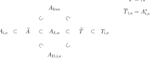
H1(Rn); cf. Proposition 3.7. For the relation between the operatorA_δ,α and the other operators studied in this section see Fig.1.

The following theorem contains a proof of self-adjointness of the operator