arXiv:1210.4709v2 [math.SP] 8 Nov 2012
SCHR ¨ODINGER OPERATORS WITH δ AND δ-POTENTIALS
SUPPORTED ON HYPERSURFACES
JUSSI BEHRNDT, MATTHIAS LANGER, AND VLADIMIR LOTOREICHIK
Abstract. Self-adjoint Schr¨odinger operators withδ and δ′-potentials
sup-ported on a smooth compact hypersurface are defined explicitly via boundary conditions. The spectral properties of these operators are investigated, regu-larity results on the functions in their domains are obtained, and analogues of the Birman–Schwinger principle and a variant of Krein’s formula are shown. Furthermore, Schatten–von Neumann type estimates for the differences of the powers of the resolvents of the Schr¨odinger operators withδandδ′-potentials,
and the Schr¨odinger operator without a singular interaction are proved. An immediate consequence of these estimates is the existence and completeness of the wave operators of the corresponding scattering systems, as well as the uni-tary equivalence of the absolutely continuous parts of the singularly perturbed and unperturbed Schr¨odinger operators. In the proofs of our main theorems we make use of abstract methods from extension theory of symmetric operators, some algebraic considerations and results on elliptic regularity.
1. Introduction
Schr¨odinger operators withδandδ′-potentials supported on hypersurfaces play an important role in mathematical physics and have attracted a lot of attention in the recent past; they are used for the description of quantum particles interacting with charged hypersurfaces. In this introduction we first define the differential operators which are studied in the present paper. Furthermore, we state and explain our main results on the spectral and scattering properties of these operators in an easily understandable but mathematically exact form in Theorems A–D below. Although the remaining part of the paper can be viewed as a proof of these theorems we mention that Sections3 and4 contain not only slightly generalized versions of Theorems A–D but also other results which are of independent interest.
In the following let Σ be a compact connectedC∞-hypersurface which separates the Euclidean spaceRn into a bounded domain Ωi and an unbounded domain Ωe with common boundary∂Ωe=∂Ωi= Σ. Denote byδΣtheδ-distribution supported on Σ and byδ′
Σ its normal derivative in the distributional sense with the normal pointing outwards of Ωi. The main objective of the present paper is to define and study the spectral properties of Schr¨odinger operators associated with the formal differential expressions
(1.1) Lδ,α:=−∆ +V −αδΣ,·δΣ and Lδ′,β :=−∆ +V −βδΣ′ ,·
δ′ Σ.
2010Mathematics Subject Classification. 35P05, 35P20, 47F05, 47L20, 81Q10, 81Q15.
Key words and phrases. Schr¨odinger operator, δ and δ′-potential, self-adjoint extension,
Schatten–von Neumann class, wave operators, absolutely continuous spectrum.
Here V ∈L∞(Rn) is assumed to be a real-valued potential andα, β: Σ →Rare real-valued measurable functions, often called strengths of interactions in math-ematical physics. In order to define the Schr¨odinger operators with δ and δ′ -interactions rigorously, it is necessary to specify suitable domains inL2(Rn) which take into account theδandδ′-interaction on the hypersurface Σ. In our approach this will be done explicitly via suitable interface conditions on Σ for a certain func-tion space in L2(Rn). One of the main advantages of our method compared with the usual approach via semi-bounded closed sesquilinear forms (see, e.g. [18,30]) is thatδ′-interactions can be treated without any additional difficulties.
Throughout the paper we write the functionsf ∈L2(Rn) in the formf =fi⊕fe with respect to the corresponding space decomposition L2(Ωi)⊕L2(Ωe). For the definition of Schr¨odinger operators withδorδ′-potentials we introduce the following subspaces
H∆3/2(Ωi) :=fi∈H3/2(Ωi) : ∆fi∈L2(Ωi) ,
H∆3/2(Ωe) :=fe∈H3/2(Ωe) : ∆fe∈L2(Ωe) ,
of the Sobolev spaces H3/2(Ωi) and H3/2(Ωe), respectively, and their orthogonal sum inL2(Rn):
H∆3/2(Rn\Σ) :=H∆3/2(Ωi)⊕H∆3/2(Ωe);
cf. [2, 59] and Sections 2.3 and 2.4 for more details. The trace of a function fi ∈ H∆3/2(Ωi) and the trace of the normal derivative ∂νifi (with the normal νi
pointing outwards) are denoted byfi|Σ and∂νifi|Σ, respectively. Similarly, for the
exterior domain andfe ∈H∆3/2(Ωe) we write fe|Σ and ∂νefe|Σ; here νe and νi are
pointing in opposite directions.
The main objects we study in this paper are the operators given in the following definition, which are associated with the formal differential expressions in (1.1).
Definition. Let α ∈ L∞(Σ) be a real-valued function on Σ. The Schr¨odinger
operator Aδ,αcorresponding to theδ-interaction with strengthαonΣis defined as
Aδ,αf :=−∆f+V f,
domAδ,α:= (
f ∈H∆3/2(Rn\Σ) : fi|Σ=fe|Σ αfi|Σ=∂νefe|Σ+∂νifi|Σ
) .
Let β be a real-valued function on Σ such that 1/β ∈ L∞(Σ). The Schr¨odinger
operatorAδ′,β corresponding to theδ′-interaction with strengthβ onΣis defined as Aδ′,βf :=−∆f+V f,
domAδ′,β:= (
f ∈H∆3/2(Rn\Σ) : ∂νefe|Σ=−∂νifi|Σ
β∂νefe|Σ=fe|Σ−fi|Σ
) .
The boundary conditions in the domains of Aδ,α and Aδ′,β fit with the formal differential expressions in (1.1). In order to see this forAδ,αwe introduce the closed symmetric form
aδ,α[f, g] = (∇f,∇g)L2(Rn;Cn)+ (V f, g)L2(Rn)−(αf|Σ, g|Σ)L2(Σ)
onH1(Rn). Further making use of the boundary conditionsfi|
yields
(Aδ,αf, g)L2(Rn)=aδ,α[f, g] =Lδ,αf, g
for all g ∈ H1(Rn). This also shows that Aδ,α coincides with the self-adjoint operator associated with the closed symmetric form aδ,α; cf. Proposition 3.7 for more details. The quadratic form method has been used in various papers for the definition of Schr¨odinger operators with δ-perturbations supported on curves and hypersurfaces. We refer the reader to [18] and the review paper [30] for more details and further references; we also mention [19,28,29,32,33,34,35,39,58] for studies of eigenvalues, [16, 31, 38, 70] for results on the absolutely continuous spectrum, and [6, 36, 37, 40, 41, 54, 60, 67] for related problems for Schr¨odinger operators with δ-perturbations. We point out that the quadratic form approach could not be adapted to the δ′-case so far; see the open problem posed in [30, 7.2] and our solution in Proposition 3.15. For completeness we also mention that the above definitions of the differential operatorsAδ,αandAδ′,β are compatible with the ones for one-dimensionalδandδ′-point interactions in [3,4].
In the next theorem, which is the first main result of this paper, we obtain some basic properties of the Schr¨odinger operatorsAδ,αandAδ′,β. Here also thefree or
unperturbed Schr¨odinger operator
Afreef =−∆f+V f, domAfree=H2(Rn),
is used. It is well known and easy to see thatAfreeis semi-bounded and self-adjoint in L2(Rn). Recall that the essential spectrum σess(A) of a self-adjoint operatorA consists of all spectral points that are not isolated eigenvalues of finite multiplicity. The statements in Theorem A below are contained in Theorems3.5,3.11,3.14and
3.16in Sections3.2–3.4.
Theorem A. The Schr¨odinger operators Aδ,αand Aδ′,β are self-adjoint operators
inL2(Rn), which are bounded from below, and their essential spectra satisfy σess(Aδ,α) =σess(Aδ′,β) =σess(Afree).
If V ≡ 0, then σess(Aδ,α) = σess(Aδ′,β) = [0,∞) and the negative spectra of the
self-adjoint operators Aδ,α and Aδ′,β consist of finitely many negative eigenvalues
with finite multiplicities.
It is not surprising that additional smoothness assumptions on the functionsα andβin the boundary condition yield more regularity for the functions in domAδ,α and domAδ′,β. The H2-case is of particular importance; see also [17] where the Laplacian on a strip was considered. The next theorem follows from Theorems3.6
and 3.12. The Sobolev space of order one of L∞-functions on Σ is denoted by W1,∞(Σ).
Theorem B. If α∈W1,∞(Σ), thendomAδ,α is contained in H2(Ωi)⊕H2(Ωe).
If 1/β∈W1,∞(Σ), thendomAδ
′,β is contained inH2(Ωi)⊕H2(Ωe).
The fact that the essential spectra of the operators Aδ,α, Aδ′,β and Afree in Theorem A coincide, follows from the observation that the resolvent differences of these operators are compact. Roughly speaking this is a consequence of the compactness of the hypersurface Σ and Sobolev embedding theorems. However, as can be expected from the classical results in [12] (see also [10,13,14,23,49,52,53,
in turn imply existence and completeness of the wave operators of the scattering pairs {Aδ,α, Afree} and {Aδ′,β, Afree}; see, e.g. [56, 65, 72] for more details and consequences.
Recall that a compact operator T is said to belong to the weak Schatten–von Neumann ideal Sp,∞ if the sequence of singular values sk, i.e. the sequence of eigenvalues of the non-negative operator (T∗T)1/2, satisfiessk=O(k−1/p),k→ ∞. Note thatSp,∞⊂Sp′for allp′> p, whereSp′ is the usual Schatten–von Neumann ideal; cf. Section2.1.
Theorem C. For the self-adjoint Schr¨odinger operatorsAδ,α andAδ′,β in L2(Rn)
the following statements hold.
(i) For allλ∈ρ(Aδ,α)∩ρ(Afree)we have
(Aδ,α−λ)−1−(Afree−λ)−1∈Sn−1
3 ,∞
and, in particular, the wave operators for the pair {Aδ,α, Afree} exist and are complete whenn= 2 orn= 3.
(ii) For allλ∈ρ(Aδ′,β)∩ρ(Afree)we have
(Aδ′,β−λ)−1−(Afree−λ)−1∈Sn−1 2 ,∞,
and, in particular, the wave operators for the pair {Aδ′,β, Afree} exist and
are complete whenn= 2.
The scattering theory for operators withδ-potentials in the two-dimensional case is partially developed in [36]. In higher dimensions it is necessary to extend the estimates to higher powers of resolvents as we do in the next main theorem un-der an additional local regularity assumption on the potential V. In particular, for sufficiently smooth V this implies the existence and completeness of the wave operators for the scattering pairs {Aδ,α, Afree} and {Aδ′,β, Afree} in any space di-mension. Fork ∈N0 the subspace of L∞(Rn) which consists of all functions that admit partial derivatives in an open neighbourhood of the hypersurface Σ up to orderkin L∞(Rn) is denoted byWk,∞
Σ (Rn).
Theorem D. Let the self-adjoint Schr¨odinger operatorsAδ,αandAδ′,β be as above,
and assume that V ∈ WΣ2m−2,∞(Rn) for some m ∈N. Then the following state-ments hold.
(i) For alll= 1,2, . . . , mandλ∈ρ(Aδ,α)∩ρ(Afree)we have
(Aδ,α−λ)−l−(Afree−λ)−l∈Sn−1 2l+1,∞,
and, in particular, the wave operators for the pair {Aδ,α, Afree} exist and are complete when2m−2> n−4.
(ii) For alll= 1,2, . . . , mandλ∈ρ(Aδ′,β)∩ρ(Afree)we have (Aδ′,β−λ)−l−(Afree−λ)−l∈Sn−1
2l ,∞,
and, in particular, the wave operators for the pair {Aδ′,β, Afree} exist and
are complete when2m−2> n−3.
The paper is organized as follows. Section 2 contains preliminary material on Schatten–von Neumann classes, general extension theory of symmetric operators and function spaces. In particular, we prove some useful abstract lemmas on re-solvent power differences in Section 2.1. Furthermore, in Section 2.2 we collect basic facts about quasi boundary triples — a convenient abstract tool from [8,9] to study self-adjoint extensions of symmetric partial differential operators — and recall a variant of Krein’s formula suitable for our purposes. Section 3 is devoted to the rigorous mathematical definition and the investigation of the spectral prop-erties of the operatorsAδ,αandAδ′,β. In Sections3.2and3.3we provide proofs of self-adjointness and sufficient conditions forH2-regularity of the operator domains, cf. Theorems A and B, and we discuss variants of the Birman–Schwinger principle for the description of eigenvalues of the self-adjoint operatorsAδ,α and Aδ′,β. All these results are obtained by means of suitable quasi boundary triples constructed in these sections. Section3.2is accompanied by a comparison with the sesquilinear form approach to Schr¨odinger operators withδ-potentials on hypersurfaces. In Sec-tion3.4 we obtain basic spectral properties of the self-adjoint operators Aδ,α and Aδ′,β such as lower semi-boundedness and finiteness of negative spectra if V ≡0. Section4contains our main results on Schatten–von Neumann estimates from The-orems C and D for resolvent power differences of operatorsAδ,α,Aδ′,βandAfree. As a direct consequence of these estimates we establish the existence and completeness of wave operators for certain scattering pairs arising in quantum mechanics.
We emphasize again that the results in the body of the paper are sometimes stronger than in the introduction. Several theorems of their own independent in-terest are formulated only in the main part. We also mention that many of the results in the paper extend to more general second order differential operators with sufficiently smooth coefficients and also remain to be true under weaker assump-tions on the smoothness of the hypersurface Σ; in this context we refer the reader to the recent papers [1, 7, 43, 44, 45, 46, 63] on elliptic operators in non-smooth domains.
2. Preliminaries
This section contains some preliminary material that will be used in the main part of the paper. In Section2.1we first recall some basic properties of Schatten– von Neumann ideals and we prove an abstract lemma with sufficient conditions for resolvent power differences to belong to some Schatten–von Neumann class. The concept of quasi boundary triples and their Weyl functions from general extension theory of symmetric operators is briefly reviewed in Section2.2. Sections2.3and2.4
contain mainly definitions and notations for the function spaces used in the paper.
2.1. SpandSp,∞-classes. LetHandGbe separable Hilbert spaces. The space of bounded everywhere defined linear operators fromHintoGis denoted byB(H,G), and we set B(H) := B(H,H). The ideal of compact operators mapping from H
The Schatten–von Neumann class of operator idealsSpand the weak Schatten–von Neumann class of operator idealsSp,∞are defined as
Sp:=
T∈S∞: ∞ X
k=1
sk(T)p<∞
,
Sp,∞:=nT ∈S∞:sk(T) =O(k−1/p), k→ ∞o,
p >0;
they play an important role later on. We refer the reader to [47, III.§7 and III.§14], [69, Chapter 2] and to [15, Chapter 11] for a detailed study of the classesSp and Sp,∞. If a compact operatorT ∈S∞(H,G) belongs to Sp or Sp,∞, then we also write T ∈ Sp(H,G) orT ∈ Sp,∞(H,G), respectively, if the spaces H and G are important in the context. Moreover, we set
Sp·Sq :=T1T2:T1∈Sp, T2∈Sq ,
Sp,∞·Sq,∞:=T1T2:T1∈Sp,∞, T2∈Sq,∞ .
The proof of the next statement can be found in [15,47] and, e.g. [11, Lemma 2.3].
Lemma 2.1. Let p, q, r, s, t >0. Then the following statements are true:
(i) Sp·Sq =Sr andSp,∞·Sq,∞=Sr,∞ whenp−1+q−1=r−1, or,
equiva-lently
S1
s ·S1t =Ss+1t and Ss1,∞·S1t,∞=Ss1+t,∞;
(ii) If T ∈Sp, thenT∗∈Sp; if T ∈Sp,∞, thenT∗∈Sp,∞; (iii) Sp⊂Sp,∞ andSp′,∞⊂Sp for allp′< p.
LetH andK be linear operators in a separable Hilbert spaceHand assume that ρ(H)∩ρ(K)6=∅. In order to investigate properties of the difference of the mth powers of the resolvents,
(H−λ)−m−(K−λ)−m, λ∈ρ(H)∩ρ(K), m∈N,
recall that, for two elementsaandbof some non-commutative algebra, the following formula holds:
(2.1) am−bm=
m−1X
k=0
am−k−1 a−bbk.
Substituting aandbby the resolvents ofH andK, respectively, and setting (2.2) Tm,k(λ) := (H−λ)−(m−k−1)(H−λ)−1−(K−λ)−1(K−λ)−k forλ∈ρ(H)∩ρ(K),m∈Nandk= 0,1, . . . , m−1, we conclude from (2.1) that
(2.3) (H−λ)−m−(K−λ)−m= m−1X
k=0
Tm,k(λ)
Lemma 2.2. Let H andK be linear operators inH such thatρ(H)∩ρ(K)6=∅. Moreover, let p >0,m∈Nand Tm,k be as in (2.2), and assume that Tm,k(λ0)∈
Sp,∞(H) for someλ0∈ρ(H)∩ρ(K)and all k= 0,1, . . . , m−1. Then
(H−λ)−m−(K−λ)−m∈Sp,∞(H)
for allλ∈ρ(H)∩ρ(K).
Proof. Forλ∈ρ(H)∩ρ(K) define
(2.4) Eλ:=I+ (λ−λ0)(H−λ)−1 and Fλ:=I+ (λ−λ0)(K−λ)−1. The resolvent identity implies that
(2.5) Eλ(H−λ0)−1= (H−λ0)−1+ (λ−λ0)(H−λ)−1(H−λ0)−1= (H−λ)−1 and, similarly,
(2.6) (K−λ0)−1Fλ= (K−λ)−1. By induction we obtain
(2.7) Eλl(H−λ0)−l= (H−λ)−l and (K−λ0)−lFλl = (K−λ)−l
for alll∈N. SetD1(λ) := (H−λ)−1−(K−λ)−1,λ∈ρ(H)∩ρ(K). Then (2.5), (2.6) and (2.4) imply that
EλD1(λ0)Fλ =Eλ(H−λ0)−1Fλ−Eλ(K−λ0)−1Fλ = (H−λ)−1Fλ−Eλ(K−λ)−1
= (H−λ)−1+ (λ−λ0)(H−λ)−1(K−λ)−1
−(K−λ)−1−(λ−λ0)(H−λ)−1(K−λ)−1 =D1(λ).
(2.8)
Fork= 0,1. . . , m−1 and allλ∈ρ(H)∩ρ(K) we obtain from (2.7), (2.8) and the facts thatEλ commutes with (H−λ0)−1 andFλ commutes with (K−λ0)−1 the following relation
Tm,k(λ) = (H−λ)−(m−k−1)D1(λ)(K−λ)−k = (H−λ)−(m−k−1)EλD1(λ0)Fλ(K−λ)−k
=Eλm−k−1(H−λ0)−(m−k−1)EλD1(λ0)Fλ(K−λ0)−kFk λ
=Eλm−k(H−λ0)−(m−k−1)D1(λ0)(K−λ0)−kFλk+1 =Eλm−kTm,k(λ0)Fλk+1.
By assumption,Tm,k(λ0)∈Sp,∞, and hence we conclude thatTm,k(λ)∈Sp,∞for k= 0,1, . . . , m−1 andλ∈ρ(H)∩ρ(K). This together with (2.3) implies that
(H−λ)−m−(K−λ)−m= m−1X
k=0
Tm,k(λ)∈Sp,∞(H)
for allλ∈ρ(H)∩ρ(K).
Lemma 2.3. Let H andK be linear operators in H, let Kbe an auxiliary Hilbert space and assume that, for some λ0 ∈ ρ(H)∩ρ(K), there exist operators B ∈ B(K,H)andC∈ B(H,K) such that
(2.9) (H−λ0)−1−(K−λ0)−1=BC.
Leta >0andb1, b2≥0be such thata≤b1+b2 and setb:=b1+b2−a. Moreover, letr∈Nand assume that
(2.10)
(K−λ0)−kB∈S 1
ak+b1,∞,
C(K−λ0)−k∈S 1
ak+b2,∞,
k= 0,1, . . . , r−1.
Then
(2.11) (H−λ)−l−(K−λ)−l∈S
1
al+b,∞ for allλ∈ρ(H)∩ρ(K)and all l= 1,2, . . . , r.
Proof. We prove the statement by induction with respect tol. Using the factoriza-tion in (2.9), the assumptions in (2.10) withk= 0 and Lemma2.1(i) we obtain
(H−λ0)−1−(K−λ0)−1=BC∈S1
b1,∞·S 1
b2,∞=S 1
b1 +b2,∞=S 1
a+b,∞.
Now Lemma2.2 withm= 1 implies that
(H−λ)−1−(K−λ)−1∈S
1
a+b,∞
for allλ∈ρ(H)∩ρ(K), i.e. (2.11) is true forl= 1.
For the induction step fixm∈N, 2≤m≤rand assume that (2.11) is satisfied for alll= 1,2, . . . , m−1. Fork= 0,1, . . . , m−1 letTm,kbe as in (2.2), define
Dj(λ0) := (H−λ0)−j−(K−λ0)−j, j ∈N0, and write
(2.12)
Tm,k(λ0) = (H−λ0)−(m−k−1)BC(K−λ0)−k =Dm−k−1(λ0)BC(K−λ0)−k
+ (K−λ0)−(m−k−1)BC(K−λ0)−k. Note thatD0(λ0) = 0. By assumption (2.10) we have
B∈S1
b1,∞, C(K−λ0)
−k ∈ S 1
ak+b2,∞,
(K−λ0)−(m−k−1)B∈S 1
a(m−k−1)+b1,∞,
fork= 0,1, . . . , m−1. By the induction assumption we also have Dm−k−1(λ0)∈S 1
a(m−k−1)+b,∞
fork= 0,1, . . . , m−1, and and hence we obtain with Lemma2.1(i) that the first summand in (2.12) is in
S 1
a(m−k−1)+b,∞·Sb11,∞·Sak+1b2,∞=Sam1+2b,∞⊂Sam1+b,∞,
where we used thatb≥0. The second summand in (2.12) is in S 1
a(m−k−1)+b1,∞·S 1
ak+b2,∞=S 1
am+b,∞.
HenceTm,k(λ0)∈S 1
am+b,∞for allk= 0,1, . . . , m−1. Now Lemma2.2implies the
2.2. Quasi boundary triples and their Weyl functions. The concept of quasi boundary triples and Weyl functions is a generalization of the notion of (ordinary) boundary triples and Weyl functions from [20, 26, 48, 57], which is a very con-venient tool in extension theory of symmetric operators. Quasi boundary triples are particularly useful when dealing with elliptic boundary value problems from an operator and extension theoretic point of view. In this subsection we provide some general facts on quasi boundary triples which can be found in [8] and [9].
Throughout this subsection let (H,(·,·)H) be a Hilbert space and let A be a densely defined closed symmetric operator inH.
Definition 2.4. A triple {G,Γ0,Γ1} is called a quasi boundary triple for A∗ if (G,(·,·)G) is a Hilbert space and for some linear operatorT ⊂A∗ withT =A∗the following holds:
(i) Γ0,Γ1: domT → G are linear mappings and ran Γ0
Γ1
is dense inG × G;
(ii) A0:=T ↾ker Γ0 is a self-adjoint operator inH; (iii) for all f, g∈domT theabstract Green’s identityholds: (2.13) (T f, g)H−(f, T g)H= (Γ1f,Γ0g)G−(Γ0f,Γ1g)G.
The following simple example illustrates the notion of quasi boundary triples for the Laplacian on a smooth bounded domain, see [8, 9], Section 3.1 and Proposi-tion3.1.
Example. Let Ω be a bounded domain with smooth boundary, A = −∆ with domA =H2
0(Ω), T = −∆ with domT =H2(Ω), let G =L2(∂Ω) and define the boundary mappings as
Γ0f =∂νf|∂Ω, Γ1f =f|∂Ω, f ∈domT;
where∂ν stands for the normal derivative with normal vector pointing outwards. It can be shown that the closure ofT coincides with the adjoint operatorA∗ =−∆, domA∗ = {f ∈ L2(Ω) : ∆f ∈ L2(Ω)}, and that the properties of (i)-(iii) in Definition 2.4hold. Hence{L2(∂Ω),Γ0,Γ1}is a quasi boundary triple for A∗.
We remark that a quasi boundary triple for the adjointA∗ of a densely defined closed symmetric operator exists if and only if the deficiency indices n±(A) = dim ker(A∗∓i) ofAcoincide. Moreover, if{G,Γ0,Γ1}is a quasi boundary triple for A∗, thenAcoincides withT ↾(ker Γ0∩ker Γ1) and the operatorA1:=T ↾ker Γ1is symmetric inH. We also mention that a quasi-boundary triple with the additional property ran Γ0=Gis a generalized boundary triple in the sense of [25,27]. In the special case that the deficiency indicesn±(A) ofAare finite (and coincide) a quasi boundary triple is automatically an ordinary boundary triple.
The following proposition contains a sufficient condition for a triple{G,Γ0,Γ1}
to be a quasi boundary triple, cf. [8, Theorem 2.3] and [9, Theorem 2.3]. The result will be applied in Sections3.2 and3.3.
Proposition 2.5. Let HandG be Hilbert spaces and letT be a linear operator in
H. Assume that Γ0,Γ1: domT → G are linear mappings such that the following conditions are satisfied:
(a) The range of Γ0
Γ1
(b) The identity (2.13)holds for allf, g∈domT.
(c) T ↾ker Γ0 is an extension of a self-adjoint operator A0.
Then A:=T ↾ker Γ0∩ker Γ1 is a densely defined closed symmetric operator inH, and{G,Γ0,Γ1}is a quasi boundary triple for A∗ with A0=T ↾ker Γ0.
Next we recall the definition of theγ-field and the Weyl function associated with a quasi boundary triple{G,Γ0,Γ1}forA∗. Note first that the decomposition
domT = domA0+ ker(T˙ −λ) = ker Γ0+ ker(T˙ −λ)
holds for allλ∈ρ(A0). Hence Γ0 ↾ker(T−λ) is invertible for allλ∈ρ(A0) and maps ker(T−λ) bijectively onto ran Γ0.
Definition 2.6. Let{G,Γ0,Γ1} be a quasi boundary triple forT =A∗ andA0= T ↾ker Γ0. Then the (operator-valued) functionsγandM defined by
γ(λ) := Γ0↾ker(T−λ)−1 and M(λ) := Γ1γ(λ), λ∈ρ(A0),
are called theγ-field and theWeyl function corresponding to the quasi boundary triple{G,Γ0,Γ1}.
The values of the Weyl function corresponding to the quasi boundary triple
{L2(∂Ω),Γ0,Γ1} in the example below Definition 2.4 are Neumann-to-Dirichlet maps; cf. [8,9], Section3.1and Proposition3.1.
The definitions of γ and M coincide with the definitions of the γ-field and the Weyl function in the case that{G,Γ0,Γ1} is an ordinary boundary triple, cf. [26]. Note that, for eachλ∈ρ(A0), the operatorγ(λ) maps ran Γ0intoHandM(λ) maps ran Γ0into ran Γ1. Furthermore, as an immediate consequence of the definition of M(λ) we obtain
M(λ)Γ0fλ= Γ1fλ, fλ∈ker(T −λ), λ∈ρ(A0).
In the next proposition we collect some properties of the γ-field and the Weyl function; all statements are proved in [8].
Proposition 2.7. Let {G,Γ0,Γ1} be a quasi boundary triple for T = A∗ with A0 = T ↾ ker Γ0, γ-field γ and Weyl function M. Then, for λ ∈ ρ(A0), the following assertions hold.
(i) γ(λ)is a densely defined bounded operator fromG intoHwith domγ(λ) = ran Γ0.
(ii) The adjoint of γ(λ)satisfies
γ(λ)∗= Γ1(A0−λ)−1∈ B(H,G).
(iii) The values of the Weyl function M are densely defined (in general un-bounded) operators inG with domM(λ) = ran Γ0 andranM(λ)⊂ran Γ1. Furthermore,M(λ)⊂M(λ)∗ holds.
(iv) If ran Γ0=G, then M(λ)∈ B(G).
(v) If A1 =T ↾ ker Γ1 is a self-adjoint operator in Hand λ∈ρ(A0)∩ρ(A1), thenM(λ)is a bijective mapping fromran Γ0 ontoran Γ1.
ofT ⊂A∗. The extensionsAΘ are defined with the help of an abstract boundary condition by
(2.14) AΘ:=T ↾ker Γ1−ΘΓ0=T↾ker Θ−1Γ1−Γ0,
where Θ is a linear operator inGor a linear relation inG, i.e. a subspace ofG × G, cf. [8]. The sums and products are understood in the sense of linear relations if Θ or Θ−1 is not a (single-valued) operator. However, for our purposes the case that Θ−1is a bounded linear operator onG is of particular interest and linear relations will not be used in the following. The next statement contains a variant of Krein’s formula in this case; see [8, Theorem 2.8 and Theorem 4.8], [9, Theorem 3.7 and Corollary 3.9] and [11, Theorem 3.13].
Theorem 2.8. Let{G,Γ0,Γ1}be a quasi boundary triple forT =A∗ withA0=T ↾ ker Γ0,γ-field γ and Weyl function M. Furthermore, let B =B∗ = Θ−1 ∈ B(G)
and let
(2.15) AΘ=T ↾ker BΓ1−Γ0
be the corresponding extension as in (2.14). Then, for λ ∈ ρ(A0), the following assertions hold.
(i) λ∈σp(AΘ) if and only if ker(I−BM(λ))6={0}. Moreover, in this case, the multiplicity of the eigenvalueλof AΘ is equal to dim ker(I−BM(λ)).
(ii) For allg∈ran(AΘ−λ)andλ /∈σp(AΘ) we have
(AΘ−λ)−1g−(A0−λ)−1g=γ(λ) I−BM(λ)−1Bγ(λ)∗g.
If, in addition, ran Γ0 =G and M(λ0) ∈ S∞(G) for some λ0 ∈ C\R, then the operator AΘ in (2.15)is self-adjoint in H, Krein’s formula
(2.16) (AΘ−λ)−1−(A0−λ)−1=γ(λ) I−BM(λ)−1Bγ(λ)∗
holds for allλ∈ρ(AΘ)∩ρ(A0), and(I−BM(λ))−1∈ B(G).
2.3. Sobolev spaces, traces and Green’s identities. Throughout this paper Sobolev spaces and certain interpolation spaces play an important role. In this subsection we provide some necessary definitions and basic properties. The reader is referred, e.g. to the monographs [2, 51,59,62] for more details.
Let Ω⊂Rnbe an arbitrary bounded or unbounded domain with a compactC∞ -boundary∂Ω). ByHs(Ω) and Hs(∂Ω),s∈R, we denote the standard (L2-based) Sobolev spaces of ordersof functions in Ω and∂Ω, respectively. The inner product and norm onHsare denoted by (·,·)sandk · ks, fors= 0 we simply write (·,·) and
k · k, respectively. In order to avoid possible confusion, sometimes also the space is used as an index, e.g. (·,·)L2(Ω) and (·,·)L2(∂Ω). The Sobolev spaces of order
k ∈ N0 of L∞-functions on Ω and ∂Ω are denoted by Wk,∞(Ω) and Wk,∞(∂Ω), respectively. The following well-known implications will be used later:
(2.17) f ∈H
k(Ω), g∈Wk,∞(Ω) =⇒ f g∈Hk(Ω), k∈N0; h∈H1(∂Ω), k∈W1,∞(∂Ω) =⇒ hk∈H1(∂Ω).
For a function f on Ω we denote by f|∂Ω and ∂νf|∂Ω the trace and the trace of the normal derivative (with normal vector pointing outwards), respectively. For s >3/2 the trace mapping
is the continuous extension of the trace mapping defined on C∞-functions. Recall that fors >3/2 the mapping (2.18) is surjective onto Hs−1/2(∂Ω)×Hs−3/2(∂Ω).
Besides the Sobolev spacesHs(Ω) the spaces H∆s(Ω) :=
f ∈Hs(Ω) : ∆f ∈L2(Ω) , s≥0,
equipped with the inner product (·,·)s+ (∆·,∆·) and corresponding norm will be useful. Observe that fors≥2 the spacesHs
∆(Ω) andHs(Ω) coincide. We also note thatHs
∆(Ω),s∈(0,2), can be viewed as an interpolation space betweenH2(Ω) and H0
∆(Ω), where the latter space coincides with the maximal domain of the Laplacian inL2(Ω). By [59] the trace mapping can be extended to a continuous mapping (2.19) H∆s(Ω)∋f 7→
f|∂Ω, ∂νf|∂Ω ∈Hs−1/2(∂Ω)×Hs−3/2(∂Ω) for alls∈[0,2), where each of the mappings
H∆s(Ω)∋f 7→f|∂Ω∈Hs−1/2(∂Ω), H∆s(Ω)∋f 7→∂νf|∂Ω∈Hs−3/2(∂Ω)
is surjective fors∈[0,2). We also recall that the first and second Green’s identities hold for allf, g∈H∆3/2(Ω) andh∈H1(Ω):
(2.20) −∆f, hL2(Ω)= ∇f,∇h
L2(Ω;Cn)− ∂νf|∂Ω, h|∂Ω
L2(∂Ω)
and
−∆f, gL2(Ω)− f,−∆g
L2(Ω)
= f|∂Ω, ∂νg|∂ΩL2(∂Ω)− ∂νf|∂Ω, g|∂Ω
L2(∂Ω),
(2.21)
cf. [42,59] and, e.g. [11, Theorem 4.2].
2.4. Some local Sobolev spaces. Let Σ be a compact connectedC∞-hypersurface which separates the Euclidean spaceRn into a bounded (interior) domain Ωi and an unbounded (exterior) domain Ωe. In particular, Σ =∂Ωi =∂Ωe. For s≥0 we use the short notation
(2.22) Hs(Rn\Σ) :=Hs(Ωi)⊕Hs(Ωe) and H∆s(Rn\Σ) :=H∆s(Ωi)⊕H∆s(Ωe). We denote by Hs
Σ(Ωi) with s ≥ 0 the subspace of L2(Ωi) which consists of functions that belong toHs in a neighbourhood of Σ =∂Ωi, i.e.
HΣs(Ωi) :=
f ∈L2(Ωi) :∃domain Ω′ ⊂Ωi such that
∂Ω′⊃Σ andf ↾Ω′∈Hs(Ω′) . The space Hs
Σ(Ωe) is defined in the same way with Ωi replaced by Ωe. The local Sobolev spacesHs
Σ(Rn) andHΣs(Rn\Σ) in the next definition consist ofL2-functions which areHs in a neighbourhood of Σ or in both one-sided neighbourhoods of Σ, respectively.
Definition 2.9. Let Σ, Ωi, Ωe, and the spaces Hs
Σ(Ωi) and HΣs(Ωe), s≥0, be as above. Then we define
HΣs(Rn) :=
f ∈L2(Rn) :∃ domain Ω′⊂Rn such that
It follows from the above definition that Hs
Σ(Rn) ( HΣs(Rn\Σ) holds for all s >0.
For k∈ N0 we denote by WΣk,∞(Ωi) the subspace ofL∞(Ωi) which consists of functions that belong toWk,∞ in a neighbourhood of Σ =∂Ωi, i.e.
WΣk,∞(Ωi) :=
f ∈L∞(Ωi) :∃domain Ω′ ⊂Ωi such that
∂Ω′⊃Σ andf ↾Ω′∈Wk,∞(Ω′) . The spaceWΣk,∞(Ωe) is defined in the same way with Ωi replaced by Ωe. In analogy to Definition2.9we introduce the local Sobolev spacesWΣk,∞(Rn) andWk,∞
Σ (Rn\Σ) ofL∞-functions which belong toWk,∞in a neighbourhood or both one-sided neigh-bourhoods of Σ, respectively.
Definition 2.10. Let Σ, Ωi, Ωe, and the spacesWΣk,∞(Ωi) andWΣk,∞(Ωe),k∈N0, be as above. Then we define
WΣk,∞(Rn) :=f ∈L∞(Rn) :∃domain Ω′⊂Rn such that
Ω′⊃Σ andf ↾Ω′∈Wk,∞(Ω′) , WΣk,∞(Rn\Σ) :=WΣk,∞(Ωi)×WΣk,∞(Ωe).
Finally, we recall a well-known result about theSp,∞ property of bounded op-erators mapping into the Sobolev spaceHq2(Σ), whereq2>0 and Σ =∂Ωi =∂Ωe
is the (n−1)-dimensional compact connectedC∞-hypersurface from above, cf. [50] and [11, Lemma 4.6].
Lemma 2.11. Let K be a Hilbert space, B∈ B(K, L2(Σ)) and letq2> q1 ≥0. If ranB⊂Hq2(Σ), thenB belongs to the class S n
−1
q2−q1,∞(K, H
q1(Σ)).
3. Self-adjoint Schr¨odinger operators with interactions on hypersurfaces
In this section we define the Schr¨odinger operators withδandδ′-interactions on hypersurfaces with the help of quasi boundary triple techniques. These definitions coincide with the ones in the introduction and are compatible with those for one-dimensional δ-point interactions from [3,4] and the definition ofδ-interactions on manifolds via quadratic forms; see, e.g. [18,35,39,41,58]. We also determine the semi-bounded closed quadratic form which corresponds to the Schr¨odinger operator with aδ′-interaction on a hypersurface, which answers a question from [30] posed by P. Exner. As a byproduct of the quasi boundary triple approach we obtain variants of Krein’s formula and the Birman–Schwinger principle. This section contains the complete proofs of Theorem A and Theorem B from the introduction.
3.1. Notations and preliminary facts. Let Σ be a compact connected C∞ -hypersurface which separates the Euclidean space Rn, n ≥ 2, into a bounded (interior) domain Ωi and an unbounded (exterior) domain Ωe with the common boundary∂Ωi=∂Ωe= Σ. Let
(3.1) L=−∆ +V,
where V is a real-valued potential from L∞(Rn). The restrictions of L to the interior and exterior domains will be denoted, respectively, by
For a functionf ∈L2(Rn) we writef =fi⊕fe, wherefi=f ↾Ωi andfe=f ↾Ωe. Let us denote by (·,·), (·,·)i, (·,·)e and (·,·)Σ the inner products in the Hilbert spacesL2(Rn),L2(Ωi),L2(Ωe) and L2(Σ), respectively. When it is clear from the context, we denote the inner products in the Hilbert spacesL2(Rn;Cn),L2(Ωi;Cn), andL2(Ωe;Cn) of vector-valued functions also by (·,·), (·,·)iand (·,·)e, respectively. The minimal operators associated with the differential expressionsLiandLeare defined by
Aifi=Lifi, domAi=H02(Ωi), Aefe=Lefe, domAe=H02(Ωe).
The operatorsAi andAeare densely defined closed symmetric operators with infi-nite deficiency indices inL2(Ωi) andL2(Ωe), respectively. Hence their direct sum (3.2) Ai,e=Ai⊕Ae, domAi,e=H02(Ωi)⊕H02(Ωe),
is a densely defined closed symmetric operator with infinite deficiency indices in the spaceL2(Rn) =L2(Ωi)⊕L2(Ωe). Furthermore, we introduce the operators
Tifi=Lifi, domTi =H∆3/2(Ωi), Tefe=Lefe, domTe =H∆3/2(Ωe), and their direct sum
Ti,e=Ti⊕Te, domTi,e=H∆3/2(Rn\Σ), where the notation in (2.22) is used. It can be shown that A∗
i = Ti, A∗e = Te, and hence A∗i,e = Ti,e. Next we define the usual self-adjoint Dirichlet and Neu-mann realizations of the differential expressions Li and Le in L2(Ωi) and L2(Ωe), respectively:
AD,ifi=Lifi, domAD,i =fi∈H2(Ωi) :fi|Σ= 0 , AD,efe=Lefe, domAD,e =fe∈H2(Ωe) :fe|Σ= 0 ,
AN,ifi=Lifi, domAN,i =fi∈H2(Ωi) :∂νifi|Σ= 0 ,
AN,efe=Lefe, domAN,e =fe∈H2(Ωe) :∂νefe|Σ= 0 ,
and their direct sums
(3.3) AD,i,e =AD,i⊕AD,e,
domAD,i,e =f ∈H2(Rn\Σ) :fi|Σ=fe|Σ= 0 , and
(3.4) AN,i,e=AN,i⊕AN,e,
domAN,i,e=f ∈H2(Rn\Σ) :∂νifi|Σ=∂νefe|Σ= 0 ,
which are self-adjoint operators inL2(Rn). Finally, we denote the usual self-adjoint (free) realization ofL inL2(Rn) by
(3.5) Afreef =Lf, domAfree=H2(Rn).
In the next proposition we define quasi boundary triples for A∗
Proposition 3.1. LetAi,Ae,Ti,Te,AD,i,AD,e,AN,i andAN,e be as above. Then the following statements hold for j= iandj= e.
(i) The tripleΠj ={L2(Σ),Γ0,j,Γ1,j}, where
Γ0,jfj =∂νjfj|Σ, Γ1,jfj =fj|Σ, fj∈domTj=H
3/2 ∆ (Ωj),
is a quasi boundary triple for A∗
j. The restrictions of Tj to the kernels of
the boundary mappings are the Neumann and Dirichlet operators:
Tj↾ker Γ0,j=AN,j, Tj↾ker Γ1,j=AD,j;
the ranges of the boundary mappings are
ran Γ0,j=L2(Σ) and ran Γ1,j=H1(Σ). (ii) For λ∈ρ(AN,j)and ϕ∈L2(Σ) the boundary value problem
(Lj−λ)fj = 0, ∂νjfj|Σ=ϕ,
(3.6)
has the unique solutionγj(λ)ϕ∈H∆3/2(Ωj), where γj is theγ-field associ-ated withΠj. Moreover,γj(λ)is bounded fromL2(Σ) intoL2(Ωj). (iii) For λ∈ρ(AN,j)the Weyl functionMj associated with Πj is given by
Mj(λ)ϕ=fj|Σ, ϕ∈L2(Σ),
where fj = γj(λ)ϕ is the solution of (3.6). The operators Mj(λ) are bounded from L2(Σ) to H1(Σ) and compact in L2(Σ). If, in addition, λ∈ρ(AD,j), thenMj(λ)is a bijective map from L2(Σ)onto H1(Σ). The operatorsMi(λ) andMe(λ) in Proposition3.1(iii) are the Neumann-to-Dirichlet maps associated with the differential expressionsLi−λandLe−λ, respectively.
3.2. Schr¨odinger operators with δ-interactions on hypersurfaces: self-adjointness, Krein’s formula andH2-regularity. In this section we make use of quasi boundary triples to define and study the Schr¨odinger operatorAδ,α asso-ciated with the formal differential expressionLδ,α=−∆ +V−αhδΣ,· iδΣin (1.1). It is convenient to use the symmetric extension
(3.7) Ae:=Afree∩AD,i,e=L↾f ∈H2(Rn) :fi|Σ=fe|Σ= 0
of the orthogonal sum Ai,e in (3.2) as the underlying symmetric operator for the quasi boundary triple. Furthermore,
(3.8) Te:=Ti,e↾fi⊕fe∈H∆3/2(Rn\Σ) :fi|Σ=fe|Σ .
acts as the operator on whose domain boundary mappings are defined in the next proposition. The method of intermediate extensions is inspired by the general considerations for ordinary boundary triples in [24, Section 4]. We remark that the quasi boundary triple and Weyl function below appear also implicitly in [5] and [66, Section 4] in a different context.
Proposition 3.2. Let the operators Ae, Te,AD,i,e, AN,i,e andAfree be as in (3.7),
(i) The tripleΠ =e {L2(Σ),eΓ0,Γ1e }, where e
Γ0f =∂νefe|Σ+∂νifi|Σ, Γ1fe =f|Σ, f =fi⊕fe∈domT ,e
is a quasi boundary triple for Ae∗. The restrictions of Te to the kernels of
the boundary mappings are
e
T ↾kerΓ0e =Afree and Te↾kereΓ1=AD,i,e,
and the ranges of the boundary mappings are
(3.9) raneΓ0=L2(Σ) and raneΓ1=H1(Σ). (ii) For λ∈ρ(Afree)and ϕ∈L2(Σ) the transmission problem (3.10) (L −λ)f = 0, fe|Σ=fi|Σ, ∂νefe|Σ+∂νifi|Σ=ϕ,
has the unique solution eγ(λ)ϕ∈H∆3/2(Rn\Σ), where eγ is the γ-field asso-ciated with Πe. Moreover, eγ(λ)is bounded fromL2(Σ) toL2(Rn).
(iii) Forλ∈ρ(Afree)the valuesMf(λ)of the Weyl function associated withΠe are bounded operators from L2(Σ) to H1(Σ) and compact operators in L2(Σ).
If, in addition, λ ∈ ρ(AD,i,e), then Mf(λ) is a bijective map from L2(Σ)
ontoH1(Σ). Moreover, the identity
(3.11) Mf(λ) = Mi(λ)−1+Me(λ)−1−1
holds for allλ∈ρ(Afree)∩ρ(AD,i,e)∩ρ(AN,i,e).
Proof. (i) First note that the boundary mappingsΓ0,e eΓ1are well defined because of the properties of the trace mappings (2.19). We show that the tripleΠ satisfies thee conditions (a), (b) and (c) in Proposition2.5. For condition (a), let ϕ∈H1/2(Σ) andψ∈H3/2(Σ) be arbitrary. By (2.18) there existfi∈H2(Ωi) andfe∈H2(Ωe) such that
∂νifi|Σ=ϕ, fi|Σ=ψ, ∂νefe|Σ= 0, fe|Σ=ψ.
Since H2(Rn\Σ) ⊂ H3/2
∆ (Rn\Σ), we have f := fi ⊕fe ∈ domTe and eΓ0f = ϕ, e
Γ1f =ψ. Hence
H1/2(Σ)×H3/2(Σ)⊂ran eΓ0 e Γ1
,
which implies that the first item in (a) of Proposition2.5 is satisfied; the second item is clear. Next letf =fi⊕fe and g =gi⊕ge be two arbitrary functions in domT. From Green’s identity (e 2.21) we obtain the following two equalities:
(Tifi, gi)i−(fi, Tigi)i = fi|Σ, ∂νigi|Σ
Σ− ∂νifi|Σ, gi|Σ
Σ, (Tefe, ge)e−(fe, Tege)e= fe|Σ, ∂νege|Σ
Σ− ∂νefe|Σ, ge|Σ
Σ.
Since the functionsf andgin domTesatisfy the boundary conditionsfi|Σ=fe|Σ= f|Σandgi|Σ=ge|Σ=g|Σ, we have
e
T f, g− f,T ge = (Tifi, gi)i−(fi, Tigi)i+ (Tefe, ge)e−(fe, Tege)e = f|Σ, ∂νigi|Σ+∂νege|Σ
Σ− ∂νifi|Σ+∂νefe|Σ, g|Σ
Σ, (3.12)
which shows that condition (b) of Proposition2.5is fulfilled. Since the restriction e
Hence we can apply Proposition 2.5, which implies that Te ↾(kerΓ0e ∩kerΓ1) is ae densely defined closed symmetric operator, that the tripleΠ =e {L2(Σ),Γ0,e eΓ1} is a quasi boundary triple for its adjoint and thatAfree =Te↾kereΓ0. Note that the operatorTe↾kereΓ1is symmetric by (3.12) and it contains the self-adjoint operator AD,i,e. Therefore these operators also coincide. Hence we get
e
T ↾(kereΓ0∩kereΓ1) = Te↾kerΓ0e ∩ Te↾kerΓ1e =Afree∩AD,i,e=A.e Since, forj = i and j = e, the mapping fj 7→fj|Σ is surjective from H∆3/2(Ωj) ontoH1(Σ) and the mappingfj 7→∂ν
jfj|Σis surjective fromH
3/2
∆ (Ωj) ontoL2(Σ), it follows easily that raneΓ1 = H1(Σ) and that ranΓ0e ⊂ L2(Σ). In order to see that eΓ0 maps surjectively onto L2(Σ), let us fix an arbitrary χ ∈ C∞
0 (Rn) such that χ≡1 on an open neighbourhood of Ωi. Let SL be the single-layer potential associated with the hypersurface Σ and the differential expression −∆ + 1; see, e.g. [62, Chapter 6] for the definition and properties of single-layer potentials. By [62, Theorem 6.11, Theorem 6.12 (i)], for an arbitrary ϕ ∈ L2(Σ), the function f :=χSLϕbelongs to domTeand satisfies the condition
∂νefe|Σ+∂νifi|Σ=ϕ,
henceΓ0fe =ϕ, and thus ranΓ0e =L2(Σ).
(ii) For λ∈ρ(Afree) the γ-field eγ(λ) associated with the quasi boundary triple e
Π maps ranΓ0e =L2(Σ) onto ker(Te−λ) by Definition2.6and Proposition 2.7(i). Hencef =fi⊕fe:=γ(λ)ϕe satisfies (L−λ)f = 0,f ∈H3/2(Rn\Σ) andfi|
Σ=fe|Σ. Furthermore,
ϕ=eΓ0eγ(λ)ϕ=eΓ0f =∂νefe|Σ+∂νifi|Σ
and hence f =γ(λ)ϕe is the unique solution of the problem (3.10).
(iii) Definition 2.6, Proposition2.7(iv) and (v) and (3.9) imply that Mf(λ) is a bounded operator fromL2(Σ) intoH1(Σ) forλ∈ρ(Afree) and that it is bijective for λ∈ρ(Afree)∩ρ(AD,i,e). The compactness ofMf(λ) inL2(Σ) is a consequence of the compactness of the embedding ofH1(Σ) intoL2(Σ); see, e.g. [71, Theorem 7.10].
In order to prove the identity (3.11), letλ∈ρ(Afree)∩ρ(AD,i,e)∩ρ(AN,i,e). For such λ the operator Mf(λ) is invertible, and the same holds true for Mi(λ) and Me(λ); cf. Proposition 3.1. If Mf(λ)ϕ =ψ for some ϕ ∈ L2(Σ) and ψ ∈ H1(Σ), then there exists anf =fi⊕fe∈ker(Te−λ) such that
e
Γ0f =ϕ and eΓ1f =ψ. Asfi ∈ker(Ti−λ) andfe∈ker(Te−λ), we have
Γ0,ifi=Mi(λ)−1Γ1,ifi =Mi(λ)−1ψ, Γ0,efe=Me(λ)−1Γ1,efe=Me(λ)−1ψ, and hence
f
M(λ)−1ψ=ϕ=∂νifi|Σ+∂νefe|Σ= Γ0,ifi+ Γ0,efe
=Mi(λ)−1ψ+Me(λ)−1ψ.
Remark 3.3. Assume for simplicity that the potentialV in the differential expres-sionL in (3.1) is identically equal to zero. In this case theγ-fieldeγ and the Weyl function Mf in Proposition 3.2 are, roughly speaking, extensions of the acoustic single-layer potential for the Helmholtz equation. In fact, ifGλ, λ∈C\R, is the integral kernel of the resolvent ofAfree, then for allϕ∈C∞(Σ) we have
e
γ(λ)ϕ(x) = Z
Σ
Gλ(x, y)ϕ(y)dσy, x∈Rn\Σ, and
f
M(λ)ϕ(x) = Z
Σ
Gλ(x, y)ϕ(y)dσy, x∈Σ,
where σy is the natural Lebesgue measure on Σ. For more details we refer the reader to [62, Chapter 6]; see also [21, 22].
We repeat the definition of a Schr¨odinger operator with δ-potential from the introduction and relate it to the quasi boundary tripleΠ.e
Definition 3.4. For a real-valued functionα∈ L∞(Σ) the Schr¨odinger operator withδ-potential on the hypersurface Σ and strengthαis defined as follows:
Aδ,α:=Te↾ker(αΓ1e −eΓ0), which is equivalent to
Aδ,αf :=−∆f+V f,
domAδ,α:= (
f ∈H∆3/2(Rn\Σ) : fi|Σ=fe|Σ=f|Σ αf|Σ=∂νefe|Σ+∂νifi|Σ
) . (3.13)
The definition ofAδ,αis compatible with the definition of a pointδ-interaction in the one-dimensional case [3, Section I.3], [4] and the definitions of the operators with δ-potentials on hypersurfaces given in [6, 67] and in [18]; see also Proposition 3.7. Note also that the domain ofAδ,α is contained inH1(Rn); cf. Proposition3.7.
Afree
⊂
Ai,e ⊂ Ae ⊂ ⊂
⊂
Aδ,α ⊂ Te ⊂ Ti,e
AD,i,e ⊂
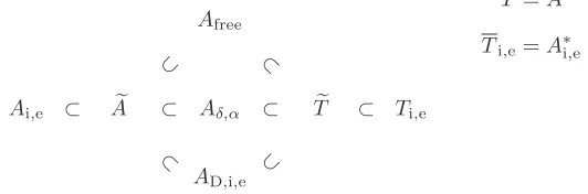
[image:18.612.174.440.495.583.2]e T =Ae∗ Ti,e=A∗i,e
Figure 1. This figure shows how the operatorAδ,α is related to the other operators studied in this section. The operators Afree, Aδ,αandAD,i,e are self-adjoint.
Birman–Schwinger principle; it coincides with the one in [18]. The first item of Theorem3.5is part of Theorem A in the introduction.
Theorem 3.5. LetAδ,αbe as above and letAfreebe the self-adjoint operator defined in (3.5). LeteγandMfbe theγ-field and the Weyl function associated with the quasi boundary triple Πe from Proposition 3.2. Then the following statements hold.
(i) The operatorAδ,αis self-adjoint in the Hilbert space L2(Rn). (ii) For allλ∈ρ(Aδ,α)∩ρ(Afree)the following Krein formula holds:
(Aδ,α−λ)−1−(Afree−λ)−1=eγ(λ) I−αMf(λ)−1αeγ(λ)∗,
where(I−αMf(λ))−1∈ B(L2(Σ)). (iii) For allλ∈R\σ(Afree)we have
λ∈σp(Aδ,α) ⇐⇒ 0∈σp I−αfM(λ)
anddim ker(Aδ,α−λ) = dim ker(I−αfM(λ)).
Proof. Under our assumptions on the function α the operator of multiplication with αis bounded and self-adjoint in the Hilbert spaceL2(Σ). The values of the Weyl function Mfare compact operators in L2(Σ); see Proposition3.2(iii). Now the assertions (i)–(iii) follow from Theorem2.8.
The next theorem gives assumptions onα, which ensure that the domain of the self-adjoint operatorAδ,αhasH2-regularity inRn\Σ. This theorem is the first part of Theorem B in the introduction. Recall thatW1,∞(Σ) is the Soboloev space of order one ofL∞functions on Σ; cf. Section 2.3.
Theorem 3.6. Let Aδ,α be the self-adjoint Schr¨odinger operator in Definition3.4 and assume, in addition, that the function α: Σ →R belongs toW1,∞(Σ). Then domAδ,α is contained inH2(Rn\Σ).
Proof. For any function f ∈ domAδ,α we have f ∈domTe⊂ H∆3/2(Rn\Σ). Then by Proposition3.2(i)
e
Γ1f ∈H1(Σ).
The definition of the operatorAδ,α, the assumptions on the smoothness ofαand the property (2.17) imply that
(3.14) eΓ0f =αeΓ1f ∈H1(Σ). Let us fixλ∈C\R. By the standard decomposition (3.15) domTe= domAfree∔ker(Te−λ)
the function f ∈ domAδ,α can be represented in the form f =ffree+fλ, where ffree∈domAfree andfλ∈ker(Te−λ). It is clear that
ffree∈H2(Rn)⊂H2(Rn\Σ). Relation (3.14) andAfree=Te↾kereΓ0 yield
The properties of the trace map in (2.18) show that Γ0e maps the space domTe∩
H2(Rn\Σ) ontoH1/2(Σ), and hence (3.15) implies thateΓ0 maps ker(Te−λ)∩H2(Rn\Σ)
bijectively ontoH1/2(Σ). This observation and (3.16) show fλ ∈H2(Rn\Σ), and
thereforef =ffree+fλ∈H2(Rn\Σ).
It follows from the proof that for Theorem 3.6 to hold it is sufficient that the multiplication byαmapsH1(Σ)-functions intoH1/2(Σ).
A common method to define self-adjoint Schr¨odinger operators withδ-interactions on hypersurfaces makes use of semi-bounded closed sesquilinear forms. For this consider the sesquilinear form
(3.17) aδ,α[f, g] = ∇f,∇g+ V f, g− αf|Σ, g|ΣΣ, f, g∈H1(Rn). As it is shown in [18], for a real-valuedα∈L∞(Σ) and a real-valuedV ∈L∞(Rn), the form aδ,α is semi-bounded, closed and symmetric. The first representation theorem — see [56, Theorem VI.2.1] or [64, Theorem VIII.15] — yields that a unique self-adjoint operator Aδ,α in L2(Rn) corresponds to the form aδ,α in the sense that
(Aδ,αf, g) =aδ,α[f, g] for allf ∈domAδ,αandg∈domaδ,α=H1(Rn). In the next proposition we show that our approach leads to the same operator.
Proposition 3.7. The self-adjoint Schr¨odinger operator Aδ,α in Definition 3.4 and the self-adjoint operator Aδ,αcorresponding to the sesquilinear form in (3.17)
coincide.
Proof. First we show the inclusion domAδ,α⊂domaδ,α. For this letf =fi⊕fe∈
domAδ,α. According to (3.13) we have, in particular,
fi∈H3/2(Ωi)⊂H1(Ωi), fe∈H3/2(Ωe)⊂H1(Ωe), and fi|
Σ=fe|Σ. Making use of [2, Theorems 5.24 and 5.29] a standard extension argument implies thatf ∈H1(Rn) and hence domAδ,α⊂domaδ,α.
Next letf =fi⊕fe ∈domAδ,α andg =gi⊕ge ∈domaδ,α. Thenaδ,α[f, g] is well defined. By the first Green’s identity (2.20) we have
(∇fi,∇gi)i−(∂νifi|Σ, gi|Σ)Σ= (−∆fi, gi)i,
(∇fe,∇ge)e−(∂νefe|Σ, ge|Σ)Σ= (−∆fe, ge)e.
Using this and the relationαf|Σ=∂νefe|Σ+∂νifi|Σwe obtain
aδ,α[f, g] = (∇f,∇g) + (V f, g)− αf|Σ, g|ΣΣ = (∇fi,∇gi)i+ (∇fe,∇ge)e+ (V f, g)− ∂νifi|Σ, gi|Σ
Σ− ∂νefe|Σ, ge|Σ
Σ
= (−∆fi, gi)i+ (−∆fe, ge)e+ (V f, g) = (−∆ +V)f, g.
Now the first representation theorem (see [56, Theorem VI.2.1]) implies that f ∈
3.3. Schr¨odinger operators with δ′-interactions on hypersurfaces:
self-adjointness, Krein’s formula andH2-regularity. In this section we make use of quasi boundary triples to define and study the Schr¨odinger operator Aδ′,β as-sociated with the formal differential expression Lδ,α = −∆ +V −βhδΣ′,· iδ′Σ in (1.1). The methodology and presentation is very much the same as in the previous section. We mention that to the best of our knowledge a systematic treatment of δ′-potentials on hypersurfaces is not contained elsewhere; see the list of open problems in [30].
In analogy to (3.7) and (3.8) we define the symmetric extension
(3.18) Ab:=Afree∩AN,i,e=L↾f ∈H2(Rn) :∂νifi|Σ=∂νefe|Σ= 0
of the orthogonal sum Ai,e, defined in (3.2), which will serve as the underlying symmetric operator for the quasi boundary triple in the next proposition, and the operator
(3.19) Tb:=Ti,e↾fi⊕fe∈H∆3/2(Rn\Σ) :∂νefe|Σ+∂νifi|Σ= 0 .
We remark that the quasi boundary triple and Weyl function below appear also implicitly in [66, Section 4] in a different context.
Proposition 3.8. Let the operators Ab,Tb,AD,i,e,AN,i,e andAfree be as in (3.18),
(3.19),(3.3),(3.4)and (3.5), respectively, and letMiandMe be the Weyl functions from Proposition 3.1. Then the following statements hold.
(i) The tripleΠ =b {L2(Σ),bΓ0,Γ1b }, where b
Γ0f =∂νefe|Σ, bΓ1f =fe|Σ−fi|Σ, f =fi⊕fe∈domT ,b
is a quasi boundary triple for Ab∗. The restrictions of Tb to the kernels of
the boundary mappings are
b
T ↾kerΓ0b =AN,i,e and Tb↾kerbΓ1=Afree,
and the ranges of the boundary mappings are
ranbΓ0=L2(Σ) and ranbΓ1=H1(Σ). (ii) For λ∈ρ(AN,i,e)andϕ∈L2(Σ) the problem
(L −λ)f = 0, ∂νefe|Σ=−∂νifi|Σ=ϕ,
has the unique solution bγ(λ)ϕ∈H∆3/2(Rn\Σ), where bγ is the γ-field
asso-ciated with Πb. Moreover, bγ(λ)is bounded fromL2(Σ) toL2(Rn).
(iii) For λ ∈ ρ(AN,i,e) the values Mc(λ) of the Weyl function associated with
b
Π are bounded operators from L2(Σ) to H1(Σ) and compact operators in L2(Σ). If, in addition, λ ∈ ρ(Afree), then Mc(λ) is a bijective map from
L2(Σ) ontoH1(Σ). Moreover, the identity (3.20) Mc(λ) =Mi(λ) +Me(λ)
holds for allλ∈ρ(AN,i,e).
χ ∈ C∞
0 (Rn) as in the proof of Proposition3.2, i.e. such that χ ≡1 on an open neighbourhood of Ωi. Let DL be the double-layer potential associated with the hypersurface Σ and the differential expression−∆ + 1; see, e.g. [62, Section 6] for the discussion of double-layer potentials. By [62, Theorem 6.11, Theorem 6.12 (ii)] for an arbitraryϕ∈H1(Σ) the functionf :=χDLϕbelongs to domTband satisfies the condition
fe|Σ−fi|Σ=ϕ, henceΓ1fb =ϕ, and thus ranΓ1b =H1(Σ).
(ii)–(iii) The properties of the γ-field bγ and the Weyl function Mcfollow from Proposition2.7in the same way as in the proof of Proposition3.2(ii)–(iii). We only verify the identity (3.20). For this let λ∈ρ(AN,i,e), so that the operatorsMi(λ), Me(λ) and Mc(λ) all exist; cf. Proposition3.1. IfMc(λ)ϕ=ψ for someϕ∈L2(Σ) andψ∈H1(Σ), then there existsf =fi⊕fe∈ker(Tb−λ) such that
b
Γ0f =ϕ and bΓ1f =ψ. Asfi ∈ker(Ti−λ) andfe∈ker(Te−λ), we have
Γ1,ifi=Mi(λ)Γ0,ifi =−Mi(λ)ϕ, Γ1,efe=Me(λ)Γ0,efe=Me(λ)ϕ, and hence
c
M(λ)ϕ=fe|Σ−fi|Σ=Me(λ)ϕ+Mi(λ)ϕ.
Since this is true for arbitraryϕ∈L2(Σ), relation (3.20) follows.
Remark 3.9. Assume for simplicity that the potentialV in the differential expres-sionLin (3.1) is identically equal to zero. Note that the problem in (ii) is decoupled into an interior and an exterior problem. Let, as in Remark3.3,Gλbe the integral kernel of the resolvent ofAfree. Then for allψ∈C∞(Σ)
b
γ(λ)Mc(λ)−1ψ(x) = Z
Σ
∂νi(y)Gλ(x, y)
ψ(y)dσy, x∈Rn\Σ,
and
c
M(λ)−1ψ(x) =−∂νi(x)
Z
Σ
∂νi(y)Gλ(x, y)
ψ(y)dσy, x∈Σ,
where ∂νi(x) and ∂νi(y) are the normal derivatives with respect to the first and
second arguments with normals pointing outwards of Ωi, and σy is the natural Lebesgue measure on Σ. Note that the operatorbγ(λ)Mc(λ)−1 is, roughly speaking, an extension of the acoustic double-layer potential for the Helmholtz equation, see, e.g. [62, Chapter 6]. The representation of Mc(λ)−1, given above, appears also in [66] in a slightly different context.
We repeat the definition of the Schr¨odinger operator withδ′-potential from the introduction and relate it to the quasi boundary tripleΠ.b
Definition 3.10. For a real-valued functionβsuch that 1/β∈L∞(Σ) the Schr¨odinger operator withδ′-potential on the hypersurface Σ and strengthβ is defined as fol-lows:
which is equivalent to
Aδ′,βf :=−∆f+V f,
domAδ′,β:= (
f ∈H∆3/2(Rn\Σ) : ∂νefe|Σ=−∂νifi|Σ
β∂νefe|Σ=fe|Σ−fi|Σ
) . (3.21)
The definition ofAδ′,β is compatible with the definition of a pointδ′-interaction in the one-dimensional case [3, Section I.4], [4] and the definition of the operator withδ′-potentials on spheres given in [6,68]. Note that, in contrast to the domain ofAδ,α, the domain of Aδ′,β is not contained inH1(Rn).
AN,i,e
⊂
Ai,e ⊂ Ab ⊂ ⊂
⊂
Aδ′,β ⊂ Tb ⊂ Ti,e
Afree ⊂
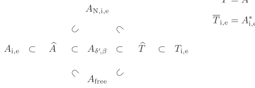
[image:23.612.174.435.255.345.2]b T =Ab∗ Ti,e=A∗i,e
Figure 2. This figure shows how the operatorAδ′,β is related to the other operators studied in this section. The operatorsAN,i,e, Aδ′,β and Afreeare self-adjoint.
The next theorem is the counterpart of Theorem3.5 and can be proved in the same way. Theorem3.11shows the self-adjointness ofAδ′,β and provides a factor-ization for the resolvent difference of Aδ′,β and AN,i,e via Krein’s formula and a variant of the Birman–Schwinger principle. The first item of the next theorem is part of Theorem A in the introduction.
Theorem 3.11. Let Aδ′,β be as above and let AN,i,e be the self-adjoint operator
defined in (3.4). LetbγandMcbe theγ-field and the Weyl function associated with the quasi boundary triple Πb from Proposition 3.8. Then the following statements hold.
(i) The operatorAδ′,β is self-adjoint in the Hilbert space L2(Rn). (ii) For allλ∈ρ(Aδ′,β)∩ρ(AN,i,e)the following Krein formula holds:
(Aδ′,β−λ)−1−(AN,i,e−λ)−1=bγ(λ) I−β−1Mc(λ) −1
β−1γ(λ)b ∗,
where(I−β−1Mc(λ))−1∈ B(L2(Σ)). (iii) For allλ∈R\σ(AN,i,e)we have
λ∈σp(Aδ′,β) ⇐⇒ 0∈σp I−β−1Mc(λ)
anddim ker(Aδ′,β−λ) = dim ker(I−β−1Mc(λ)).
Theorem 3.12. LetAδ′,βbe the self-adjoint Schr¨odinger operator in Definition3.10
and assume, in addition, that the functionβ: Σ→Ris such that1/β∈W1,∞(Σ).
Then domAδ′,β is contained inH2(Rn\Σ).
Proof. The proof proceeds as the proof of Theorem3.6withAδ,α,Afree,Te,eΓ0,eΓ1 and α replaced by Aδ′,β, AN,i,e, T,b Γ0,b bΓ1 and β−1, respectively. Instead of the decomposition (3.15) one has to use the decomposition
domTb= domAN,i,e∔ker(Tb−λ), λ∈C\R.
3.4. Semi-boundedness and point spectra. In this section we show that the self-adjoint operatorsAδ,αandAδ′,β are lower semi-bounded, and that in the case V ≡0 their negative spectra are finite. We recall some preparatory facts on semi-bounded quadratic forms first.
Definition 3.13. For a (not necessarily closed or semi-bounded) quadratic formq in a Hilbert spaceHwe definethe number of negative squares κ−(q) by
κ−(q) := supdimF:F linear subspace of domq
such that∀f ∈F\ {0}:q[f]<0 . Assume that A is a (not necessarily semi-bounded) self-adjoint operator in a Hilbert spaceHwith the corresponding spectral measureEA(·). Define the possibly non-closed quadratic formsA by
sA[f] := (Af, f)H, domsA:= domA.
If, in addition, A is semi-bounded, then by [56, Theorem VI.1.27] the form sA is closable, and we denote its closure by sA. According to the spectral theorem for self-adjoint operators and [15, 10.2 Theorem 3]
(3.22) dim ranEA(−∞,0) =κ−(sA) =κ−(sA).
In particular, ifκ−(sA) is finite, then the self-adjoint operatorAhas finitely many negative eigenvalues with finite multiplicities.
In the caseV ≡0 we write−∆δ,α,−∆δ′,β and−∆freeinstead ofAδ,α,Aδ′,β and Afree. Now we are ready to formulate and prove the main results of this section. The next theorem is part of Theorem A in the introduction. We mention that finiteness of the negative spectrum in the case ofδ-potentials on hypersurfaces was also shown in [18] by other methods.
Theorem 3.14. Let α, β: Σ → R be such that α,1/β ∈L∞(Σ) and let the
self-adjoint operators −∆δ,α and −∆δ′,β be as above. Then the following statements
hold.
(i) σess(−∆δ,α) =σess(−∆δ′,β) = [0,∞).
(ii) The self-adjoint operators −∆δ,α and −∆δ′,β have finitely many negative
eigenvalues with finite multiplicities.
Proof. (i) According to Theorem 4.3in Section 4.2below the resolvent difference of the self-adjoint operators−∆δ,αand−∆free is compact; thus
Analogously, according to Theorem4.5 below the resolvent difference of the self-adjoint operators−∆δ′,β and−∆free is also compact. Hence
σess(−∆δ′,β) =σess(−∆free) = [0,∞). (ii) Let us introduce the (in general non-closed) quadratic forms
s−∆δ,α[f] := −∆δ,αf, f
, dom(s−∆δ,α) := dom(−∆δ,α),
s−∆δ′,β[f] := −∆δ′,βf, f
, dom(s−∆δ′,β) := dom(−∆δ′,β).
Applying the first Green’s identity (2.20) to these expressions and taking the def-initions (3.13), (3.21) of the domains of the operators−∆δ,α,−∆δ′,β into account we obtain
s−∆δ,α[f] = −∆fi, fi
i+ −∆fe, fe
e
= ∇fi,∇fii− ∂νifi|Σ, fi|Σ
Σ+ ∇fe,∇fe
e− ∂νefe|Σ, fe|Σ
Σ
= ∇f,∇f− αf|Σ, f|ΣΣ and
s−∆δ′,β[f] = −∆fi, fi
i+ −∆fe, fe
e
= ∇fi,∇fii− ∂νifi|Σ, fi|Σ
Σ+ ∇fe,∇fe
e− ∂νefe|Σ, fe|Σ
Σ
= (∇f,∇f)+ β−1(fe|Σ−fi|Σ), fi|ΣΣ− β−1(fe|Σ−fi|Σ), fe|ΣΣ = ∇f,∇f− β−1(fe|Σ−fi|Σ), fe|Σ−fi|ΣΣ.
For a bounded functionσ: Σ→Rdefine the quadratic formqσ qσ[f] := ∇f,∇f− σfi|Σ, fi|ΣΣ− σfe|Σ, fe|ΣΣ, domqσ:=H1(Rn\Σ).
It follows from [12, Theorem 6.9] (cf. the proof of Proposition3.15below) that the formqσis closed and semi-bounded, and the self-adjoint operator corresponding to qσ has finitely many negative eigenvalues with finite multiplicities. Thus, by (3.22), we haveκ−(qσ)<∞. It can easily be checked that
dom(s−∆δ,α)⊂dom(q|α|/2) and ∀f ∈dom(s−∆δ,α) :s−∆δ,α[f]≥q|α|/2[f].
Using the inequality|a−b|2≤2(|a|2+|b|2) for complex numbersa, bwe obtain dom(s−∆δ′,β)⊂dom(q2/|β|) and ∀f ∈dom(s−∆δ′,β) :s−∆δ′,β[f]≥q2/|β|[f].
These observations yield that
κ−(s−∆δ,α)≤κ−(q|α|/2)<∞ and κ−(s−∆δ′,β)≤κ−(q2/|β|)<∞.
From this and (3.22) it follows that the negative spectra of−∆δ,αand−∆δ′,β are
finite.
In the following proposition the (closed) sesquilinear formt−∆δ′,β which induces
the self-adjoint operator−∆δ′,β is determined. This was posed as an open problem in [30, 7.2]. Note that, by the first representation theorem,t−∆δ′,β is the closure of
the form