Symbolic and Analytic Techniques for Resource
Analysis of Java Bytecode
David Aspinall1, Robert Atkey2, Kenneth MacKenzie1and Donald Sannella1 1
School of Informatics, The University of Edinburgh, Edinburgh 2
Computer and Information Sciences, University of Strathclyde, Glasgow
Abstract. Recent work in resource analysis has translated the idea of amortised resource analysis to imperative languages using a program logic that allows mixing of assertions about heap shapes, in the tradition of separation logic, and assertions about consumable resources. Sepa-rately, polyhedral methods have been used to calculate bounds on num-bers of iterations in loop-based programs. We are attempting to combine these ideas to deal with Java programs involving both data structures and loops, focusing on the bytecode level rather than on source code.
1
Introduction
The ability to move code and other active content smoothly between execution sites is a key element of modern computing platforms. However, it presents huge security challenges, aggravating existing security problems and presenting altogether new ones. One challenging security issue in this context is control of resources (space, time, etc.), particularly on small devices, where computational power and memory are very limited.
A promising approach to security is proof-carrying code [31], whereby mo-bile code is equipped with an independently verifiable certificate consisting of a condensed proof of its security properties. A major advantage of this approach is that it sidesteps the difficult issue of trust: there is no need to trust either the code producer, or a centralized certification authority. Work on the PCC approach to resource security includes [35] and [7].
Recent developments in static analysis methods now makes it feasible to consider an alternative but related approach to security. Instead of requiring the code producer to supply a proof, whether via static analysis of source code or by other means, one can perform an analogous analysis directly on the down-loadable bytecode to determine its properties. This could be done by the code consumer on receipt of downloadable code, dispensing with the need for a proof. Alternatively, the code producer could perform the analysis and use the result to produce a proof certificate. An interesting third alternative is that an in-termediary, for example a software distributor, could perform such an analysis on uncertified bytecode, transforming it to proof-carrying code. The fact that the original source code is not required is essential to making this feasible in commercial practice.
Here we consider two quite different approaches to the analysis of resource consumption of Java bytecode. The first, in§2, translates the idea of amortised resource analysis to imperative languages to enable automated resource analysis of programs that iterate through data structures. The second, in§3, uses poly-hedral methods to calculate resource bounds of iterative procedures controlled by numerical quantities. In §4 we briefly describe some ideas for future work and plans for integrating the two kinds of analysis to deal with Java programs involving both data structures and loops.
2
Amortised Resource Analysis
Amortised resource analysis is a technique for specifying and verifying resource bounds of programs by exploiting the tight link between the structure of the data that programs manipulate and the resources they consume. For instance, a program that iterates through a list doing something for every element can either be thought of as requiring n resources, where n is the length of list, or as requiring 1 resource for every element of the list, where we never know the global length property of the list. Taking the latter view can simplify both the specification and the verification of programs’ resource usage.
This work conceptually builds on the work of Tarjan and Sleator on amor-tised complexity analysis [36], where “credits” and “debits” may be virtually stored within data structures and used to pay for expensive operations. By stor-ing up credit for future operations in a data structure, we amortise the cost of operations on the data structure over time. Hofmann and Jost [21] applied this technique to first-order functional programs to yield an automated resource analysis. Atkey [3] has recently adapted this work to integrate with Separation Logic [22, 34] to extend the automated technique to pointer-manipulating imper-ative programs. In this section we give an overview of Atkey’s work and describe some examples.
2.1 Integrating the Banker’s Method and Separation Logic
makeAtrue andBtrue respectively. Resource separation enables local reasoning about mutation of resources; if the program mutates the resource associated with A, then we know thatB is still true on its separate resource.
For the purposes of complexity analysis, we want to consider resource con-sumption as well as resource mutation, e.g. the concon-sumption of time as a program executes. To see how Separation Logic-style reasoning about resources helps in this case, consider the standard inductively defined list predicate from Separa-tion Logic, augmented with an addiSepara-tional proposiSepara-tion R denoting the presence of a consumable resource for every element of the list:
listR(x)≡ x=null∧emp
∨ ∃y, z.[xdata7→ y]∗[xnext7→ z]∗R∗listR(z)
See Atkey [3] for a complete description of the assertion logic. We can represent a heapH and a consumable resourcerthat satisfy this predicate graphically:
H
r
null a
R
b
R
c
R
d
R
So we have r, H |= listR(x), assuming x points to the head of the list. Here r = R·R·R·R—we assume that consumable resources form a commutative monoid—and rrepresents the resource that is available for the program to use in the future. We can splitH andrto separate out the head of the list with its associated resource:
H1
r1
H2
r2
null a
R
b
R
c
R
d
R
This heap and resource satisfyr1·r2, H1]H2|= [x data
7→ a]∗[xnext7→ y]∗R∗listR(y), whereH1]H2=H,r1·r2=rand we assume thatypoints to thebelement. Now that we have separated out the head of the list and its associated consumable resource, we are free to mutate the heapH1and consume the resourcer1without affecting the tail of the list, so the program can move to a state:
H1 H2
r2
null
A b
R
c
R
d
R
The combined assertion about heap and consumable resource describes the current shape and contents of the heap and also the available resource that the program may consume in the future. By ensuring that, for every state in the program’s execution, the resource consumed plus the resource available for consumption in the future is less than or equal to a predefined bound, we can ensure that the entire execution is resource bounded.
Intermixing resource assertions with Separation Logic assertions about the shapes of data structures, as we have done with the resource-carryinglistR pred-icate above, allow us to specify amounts of resource that depend on the shape of data structures in memory. By the definition oflistR, we know that the amount of resource available to the program is proportional to the length of the list, with-out having to do any arithmetic reasoning abwith-out lengths of lists. The association of resources with parts of a data structure is exactly the banker’s approach to amortised complexity analysis proposed by Tarjan [36].
In the exposition above we have used a list predicatelistR(x) that describes a list on the heap with a fixed number of resources per element. Using this predicate only allows the specification of resource usage that is linear in the lengths of lists. Recent work by Hoffmann and Hofmann [20] on amortised resource analysis for polynomial bounds lifts this restriction. Preliminary experiments with combining the two techniques have been promising.
2.2 Implementation
The combination of Separation Logic and amortised resource analysis has been implemented in two stages. We have formalised and mechanically checked a proof of soundness for the combined program logic for a simplified subset of Java bytecode in Coq with a shallowly embedded assertion logic. On top of this we have implemented a Coq-verified verification condition generator for a deeply embedded assertion logic and extracted this to OCaml. In OCaml we have implemented a proof search procedure that solves verification conditions using a similar technique to other automated verification tools for Separation Logic [11]. See Atkey [3] for more details. In our proof search implementation, we can leave resource annotations, e.g. the resource associated with each element of a list, as variables to be filled in by a linear program solver. Our tool requires annotation of programs with loop invariants, but can infer the resource portion. This process is demonstrated in the next section.
2.3 A More Complex Example
heap-shape behaviour of the program; the resource bounds simply drop out of shape constraints thanks to the inference of resource annotations.
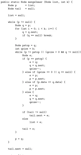
Consider the Java method declaration shown in Figure 13 that describes the inner loop of an in-place merge sort algorithm for linked lists. The method takes two arguments: list, a reference to the head node of a linked list; and k, an integer. The integer argument dictates the sizes of the sublists that the method will be merging in this pass. In short, the method steps through the list 2*k
elements at a time, merging the two lengthksublists each time. The outer loop does the2*kstepping, and the inner loop does the merging. To accomplish a full merge sort, this method would be called log2(n) times with doublingk, wheren is the length of the list.
Assume that we wish to account for the number of swapping operations per-formed by this method, i.e. the number of times that the third branch of theif
statement in the inner loop is executed. We accomplish this in our implementa-tion by inserting a specialconsumeinstruction at this point.
The pre- and post-conditions of the method are as follows:
Pre(mergeInner) :list6=null∧(lseg(x,list,null)∗Ry)
Post(mergeInner) :lseg(0,retval,null)
The precondition states that the first argument points to a list segment ending withnull, withxamount of resource associated with every element of the list, andyamount of additional resource that may be used. The values ofxandywill be inferred by a linear program solver. The condition list 6=null is a safety condition required for the method to not throw a null pointer exception.
The outer loop in the method needs a disjunctive invariant corresponding to whether this is the first iteration or a later iteration.
(lseg(o1,list,tail)∗[tail next
7→?]∗[taildata7→?]∗lseg(o2,p,null)∗Ro3) ∨((list=null∧tail=null)∗lseg(o4,p,null)∗Ro5)
The first disjunct is used on normal iterations of loop: the variablelistpoints to the list that has been processed so far, ending attail;ppoints to the remainder of the list that is to be processed. We have annotated these lists with the resource variableso1 ando2that will contain the resources associated with each element of these lists. The second disjunct covers the case of the first iteration, when
list andtailare null andppoints to the complete list to be processed. Moving on, we consider the first inner loop that advances the pointerqbyk
elements forward, thus splitting the list ahead ofpinto ak-element segment and the rest of the list. The next loop will merge the firstk-length segment with the
k-length prefix of the second segment. It is convenient for our implementation to split out this inner loop into another method4, with the following signature:
3 Adapted from the C code at
http://www.chiark.greenend.org.uk/~sgtatham/algorithms/listsort.html. 4 This is because our implementation works on unstructured bytecode, and so cannot
public static Node mergeInner (Node list, int k) { Node p = list;
Node tail = null;
list = null;
while (p != null) { Node q = p;
for (int i = 0; i < k; i++) { q = q.next;
if (q == null) break; }
Node pstop = q; int qsize = k;
while (p != pstop || (qsize > 0 && q != null)) { Node e;
if (p == pstop) { e = q; q = q.next; qsize--;
} else if (qsize == 0 || q == null) { e = p;
p = p.next;
} else if (p.data <= q.data) { e = p;
p = p.next; } else {
e = q; q = q.next; qsize--; }
if (tail != null) tail.next = e; else
list = e;
tail = e; }
p = q; }
tail.next = null;
[image:6.612.132.398.113.622.2]return list; }
public static Node advance (Node l, int k)
The argumentlpoints to a linked list, and the method will advancekelements through the list (or until the end) and return a pointer to the split point. The pre- and post-condition of this method are:
Pre(advance) :lseg(a0,l,null)
Post(advance) :lseg(a0,l,retval)∗lseg(a0,retval,null)
Again, we have left the resource annotation on the elements of the list as a variable a0, to be filled in by the linear solver. The appearance of the same variable in the pre- and post-condition implies that we expect this resource to be preserved by the method.
Proceeding though our main method, the invariant of the inner loop is as follows, again in two pieces according to whether it is the first or second iteration of the outer loop:
(lseg(i1,list,tail)∗[tail next
7→?]∗[taildata7→?]
∗ lseg(i2,p,pstop)∗lseg(i3,q,null)∗Ri4)
∨((list=null∧tail=null)∗lseg(i5,p,pstop)∗lseg(i6,q,null)∗Ri7) The first part of each disjunct is as before, stating that list totail contains the part of list that has been processed. Since we have now split the remainder of the list into two pieces we have two separate list segments referenced bypand
qpointing to the parts of the list that are to be merged.
Running this example through our implementation produces the solution x= 1,y= 0 for the precondition resource annotations. This indicates that each element of the list needs to contain one resource for every element. For the outer loop’s invariant, we obtain o2 =o4 = 1 and all the others are 0. This indicates that the list we have processed has had all its resources consumed, while the list remaining to be processed still has associated resources. This is as expected for a loop iterating through a list. The specification ofadvanceis completed by inferringa0= 1, indicating thatadvancepreserves the resources associated with the list. Finally the inner loop’s invariant hasi2=i3=i5=i6= 1 and all others 0, indicating that the two list segments that are remaining to be processed have associated resources, while the processed segments do not.
Comparisons to other techniques. While we have had to work to supply the loop invariants for our implementation, we note that these invariants may be inferred by other tools, for example [11], and the resource variables automatically inserted on the list segment parts. The key to the amortised approach is the tight connection between shape invariants, which is a complex but well-studied problem, and resource usage.
structures, but only via abstract interfaces. The specifications for these abstract interfaces record the effect of the operations on the size of the data structure. Thus, the technique is unable to cope with the kind of program that we have presented above that uses direct pointer manipulation. Nevertheless, Gulwani et al report impressive results on real-world Microsoft product code.
The COSTA system [2] can deal with some uses of direct pointer manipula-tion, but accounts for the sizes of heap-based data structures by counting the length of the longest path from a given reference. Thus, it cannot deal with pro-grams that demonstrate sharing on the heap; the Java method described above has three pointers all pointing the same list in the inner loop.
One might also consider the use of Separation Logic to deal with sharing on the heap, augmented with information on the sizes of heap-base data structures to account for resource usage. So one would have a predicate lsegn(x, y) that describes a list segment of length n from x to y, plus a “ghost variable” that accounts for the consumed resources. We argue that the amortised approach described here is simpler due to the differences in reasoning between the global property of the length of a whole list, and thelocal property of each list element having an associated amount of resource to be used. For example, consider the specification of theadvancemethod using sized structures:
Pre(advance) :lsegn(l,null)
Post(advance) :∃n1, n2. n1+n2=n∧(lsegn1(l,retval)∗lsegn2(retval,null)) We have had to introduce two existential variables indicating the sizes of the lists returned by the method. These additional values have to then be related back to the length of the original list by the calling method, and thence to the resource consumption, requiring non-straightforward arithmetic reasoning. The amortised approach exploits the shape-reasoning already present in Sepa-ration Logic to account for resources. For further elaboSepa-ration of this point, and a demonstration of the use of amortised specification to improve information hiding in specifications, see the functional queues example in [3].
3
Iteration and geometry
The previous section has described a technique which can be used to analyse the resource usage of procedures which manipulate heap-based data structures. Here we will describe a mathematical technique which can be used to study iterative procedures controlled bynumericalquantities. One of our main interests is in producingcertifying analyses, and our description of the mathematics will highlight aspects which are relevant to this problem.
We will look at some examples of Java methods which use iteration. For simplicity, we will look at the problem of deciding how often theprintlnmethod is called, but we could equally be looking at object allocation or the transmission of SMS messages.
public static void m1() { for (int i=1; i<=9; i++)
for (int j=1; j<=i && j<=7; j++) System.out.println ("Hello"); }
For a more complicated example, consider this Java method where both loops are controlled by method arguments:
public static void m2 (int p, int q) { for (int i=0; i<=p; j++)
for (int j=0; j<=9 && i+j<=q; j++) System.out.println ("Hello"); }
How can one tell how many timesprintlnis called in these methods? Consider
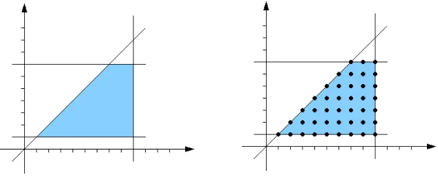
m1 again. Every time we visit the println statement we have the following constraints on the program variablesiandj:
1≤i≤9
1≤j≤i
1≤j≤7.
Considered as inequalities over the real numbers, these define a trapezoidal region P in the (i, j)-plane, and it is easy to see that the number of times theprintln
statement is executed is equal to|P∩Z2|, the number of lattice points5within the polygonP.
Fig. 2.PolygonP for methodm1 Fig. 3.Lattice points inP
There is a rich mathematical theory of the enumeration of lattice points in polytopes (the generalisation of polygons to higher dimensions) and we will describe some aspects of this theory and its relations to program analysis.
5
[image:9.612.151.468.441.576.2]3.1 Halfspaces, polyhedra, and polytopes
Fix an integer d ≥ 0 and a1, . . . , ad ∈ R. We will be interested in solutions (x1, . . . , xn)∈Rd of inequalities of the form
a1x1+· · ·+adxd ≤b. (1)
In our applications, such inequalities will arise in the form of linear constraints on program variables. Putting a = (a1, . . . , ad) and x = (x1, . . . , xd) we can
rewrite (1) asa·x≤b, and if a6=0then the set ofx satisfying the inequality defines a halfspace in Rd. For example, in R2 a halfspace consists of all points lying on one side of some line.
Aconvex polyhedroninRdis the intersection of a finite number of halfspaces, and a bounded polyhedron (a polyhedron of finite extent, i.e. one which is con-tained in some sphere) is called a polytope. It can be shown that a polytope can equivalently be defined as the convex hull6 of a finite set of points in Rd (theverticesofP). Moreover, if the constants in the inequalities definingP are all rational (as will be the case in all of our applications), the vertices of P all have rational co-ordinates. A convex polyhedron is thus the set of simultaneous solutions to a system ofninequalities:
a11x1+· · ·+a1dxd≤b1 a21x1+· · ·+a2dxd≤b2
.. .
an1x1+· · ·+andxd≤bn.
The general theory of polyhedra has many applications in mathematics and in computer science. See [6] for a survey of applications in computer science.
Note that if we restrict to natural numbers, then linear inequalities of the type considered above are exactly the type of inequalities that occur in Presburger arithmetic. It follows that the lattice point enumeration problem subsumes the problem of counting solutions to systems of Presburger inequalities. This point of view is examined in greater depth by Pugh in [33].
3.2 Ehrhart Polynomials
Many applications of polytope methods have been based on the work of Eug`ene Ehrhart [17, 18], who studied the problem of how the number of lattice points inside a polytope grows as the size of the polytope increases. More precisely, let
P = conv{y1, . . . ,ym}
be a polytope and forn∈N, let
nP = conv{ny1, . . . , nym} 6
be then-fold dilate ofP. Ehrhart showed that|nP∩Zd|is aquasipolynomial in
n, which may be thought of as a number of polynomials cyclically interleaved.
Definition. Aquasipolynomial of degree dis a functionf :Z→Zof the form
f(n) =
f0(n) ifn≡0 (mod k) f1(n) ifn≡1 (mod k)
.. .
fk−1(n) ifn≡k−1 (modk).
where eachfjis a polynomial of the usual kind and max{degf0, . . . ,degfk−1}= d. The (minimal) numberkof polynomial components is called the quasiperiod off.
Theorem. Let P = conv{y1, . . . ,yn} be a rational convex polytope in Zd and let
EP(n) =|nP∩Zd|.
Then EP(n) is a quasipolynomial of degreedimP and quasiperiod equal to the
greatest common denominator of the coordinates of the vertices of P.
The original proof of this theorem can be found in [17]; see also [9, Chapter 3]. There is a considerable amount of research applying Ehrhart polynomials to program analysis and optimisation, especially in the field of high-performance computing involving array calculations. One of the first papers in this area is due to Clauss [14], with application to problems such as counting the flops executed by a loop, the number of memory locations touched by a loop, the array elements that must be transmitted from one processor to another during parallel array computations, the maximum parallelism induced by a loop from a given time-schedule, and several others. Further work appears in [25, 15, 38] for example.
The methods of Clauss seem to have remained largely within the high-performance/parallel computing community (see [24, 32] for example) until 2006, when Braberman et al [13] (and see also [12]) showed how to adapt these tech-niques to predict the memory usage of (iterative) Java programs; at present this appears to be the only application of polytope methods within the programming language community.
3.3 Drawbacks of Ehrhart polynomials
polytopePis the greatest common denominator of the coefficients of the vertices ofP, it becomes clear that a considerable amount of computation can be required to calculateEP(n). In addition to this, the initiald+1 values of thekpolynomial
components of the quasipolynomial have to be computed by explicitly counting the number of lattice points in the dilates 0P, P,2P, . . . ,(d+ 1)P. The number k can be very large, even for relatively simple polytopes. For example, for the triangular polytope
P= conv{(1 4,
2 5),(
5 7,
2 11),(
8 9,
1 12)}
the quasiperiod ofEP(n) is 13,680. Calculating the Ehrhart polynomial ofPthus
requires the solution of 13,680 3×3 systems of linear equations, which would be reasonably time-consuming. In fact, even if the dimensiondis fixed, the time taken to compute (via interpolation) the Ehrhart polynomial of a polytope with n vertices can grow exponentially withn (see [38,§2.3]), whereas the methods presented in the next section are polynomial in fixed dimension.
The sheer amount of data required to specify an Ehrhart function is also something of a barrier in the context of certified resource analysis, where such functions would have to be recorded in certificates accompanying mobile pro-grams. This may not in fact be an insurmountable problem. One could possibly find simpler functions which are upper bounds for the exact Ehrhart function (see [30]); this would save space at the expense of a (hopefully small) loss of pre-cision. Another issue is that Ehrhart functions are not arbitrary quasipolynomi-als: for example it is clear that they are increasing functions, whereas a general quasipolynomial can have polynomial components which are completely unre-lated, leading to a function whose value oscillates drastically. It is conceivable that the quasipolynomials arising as Ehrhart functions have special properties which would enable them to be specified by a relatively small amount of data. Unfortunately, it seems that very little is known about exactly which quasipoly-nomials can occur as Ehrhart polyquasipoly-nomials (see [28, 10] for some partial results) so at present it is difficult to be precise about the minimum of data required to explicitly specify an Ehrhart function. However, the results discussed in the next section may enable us to bypass this problem.
3.4 Generating functions
The difficulty of computing Ehrhart polynomials suggests that they would be unsuitable for polytope-based analyses in a certifying framework, but fortunately some more recent results provide a much more efficient means of enumerating lattice points. The basic tool in this theory is thegenerating function of a poly-tope, which is a multivariate polynomial with a term for every lattice point in the polytope. More concretely, suppose we have a polytope P in Rd. We will
consider polynomials in the variablesx1, . . . , xd. Givenv= (v1, ..., vd)∈Zd we define
xv=xv1
1 x
v2
2 · · ·x
and the generating function of P is then defined by
GP(x) =
X
{xv:v∈P∩Zd}
It is easy to see that the number of lattice points in P is given byGP(1, . . . ,1).
The obvious difficulty here is that the polynomialGP(x) will in general be
enor-mous and costly to compute. Recall our earlier example, which gave rise to a trapezoidal region inR2:
for (i=1; i<=9; i++)
for (j=1; j<=i && j<=7; j++) B
For this relatively small example, the full generating function is
GP(x, y) =xy+x2y+x3y+x4y+x5y+x6y+x7y+x8y+x9y
+x2y2+x3y2+x4y2+x5y2+x6y2+x7y2+x8y2+x9y2
+x3y3+x4y3+x5y3+x6y3+x7y3+x8y3+x9y3
+x4y4+x5y4+x6y4+x7y4+x8y4+x9y4
+x5y5+x6y5+x7y5+x8y5+x9y5
+x6y6+x7y6+x8y6+x9y6
+x7y7+x8y7+x9y7
which is already quite unwieldy.
However, Alexander Barvinok [8] has recently shown how to express the gen-erating function as a sum of short rational functions which are easily determined from local information at the vertices ofP. In the case above, we have
GP(x, y) =
xy
(1−x)(1−xy)+
x9y (1−x−1)(1−y)
+ x
9y7
(1−y−1)(1−x−1)+
x7y7
(1−x)(1−x−1y−1)
This function is easily computed if one knows the vertices and edges of the polytope. Space constraints prevent us from describing the computation in detail here, but a full explanation can be found in [8] or [9].
There is a problem here, though. To find|P∩Z2|we have to evaluateGP(1,1),
and the denominators of all of the terms above vanish at (1,1). However, this can be overcome. The singularity at (1,1) is aremovable singularity[1,§3.1], and various techniques can be used to find lim(x,y)→(1,1)GP(x, y). For example, we
can find a common denominator to obtain
GP(x, y) =
xy−xy2−x10y+x11y2+x10y8−x11y9−x8y8+x8y9 (1−x)(1−y)(1−xy)
= xy−xy
and then repeatedly apply L’Hˆopital’s rule7 to obtain
P∩Z2=GP(1,1)
= lim
(x,y)→(1,1)
xy−xy2−x10y+x11y2+x10y8−x11y9−x8y8+x8y9 1−x−y+x2y+xy2−x2y2
= lim
(x,y)→(1,1)
∂
∂y(xy−xy
2−x10y+x11y2+x10y8−x11y9−x8y8+x8y9)
∂
∂y(1−x−y+x2y+xy2−x2y2)
=· · ·
= −2 + 22 + 560−792−448 + 576 −2
= 42
which is indeed equal to the number of lattice points in Figure 3.
This calculation may appear to be quite complex in relation to our relatively small example, but it is easy to automate8. Note also that the complexity of the calculation depends only on the shape of the polytope, and not its size. If we took a region of a similar shape but many times larger, all that would change would be the exponents ofxandy in the numerator of the generating function; the calculation required to determine the number of lattice points would be essentially identical to that above.
We have only considered Barvinok’s construction for integral polytopes here, but the theory can be extended to rational polytopes as well. it is also possible to recover most of the theory of Ehrhart polynomials, which is useful for the study of parametric bounds. This approach is developed in detail by De Loera et al in [26], which describes the implementation of Barvinok’s techniques in the LattE package. De Loera’s work is applied to program analysis problems in [38], where much of Clauss’ work is recast in terms of Barvinok’s methods. Generating-function methods have recently been applied to the problem of Worst Case Execution Time in [27]. See also [9] for an exposition of the mathematics of the Barvinok theory.
3.5 Implementation
We have implemented (in OCaml) a Java compiler which uses lattice point enu-meration techniques to calculate resource bounds for simple imperative pro-grams. This is a preliminary implementation, but the results it produces are quite promising; it can successfully (and automatically) produce precise bounds for realistic matrix manipulation programs, for example (see Appendix A for some examples).
7 If f and g are continuous at a and lim
x→af(x) = limx→ag(x) = 0 then
limx→af(x)/g(x) = limx→af0(x)/g0(x)
8 The calculation works particularly well for our example because our polygon is
Inferring linear constraints. The first phase of the compiler converts the source program to an expression-based form in which all names have been re-solved. This form is very similar to the source program, and preserves the explicit control-flow structures of Java.
Our first task is to infer systems of linear constraints on program variables. The expression-based form is converted into a control-flow graph and then be-tween every pair of expressions we infer a polyhedron which bounds the values of the integral variables in the program. This is done using a well-known tech-nique due to Cousot and Halbwachs which involves abstract interpretation over a domain of polyhedra. See [16] for details.
A number of polyhedral operations are required to perform this process. It is necessary to have some representation of polyhedra and the means to convert between vertex and facet representations, and methods for combining polyhe-dra in various ways (intersection, join (polyhepolyhe-dral hull), widening, . . . ) are also needed. These can be difficult to program, but fortunately there are a number of high-quality libraries available. We have chosen to use the Parma Polyhedra Library (PPL) [5], which is a large C++ library providing all of the operations we require, including polyhedral widening operators (see [4]) necessary to en-sure termination of the abstract interpretation process. The PPL also provides an OCaml interface which was convenient for linking with our OCaml-based compiler.
Using the PPL it was a relatively straightforward task to implement the Cousot-Halbwachs technique and obtain linear bounds on program variables.
Enumerating lattice points. Having determined polytopes controlling loop iteration, it is necessary to enumerate lattice points in order to find bounds on the number of loop executions. We have done this using thebarvinoklibrary9of Sven Verdoolaege, which implements the generating-function methods described in §3.4, and this enables us to automatically find our desired resource bounds.
There are certain difficulties in this approach however; in particular, it can be difficult to decide which variables control iterations, and what the dimension of the relevant polytope should be. Our prototype compiler works with a repre-sentation which has a fairly explicit reprerepre-sentation of the loop structure of the input program, and we have developed heuristics which enable us to determine the relevant polytopes. This works well in practice, with realistic code examples, but it is possible to devise examples which cause the analysis to give incorrect results. However, we believe that this problem can be solved by methods which will be described below.
3.6 Analysing compiled bytecode
We are currently attempting to apply lattice-point methods to the resource anal-ysis of JVM bytecode methods. A basic problem here is that it can be difficult
9
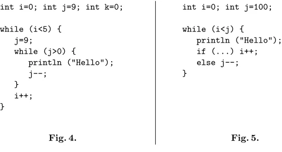
to determine the precise loop structure of a program by examining the bytecode. Consider the following examples.
int i=0; int j=9; int k=0;
while (i<5) { j=9;
while (j>0) {
println ("Hello"); j--;
[image:16.612.149.428.164.314.2]} i++; }
Fig. 4.
int i=0; int j=100;
while (i<j) {
println ("Hello"); if (...) i++; else j--; }
Fig. 5.
In Figure 4, the entire inner loop is executed once for each iteration of the outer loop, and theprintlnmethod is called a total of 45 times; however, if the statement j=9is altered tok=9then the “inner” loop is executed once only, so
printlnis executed only 9 times. This example shows that a very small change (only a single instruction in the compiled bytecode will change) can have a major effect on the resource usage of a program. The two versions of the program even have identical control-flow graphs, so it is not easy to see how to perform an accurate analysis of resource usage.
In Figure 5 the loop is controlled by two variables, but the iteration is one-dimensional. How can we recognise such patterns?
Instrumenting the code with counters. Gulwani et al [19] have proposed a technique for instrumenting withcounter variables which can then be used for resource analysis. The example in Figure 5 would become
int i=0; int j=100; int c=0;
while (i<j) {
println ("Hello"); if (...) {i++; c++;} else {j--; c++} }
The Cousot-Halbwachs technique can successfully analyse this example to deduce that 0 ≤ c ≤ 99, allowing us to conclude that the loop is executed at most 100 times.
dependencies between counters which enable one to attack nested structures such as the one in Figure 4 above. However, the results of the analysis can be somewhat imprecise due to the fact that bounds associated with “nested” counters are simply multiplied together to obtain an overall bound.
We believe that the Gulwani algorithm can be refined to provide more pre-cise relations between counters which can then be analysed using lattice-point methods to give more precise bounds on loop iterations.
We are currently implementing an analysis for compiled JVM bytecode which will combine the instrumentation technique of Gulwani with lattice-point meth-ods and amortised analysis, and we hope that this will allow us to automatically analyse the resource consumption of many programs.
4
Further Work
The lattice-point techniques described above only apply to single methods. We would like to integrate our work with existing techniques to enable analysis of complete Java applications (including recursion).
Some of the geometrical algorithms are computationally expensive; in par-ticular, the complexity of certain polyhedral operations grows exponentially as the dimension increases. We would like to develop certifying versions of these algorithms so that the output can be verified without excessive effort.
Polyhedral libraries are written in C++ and are very large and complex (PPL is over 100,000 lines long), and also depend on a number of external libraries (for example the gmplibrary for unlimited-precision arithmetic). This provides a lot of opportunities for bugs to creep in, and certifying algorithms would have the added benefit that they would allow us to be sure of the correctness of the output without having to trust the correctness of the libraries. See [29, 23] for more on this point of view.
One of our motivations is to measure memory consumption of Java programs. A common assumption in research on this topic is that all objects from a given class are of the same size. However, this will not always be the case: for example, the JavaBigIntegerclass represents integers with unlimited precision, and the size of an object will depend on the integer involved. Furthermore, the size of an object returned by a method may depend on the method arguments — consider theBigInteger multiplymethod. We are not aware of any previous research which is able to deal with this type of behaviour. However, there is some recent work by Verdoolaege and Bruynooghe [37] on weighted generating functions for polytopes, in which instead of considering the usual generating functionP
{xv:v∈P∩
Zd}, one considers a function of the formP{f(v)xv:
v∈P∩Zd}in which each lattice point is weighted according to some functionf.
This corresponds to the situation in which a nest of loops indexed by i1, . . . , id
allocates an amount of memory given by the function f(i1, . . . , id). It seems
Examination of a large number of examples suggests that most methods which involve loops deal either with iteration over data structures or with itera-tion controlled by integer variables, but that it is unusual to encounter situaitera-tions which involve both simultaneously, the most common such situation being the conversion of a list to an array or vice versa. This makes us hopeful that a straightforward combination of our two techniques will enable the automatic analysis of a substantial proportion of Java methods. There are however certain situations where it is difficult to determine the amount of iteration required in advance — for example, worklist algorithms where processing one element of a queue may add an unpredictable number of new elements to the end of the queue, or iterative floating-point numerical algorithms where the number of it-erations required is very sensitive to input data — and these remain beyond the scope of our methods at present.
5
Acknowledgments
This work was funded in part by the Sixth Framework programme of the Euro-pean Community under the MOBIUS project FP6-015905. This report reflects only the author’s views and the European Community is not liable for any use that may be made of the information contained therein.
This work was funded in part by the ReQueST grant (EP/C537068) from the EPSRC e-Science Programme, and by the RESA grant (EP/G006032/1) from the EPSRC Follow-on Fund.
References
1. Lars Ahlfors. Complex Analysis. International Series in Pure and Applied Mathe-matics. McGraw-Hill, 1979.
2. Elvira Albert, Puri Arenas, Samir Genaim, German Puebla, and Damiano Za-nardini. COSTA: Design and implementation of a cost and termination analyzer for Java bytecode. InFormal Methods for Components and Objects, 6th Interna-tional Symposium, FMCO 2007, Revised Lectures, volume 5382 of Lecture Notes in Computer Science, pages 113–132. Springer, 2007.
3. Robert Atkey. Amortised resource analysis with separation logic. InESOP 2010: Proceedings of the 19th European Symposium on Programming Languages and Sys-tems, volume 6012 ofLecture Notes in Computer Science, pages 85–103. Springer, 2010.
4. R. Bagnara, P. M. Hill, E. Ricci, and E. Zaffanella. Precise widening operators for convex polyhedra. Science of Computer Programming, 58(1–2):28–56, 2005. 5. R. Bagnara, P. M. Hill, and E. Zaffanella. The Parma Polyhedra Library: Toward a
complete set of numerical abstractions for the analysis and verification of hardware and software systems. Science of Computer Programming, 72(1–2):3–21, 2008. 6. Roberto Bagnara, Patricia M. Hill, and Enea Zaffanella. Applications of polyhedral
computations to the analysis and verification of hardware and software systems.
7. Gilles Barthe, Lennart Beringer, Pierre Cr´egut, Benjamin Gr´egoire, Martin Hof-mann, Peter M¨uller, Erik Poll, Germ´an Puebla, Ian Stark, and Eric V´etillard. MOBIUS: Mobility, ubiquity, security — objectives and progress report. In Trust-worthy Global Computing: Revised Selected Papers from the Second Symposium TGC 2006, number 4661 in Lecture Notes in Computer Science. Springer-Verlag, 2007.
8. Alexander Barvinok and James E. Pommersheim. An algorithmic theory of lattice points in polyhedra. In New Perspectives in Algebraic Combinatorics (Berkeley, CA, 1996–97), volume 38 ofMath. Sci. Res. Inst. Publ., pages 91–147. Cambridge Univ. Press, 1999.
9. Matthias Beck and Sinai Robins. Computing the Continuous Discretely. Under-graduate Texts in Mathematics. Springer–Verlag, 2007.
10. Matthias Beck, Steven Sam, and Kevin Woods. Maximal periods of (Ehrhart) quasi-polynomials. J. Combin. Theory Ser. A, 115:517–525, 2008.
11. Josh Berdine, Cristiano Calcagno, and Peter W. O’Hearn. Symbolic execution with separation logic. In Kwangkeun Yi, editor, APLAS, volume 3780 ofLecture Notes in Computer Science, pages 52–68. Springer, 2005.
12. V. Braberman, F. Fern´andez, D. Garbervetsky, and S. Yovine. Symbolic prediction of dynamic memory requirements. InISMM 2008, 2008.
13. Victor Braberman, Diego Garbervetsky, and Sergio Yovine. A static analysis for synthesizing parametric specifications of dynamic memory consumption. Journal of Object Technology, 5(5):31–58, Jun 2006.
14. Philippe Clauss. Counting solutions to linear and nonlinear constraints through Ehrhart polynomials: applications to analyze and transform scientific programs. InICS ’96: Proceedings of the 10th International Conference on Supercomputing, pages 278–285, 1996.
15. Philippe Clauss and Vincent Loechner. Parametric analysis of polyhedral iteration spaces. Journal of VLSI Signal Processing, 19:179–194, 1998.
16. Patrick Cousot and Nicolas Halbwachs. Automatic discovery of linear restraints among variables of a program. InPOPL ’78: Proceedings of the 5th Annual ACM Symposium on Principles of Programming Languages, pages 84–97. ACM Press, 1978.
17. Eug`ene Ehrhart. Sur un probl`eme de g´eom´etrie diophantienne lin´eaire. I. Poly`edres et r´eseaux. J. Reine Angew. Math., 226:1–29, 1967.
18. Eug`ene Ehrhart. Sur un probl`eme de g´eom´etrie diophantienne lin´eaire. II. Syst`emes diophantiens lin´eaires. J. Reine Angew. Math., 227:25–49, 1967.
19. Sumit Gulwani, Krishna K. Mehra, and Trishul M. Chilimbi. SPEED: precise and efficient static estimation of program computational complexity. In POPL ’09: Proceedings of the 36th ACM SIGPLAN-SIGACT Symposium on Principles of Programming Languages, pages 127–139, 2009.
20. Jan Hoffmann and Martin Hofmann. Amortized resource analysis with polyno-mial potential. InESOP 2010: Proceedings of the 19th European Symposium on Programming Languages and Systems, volume 6012 ofLecture Notes in Computer Science, pages 287–306. Springer, 2010.
21. Martin Hofmann and Steffen Jost. Static prediction of heap space usage for first-order functional programs. InPOPL ’03: Proceedings of the 30th ACM SIGPLAN-SIGACT Symposium on Principles of Programming Languages, pages 185–197, 2003.
23. Dieter Kratsch, Ross M. McConnell, Kurt Mehlhorn, and Jeremy P. Spinrad. Certi-fying algorithms for recognizing interval graphs and permutation graphs. InSODA ’03: Proceedings of the Fourteenth Annual ACM-SIAM Symposium on Discrete Al-gorithms, pages 158–167, 2003.
24. Christian Lengauer. Loop parallelization in the polytope model. InCONCUR ’93, volume 715 ofLecture Notes in Computer Science, pages 398–416. Springer, 1993. 25. Vincent Loechner and Doran K. Wilde. Parameterized polyhedra and their vertices.
Int. J. of Parallel Programming, 25:25–6, 1997.
26. Jes´us A. De Loera, Raymond Hemmecke, Jeremiah Tauzer, and Ruriko Yoshida. Effective lattice point counting in rational convex polytopes. Journal of Symbolic Computation, 38:1273–1302, 2004.
27. Paul Lokuciejewski, Daniel Cordes, Heiko Falk, and Peter Marwedel. A fast and precise static loop analysis based on abstract interpretation, program slicing and polytope models. InCGO ’09: Proceedings of the 2009 International Symposium on Code Generation and Optimization, pages 136–146, 2009.
28. Tyrrell B. McAllister. Coefficient functions of the Ehrhart quasi-polynomials of rational polygons. InITSL, pages 114–118. CSREA Press, 2008.
29. Kurt Mehlhorn, Arno Eigenwillig, Kanela Kanegossi, Dieter Kratsch, Ross McConnel, Uli Meyer, and Jeremy Spinrad. Certifying algorithms (a pa-per under construction), 2005. http://www.mpi-inf.mpg.de/~mehlhorn/ftp/ CertifyingAlgorithms.pdf.
30. Benoˆıt Meister. Approximations of polytope enumerators using linear expansions. Technical report, Universite Louis Pasteur, May 2007.
31. George C. Necula. Proof-carrying code. In POPL ’97: Proceedings of the 24th ACM SIGPLAN-SIGACT Symposium on Principles of Programming Languages, pages 106–119, 1997.
32. Louis-No¨el Pouchet, C´edric Bastoul, Albert Cohen, and John Cavazos. Iterative optimization in the polyhedral model: part II, multidimensional time. SIGPLAN Not., 43(6):90–100, 2008.
33. William Pugh. Counting solutions to Presburger formulas: how and why. InPLDI ’94: Proceedings of the ACM SIGPLAN 1994 Conference on Programming Lan-guage Design and Implementation, pages 121–134. ACM, 1994.
34. John C. Reynolds. Separation logic: A logic for shared mutable data structures. In Proceedings of 17th Annual IEEE Symposium on Logic in Computer Science, 2002.
35. Donald Sannella, Martin Hofmann, David Aspinall, Stephen Gilmore, Ian Stark, Lennart Beringer, Hans-Wolfgang Loidl, Kenneth MacKenzie, Alberto Momigliano, and Olha Shkaravska. Mobile resource guarantees. In Trends in Functional Pro-gramming, volume 6, pages 211–226. Intellect, 2007.
36. Robert Endre Tarjan. Amortized computational complexity. SIAM Journal on Algebraic and Discrete Methods, 6(2):306–318, 1985.
37. Sven Verdoolaege and Maurice Bruynooghe. Algorithms for weighted counting over parametric polytopes: A survey and a practical comparison. In The 2008 International Conference on Information Theory and Statistical Learning, pages 60–66, 2008.
A
Appendix: examples of polyhedral analysis
A.1 Gaussian elimination
The code below is an implementation of Gaussian elimination for the solution of simultaneous linear equations. This is based on code which was downloaded from the WWW10, but it has been modified by addingprintlnmethods to give the analysis something to count, and by replacing references toA.lengthby an integer N since our analysis currently only takes account of program variables, and cannot deal with fields.
public static double[] lsolve(double[][] A, double[] b, int N) { for (int p = 0; p < N; p++) { System.out.println ("Loop 1");
int max = p;
for (int i = p; i < N; i++) { System.out.println ("Loop 2"); if (Math.abs(A[i][p]) > Math.abs(A[max][p]))
max = i; }
double[] temp = A[p]; A[p] = A[max]; A[max] = temp; double t = b[p]; b[p] = b[max]; b[max] = t;
if (Math.abs(A[p][p]) <= EPSILON) // EPSILON = 10e-6
throw new RuntimeException("Matrix is singular or nearly singular");
for (int i = p+1; i < N; i++) { System.out.println ("Loop 3"); double alpha = A[i][p] / A[p][p];
b[i] -= alpha * b[p];
for (int j = p; j < N; j++) { System.out.println ("Loop 4"); A[i][j] -= alpha * A[p][j];
} } }
double[] x = new double[N];
for (int i = N - 1; i >= 0; i--) { System.out.println ("Loop 5"); double sum = 0.0;
for (int j = i + 1; j < N; j++) { System.out.println ("Loop 6"); sum += A[i][j] * x[j];
}
x[i] = (b[i] - sum) / A[i][i]; }
return x; }
The output from the analysis appears below, with bounds on the number of calls to each printlnstatement in the same order as in the program text. The analysis successfully finds tight bounds for the various nested loops.
10
==== method lsolve ====
Calls to java.io.PrintStream.println (java.lang.String):
N {1 <= N, 0 <= 1}
Calls to java.io.PrintStream.println (java.lang.String):
N^2 {1 <= N, 0 <= 1}
Calls to java.io.PrintStream.println (java.lang.String): -N/2 + N^2/2 {2 <= N, 0 <= 1}
Calls to java.io.PrintStream.println (java.lang.String): -N/3 + 0 + N^3/3 {2 <= N, 0 <= 1}
Calls to java.io.PrintStream.println (java.lang.String):
N {1 <= N, 0 <= 1}
Calls to java.io.PrintStream.println (java.lang.String): -N/2 + N^2/2 {2 <= N, 0 <= 1}
A.2 Multiple parameters
We also include a simple example involving multiple parameters which demon-strates the strength of the mathematical techniques underlying our analysis.
public static void f (int p, int q) { for (int i=0; i <= p; i++)
for (int j=0; j <= 9 && i+j <= q; j++) System.out.println ("Hello"); }
The number of iterations depends on the relative values of the arguments p
andq, with different Ehrhart polynomials applying for different combinations of arguments. The barvinok library is able to calculate these automatically, and comparatively little programming effort was required on our part to enable the analysis to find results of this type.
Calls to java.io.PrintStream.println (java.lang.String): 5 domains in R^2
-35 + 10q {q <= p, 10 <= q, 0 <= 1}
1 + (3/2)q + q^2/2 {q <= p, 0 <= q, q <= 9}
(1 + q) + (1/2 + q)p + -p^2/2 {q <= 9, 0 <= p, p+1 <= q}
10 + 10p {0 <= p, p+10 <= q, 0 <= 1}