This content has been downloaded from IOPscience. Please scroll down to see the full text.
Download details:
IP Address: 92.22.48.247
This content was downloaded on 03/11/2013 at 13:15
Please note that terms and conditions apply.
Dynamical crystal creation with polar molecules or Rydberg atoms in optical lattices
View the table of contents for this issue, or go to the journal homepage for more 2010 New J. Phys. 12 103044
T h e o p e n – a c c e s s j o u r n a l f o r p h y s i c s
New Journal of Physics
Corrigendum
Dynamical crystal creation with polar molecules or Rydberg atoms in optical lattices
J Schachenmayer, I Lesanovsky, A Micheli and A J Daley 2010New J. Phys.
12103044
New Journal of Physics13(2011) 059503 (3pp) Received 17 December 2010
Published 19 May 2011 Online athttp://www.njp.org/ doi:10.1088/1367-2630/13/5/059503
In the paper [1], the dependence of the matrix elements in equation (10) on the dipole-operator elements was incorrectly oversimplified. This led to an oversimplified discussion of how the experimental parameters should be chosen in order to implement the model with polar molecules, and made the quantities plotted in figure 12 somewhat misleading. This discussion is corrected below. We note that the optimal parameter regime for experiments is essentially the same as that indicated in the original paper, and that the deviation of the final Hamiltonian parameters calculated in the original paper is very small in this regime. No other part of the published paper or conclusions are affected in any way.
The correct expression for Vd in equation (10) is
ˆ
Vd ≡
vαα
αα 0 0 0
0 vαβαβ vαββα 0 0 vαββα vαβαβ 0
0 0 0 vββββ
,
where in the rotating wave approximation, the non-vanishing elements of Vˆd are related to the bare single-particle dipole-operator elementsdi j≡ hi| ˆd
z
k|jidcby vαα
αα =(cos2(θ/2)d11+ sin2(θ/2)d22)2+ 2 sin2(θ/2)cos2(θ/2)d122, (1)
vαβαβ =d00(cos2(θ/2)d11+ sin2(θ/2)d22), (2)
vβααβ =cos2(θ/2)d102 + sin2(θ/2)d022, (3)
vββββ =d002. (4)
To find optimal values of the microwave dressing angleθ and the static field strength Edc so that the desired Hamiltonian (equation (1)) is realized with as small an error as possible,
0 5 10 15 20
d0Edc/B 0 0.5 1 1.5 2 θ/π 0 0.2 0.4 0.6 0.8 1
0.65
0 5 10 15 20
d0Edc/B 0 0.5 1 1.5 2 θ/π 10−4 10−3 10−2 10−1 100 101 102 10− 1 10 − 2
0 5 10 15 20
d0Edc/B 0 0.5 1 1.5 2 θ/π 10−4 10−3 10−2 10−1 100 101 102 10− 1
10−2
10−3
0 5 10 15 20
d0Edc/B 0 0.5 1 1.5 2 θ/π 10−4 10−3 10−2 10−1 100 101 102 ) c
( (d)
) a
( (b)
δVd/δv
vβααβ/δv
δv/d2
0 |vαααα−vαβαβ|/δv
10−1
10
−
[image:3.595.150.464.86.382.2]2
Figure 1. Matrix elements of the dipole–dipole interaction matrix Vˆd in static and microwave fields, Edc and E2(z t). (a) Interaction strength for the strongly interacting state, δv (in units of d02). (b) The ratio |vαααα−vαβαβ|/δv of the diagonal element of Vˆd and (c) of the off-diagonal element, vαββα/δv, as a function of the static-field strengthd0Edc/B and the microwave-dressing angle θ on a logarithmic scale. (d) The relative deviation, δVd/δv, of the induced dipole–dipole coupling with respect to the model interaction as a function of d0Edc/B andθ on a logarithmic scale. The solid lines show contours of constant value.
we must now consider the matrix elements Vd separately, and not just the dipole operator elements, as was done in figure 12 of the original paper. Although from equation (3) we see that there is no parameter choice where vαββα is exactly zero, we can find regimes where the model is implemented up to very small errors. At this point we note that subtracting a multiple of the identity from Vdamounts to an overall shift of the zero of energy, and thus we can equivalently write
ˆ
Vd0≡
vαα
αα−vαβαβ 0 0 0
0 0 vαββα 0
0 vαββα 0 0
0 0 0 δv
,
whereδv≡vββββ−vαβαβ.
and (c) show the ratio of the other interaction matrix elements to δv, i.e. |vαααα−vαβαβ|/δv and
|vαββα|/δv. In figure1(d), we plot the (normalized) total deviation from an exact implementation of the Hamiltonian (equation (1)). This is quantified asδVd/δv, given by
δVd ≡ k ˆVd0−δv|βik|βilhβ|khβ|lk=
q (vαα
αα−vαβαβ)2+ 2(vβααβ)2. (5) We find that for field strengths Edc∼14B/d0, fine-tuning the microwave field at θ∼0.9π makes it possible to obtain deviations δVd∼10−3δv, while the interaction strength for the strongly interacting state is δv≈0.65d02 (see the contour line in 1(a)). Thus within small errors (similar to those in the parameter regime quoted in the original paper) we obtain the model interaction with a typical timescale ofVdd ≡2δvV(
1)
dd ≈δv/4π0a
3
≈10h¯ kHz for typical parameters (a=400 nm, d0=0.8 Debye). An alternative approach using circularly polarized coupling fields is also possible, which can give rise to an implementation of the model for appropriately tuned parameters [2].
We note again that this parameter regime is essentially the same as that quoted in the original paper, and that no other conclusions of the paper are affected by this modification. We would like to thank Alexey Gorshkov for bringing this error in the original paper to our attention, and for additional further discussions related to the experimental implementation.
References
[1] Schachenmayer J, Lesanovsky I, Micheli A and Daley A J 2010New J. Phys.12103044
T h e o p e n – a c c e s s j o u r n a l f o r p h y s i c s
New Journal of Physics
Dynamical crystal creation with polar molecules or
Rydberg atoms in optical lattices
J Schachenmayer1,3, I Lesanovsky2, A Micheli1 and A J Daley1
1Institute for Theoretical Physics, University of Innsbruck, and Institute for
Quantum Optics and Quantum Information of the Austrian Academy of Sciences, A-6020 Innsbruck, Austria
2School of Physics and Astronomy, The University of Nottingham,
University Park, Nottingham NG7 2RD, UK E-mail:[email protected]
New Journal of Physics12(2010) 103044 (28pp) Received 30 March 2010
Published 29 October 2010 Online athttp://www.njp.org/
doi:10.1088/1367-2630/12/10/103044
Abstract. We investigate the dynamical formation of crystalline states with systems of polar molecules or Rydberg atoms loaded into a deep optical lattice. External fields in these systems can be used to couple the atoms or molecules between two internal states: one that is weakly interacting and one that exhibits a strong dipole–dipole interaction. By appropriate time variation of the external fields, we show that it is possible to produce crystalline states of the strongly interacting states with high filling fractions chosen via the parameters of the coupling. We study the coherent dynamics of this process in one dimension (1D) using a modified form of the time-evolving block decimation (TEBD) algorithm, and obtain crystalline states for system sizes and parameters corresponding to realistic experimental configurations. For polar molecules these crystalline states will be long-lived, assisting in a characterization of the state via the measurement of correlation functions. We also show that as the coupling strength increases in the model, the crystalline order is broken. This is characterized in 1D by a change in density–density correlation functions, which decay to a constant in the crystalline regime, but show different regions of exponential and algebraic decay for larger coupling strengths.
3Author to whom any correspondence should be addressed.
Contents
1. Introduction and overview 2
2. The system 4
2.1. Polar molecules . . . 4
2.2. Neutral atoms coupled to Rydberg states . . . 5
2.3. The effective model . . . 6
3. Numerical method 6
4. Ground states of the effective model 7
5. Dynamical creation of crystalline states 13
5.1. Time-dependent state preparation. . . 13
5.2. Comparison with experimental parameters . . . 17
6. Physical implementations of a long-range spin model 18
6.1. Polar molecules in an optical lattice . . . 18
6.2. Neutral atoms coupled to Rydberg states . . . 22
7. Conclusion and outlook 26
Acknowledgments 26
References 26
1. Introduction and overview
Recent experimental progress in controlled excitation of Rydberg atoms from cold gases [1]–[6] and in the production of ultracold polar molecules [7] has opened new opportunities for the study of systems with dipole–dipole interactions. Key features of these systems include the ability to control these interactions by varying the external fields, as well as the strong dependence of the interaction strength on the internal state of the atoms or molecule. An important example of this dependence is the Rydberg blockade mechanism [8, 9] in which an atom in an excited Rydberg state can prevent nearby atoms from being excited to Rydberg states, because the strong interaction between the two excited atoms makes subsequent excitations non-resonant. This mechanism has been recently demonstrated in experiments [10,11], and has important potential applications in the production of fast quantum gates with two or several neutral atoms [8, 9,
12, 13]. Moreover, the blockade produces rich and intriguing collective dynamics when atoms in a dense gas are excited to Rydberg states [1]–[6], [14]–[16]. This cooperative behaviour is manifest in a suppression of the proportion of excited atoms with increasing density (due to the presence of more atoms within the blockade radius), and also in an enhanced laser coupling to collective Rydberg excitations.
In the context of Rydberg atoms, there has been a lot of interest in the possible production of crystalline states, where a small fraction of atoms in excited Rydberg states arrange themselves in a regular array [17]–[20]. In particular, when ground and excited states are coupled by a laser field, the resulting effective models correspond to crystalline states in the limit of weak coupling, with the fraction of excited atoms determined by a competition between the interaction energy and the detuning of the laser field from the atomic transition.
per site. We assume that tunnelling in the lattice is negligible on the timescale of the experiment. Using dressed rotational states for the polar molecules or Rydberg states for the atoms we show how a microscopic model can be realized where two internal states of the particles are accessed, one of which exhibits a large dipole–dipole interaction, while the other is weakly interacting. We show that this system allows the realization of crystalline formations in the internal states, with a periodicity related to the lattice period by a rational fraction. The regularity of the system makes it possible to realize crystals with high filling factors of strongly interacting states. In addition, the use of polar molecules makes it possible for the crystalline states to be long-lived, aiding in the measurement of characteristic correlation functions. We show that in a one-dimensional (1D) tube, increasing the coupling strength between the internal states at a fixed detuning will break the crystalline order. This is characterized in 1D by a change in the density–density correlation (DDC) functions, which decay to a constant in the crystalline regime, but show different regions of exponential and algebraic decay for larger coupling strengths.
We study in detail the dynamical preparation of states with crystalline order of different periodicities in the internal states by an appropriate time variation of microwave or laser couplings. As was shown in previous studies for Rydberg atoms in an optical lattice modelled by nearest-neighbour interactions [14]–[16], it is not possible to produce crystalline states simply by switching on the coupling field. Instead, this is made possible using an adiabatic variation of the parameters in the effective model. Using an extended version of the time-evolving block decimation (TEBD) algorithm [21, 22], we calculate the coherent time-dependent many-body dynamics of the excitations. We show that for system sizes and parameters corresponding to realistic experimental configurations with either polar molecules or Rydberg atoms, we obtain fidelities >99% compared with the ideal target states, i.e. the ground states of the effective model. While the fidelity could be reduced by incoherent processes, e.g. decay of excited states, we estimate that these rates are small and that the basic structure of the crystalline state will be robust. Note that the time-dependent preparation of crystalline phases here follows the same philosophy as that for the production of Rydberg crystals in [20]. Focusing on the case of atoms or molecules initially trapped in a lattice, we concentrate here on the case with a high proportion of particles in the strongly interacting case. This is in contrast to [20], which treats the case of a dilute gas of Rydberg excitations that is more relevant for a frozen Rydberg gas not trapped in a lattice. Our study of the correlation functions in the crystalline and non-crystalline phases is, however, also relevant for the case of [20].
The remainder of the paper is organized as follows: in section2, we introduce the effective long-range spin model that describes both the Rydberg atoms and the polar molecules in appropriate parameter regimes. Then we briefly discuss in section 3 extensions to the TEBD algorithm that we use to study the model. In section 4, we analyse the ground states of this effective model and identify a target state of our time-dependent excitation process. The ground states are characterized as belonging to different quantum phases via the characteristic behaviour of DDC functions. In section 5, we discuss a scheme to prepare crystalline states with high fidelity by appropriate time dependence of the external coupling field parameters. In section 6, details of two different physical realizations of the effective model, with polar molecules (section 6.1) and Rydberg atoms (section 6.2), are provided. Finally, section 7
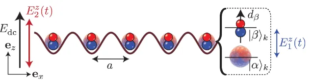
Figure 1. Schematic illustration of a system of polar molecules loaded into subsequent sites of a 1D optical lattice with site separation a. The molecules are aligned by a static electric field in theez-direction, Edc, and exposed to two
time-dependent microwave fields E1z(t)and E2z(t), both linearly polarized along thez-axis.
2. The system
We consider particles loaded into an optical lattice in a regime where the lattice is sufficiently deep so that tunnelling can be neglected on the timescale of the experiment. We assume that the particles have two internal states, one of which exhibits a strong dipole–dipole interaction, while the other is weakly interacting. This can be realized for realistic experimental parameters with either
1. Polar molecules in an external electric field, where a microwave coupling of rotational
states can give rise to dressed states with different dipole–dipole interactions, or
2. Neutral atoms in an external electric field coupled via a laser to excited Rydberg states,
which in contrast to the ground states exhibit a strong dipole–dipole interaction.
Below we summarize the key points of each of these implementations. Further details of polar molecules and neutral atoms coupled to excited Rydberg states are given in section 6.1 and section6.2, respectively.
2.1. Polar molecules
Polar molecules in their electronic-vibrational ground-state manifold possess a number of features that make them appealing to design and implement specific spin models. In addition to their electric structure, allowing e.g. for optical trapping, they have a rich internal (rotational) symmetry, with level spacings in the GHz regime, and negligible decoherence. They possess a permanent dipole moment d0 (typically of the order of a few Debyes [23, 24]) along the internuclear axis, which makes it possible to strongly couple their rotational excitations via static and microwave fields and gives rise to dipole–dipole interactions between different molecules.
We consider a 1D optical lattice (lattice spacing a) along the ex-axis with one polar
molecule trapped at each lattice site in the lowest vibrational state φk(x)(see figure1), which
implementation is that a suitable choice of E2z(t)makes it possible to cancel the induced dipole moment in one of the dressed states, and we denote the complete state of an atom in this dressed state at sitek as|αik. The single molecule ground state, which obtains a strong dipole moment
from the static electric field, is denoted as |βik. In the case when Edc and E
z
2(t)are properly
tuned, two molecules at distinct sites k and l that are in the states |βik and |βil lead to an
energy shift due to the dipole–dipole interaction potential ofVdd/|k−l|3. In section6.1, we give
example experimental parameters showing that an energy shiftVdd≈0.7d02/4π0a3≈10h¯ kHz
can be achieved. Note that we can therefore assume that the molecules remain in their motional ground state, since the band separation (trapping frequency)ωTis typically of the order of many
tens of kHz up to 100 kHz in a realistic scenario. Finally, the states |βik and|αik on all sites
k are coupled by a weak microwave field E1z(t)with Rabi frequencyand detuningδ, which gives rise to the effective microscopic many-body model that is described in section2.3below.
2.2. Neutral atoms coupled to Rydberg states
Neutral atoms in an external electric field exhibit strong dipole–dipole interactions when in certain Rydberg states with relatively large principal quantum number. For alkali atoms in states with principal quantum number n=17, it is possible to obtain a dipole moment of more than one kiloDebye (see section 6.2 for details). By finding isolated Rydberg states, the internal dynamics of each atom can be reduced to a two-level system, where weakly interacting atoms in the ground state are coupled via a laser to these states with large dipole–dipole interactions.
We assume that either atoms are loaded into a deep optical lattice with tight radial confinement, so that we have one atom per site along a 1D tube, or that we have weak radial confinement and many atoms per site (as occurs, e.g., when an optical lattice is applied along only one direction). In each case, we can assume that the ground-state atoms are confined to a single modefunction at each given lattice site, φk(x). In the case of a single atom per site, this
is the Wannier function for the lowest Bloch band, which is analogous to the case of the polar molecules described above. For many atoms per site, interactions can populate higher bands, and φk(x)will depend on the interactions. However, we assume that the timescale for excitation to
the Rydberg state is much shorter than timescales corresponding to the atomic motion and that therefore we can neglect population of any modefunction other than the initial modefunction φk(x) for either the ground or Rydberg states. We then assume that we can have at most one
excitation per lattice site, which in the case of large single-site populations is made possible by the Rydberg blockade mechanism, when we ensure that the blockade radius is larger than the occupied region at any single lattice site (see section6.2). This makes it possible to describe the system with an effective spin-1/2 model, assigning a state on each lattice site to the existence or non-existence of an atom in an excited Rydberg state on that site, labelled for site k by the states|βik and|αik, respectively.
In comparison with polar molecules, the dipole–dipole interaction of the strongly interacting state for Rydberg atoms is much larger. If we choose a principal quantum number
2.3. The effective model
In either the polar molecule or neutral atom case, we can derive the same effective microscopic model for the system in a frame rotating with the frequency of the field coupling the two internal states. We assume that at most one particle per site can be in the strongly interacting state, and represent the two possible states (weakly and strongly interacting) at each lattice site as two spin states. We label these states for site k as {|βik,|αik}, where |βik is the state exhibiting
strong dipole–dipole interactions, and|αik the non-interacting state. The Hamiltonian can then
be formulated as (h¯ ≡1)
ˆ
H =X
k
ˆ
σx k −δ
X
k
ˆ
nk+
Vdd
2
X
k6=m
ˆ nknˆm
|k−m|3, (1)
withnˆk ≡ |βihβ|k being the local ‘number operator’ for the interacting state at sitek. The Pauli
matrices are defined viaσˆx
k ≡ |βihα|k+|αihβ|k andσˆkz≡ |βihβ|k− |αihα|k, where the latter is
related to the number operators vianˆk=(σˆkz+ 1)/2.denotes the effective Rabi frequency and
δthe detuning of the laser, which excites the particles.Vddis the dipole–dipole interaction energy shift between neighbouring sites. Note that we assume the particles remain in the motional states φk(x)and also neglect corrections to the|k−m|−3 decay due to the finite width ofφk(x)(see
section6for more details).
Below we will first study the ground-state properties of this model, which will give us target states for the dynamical preparation process. We will then study the time dependence of this system starting from a many-body state where all of the particles are weakly interacting (Nk|αik), and investigate the adiabatic preparation of crystalline states as the parameters are
varied.
It is interesting to note that for an infinite system, the Hamiltonian can be written as
ˆ
HS=X
k
ˆ
σx k +
1
2(ζ(3)Vdd−δ)
X k ˆ σz k + Vdd 8 X
k6=m
ˆ
σz kσˆ
z m
|k−m|3 (2)
where we have removed constant terms, and ζ(3)≡P
kk−
3
≈1.202 denotes Apéry’s constant [27]. Note that in the case ofδ=ζ(3)Vdd, the system is equivalent to an Ising model in a transverse field with dipolar interactions. Ground states of this model have also been studied in [28].
3. Numerical method
To calculate the many-body dynamics and ground states of Hamiltonian (1), we make use of the TEBD algorithm as introduced in [21, 22]. This algorithm makes possible the near-exact integration of the Schrödinger equation for 1D lattice and spin Hamiltonians based on a matrix product state ansatz, and has been applied to a range of such Hamiltonians with nearest-neighbour interactions. There are also applications of matrix product state algorithms to dissipative systems [29]–[31], and these methods have been incorporated within density matrix renormalization group algorithms [32,33]. There is also a strong effort to extend these ideas to higher dimensions [34].
product state representation. This adds a computational cost ofO(l)basic operations compared to the standard TEBD calculation. Here we work with finite systems of size N, and always properly represent interactions over the full length of the system, i.e. l=N−1. This method of swapping also allows us to consider periodic boundary conditions for the dipole–dipole interactions. Note that we always perform convergence tests in the matrix product state bond-dimension χ and other numerical parameters4. For larger system sizes, swapping sites can become inefficient, in part due to the higher required values of χ. To implement interaction terms over substantially larger distances than in this study, more efficient algorithms should be used, e.g. algorithms involving the use of matrix product operators [36]–[38].
4. Ground states of the effective model
We begin by studying the key ground-state properties of the effective model of Hamiltonian (1). This will allow us to determine in which parameter regimes crystalline order will appear, and to characterize the states that will be the target states of the dynamical preparation process discussed next in section5.
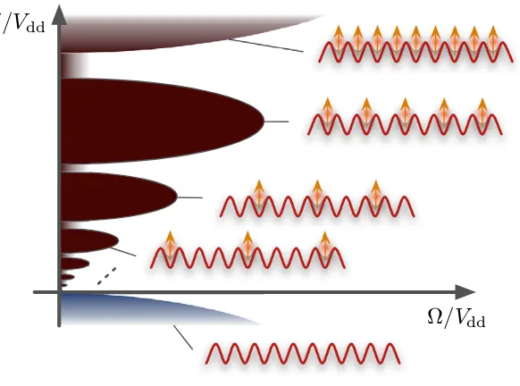
The Hamiltonian we study here has strong similarities to another model treated in several recent studies, in which the dipole–dipole interactions were replaced with van der Waals interactions arising for certain Rydberg systems [16]–[20]. In [17], it was shown that for=0 that system reduces to a classical spin model exhibiting a second-order phase transition from a paramagnetic to a crystalline phase at δ=0, and we observe similar behaviour here. Due to the dipolar long-range character we expect crystalline states with different periodicities of the excitations to the strongly interacting state to appear for δ >0 and small values of . The detuning plays the role of a chemical potential for strongly interacting states (or external magnetic field in the spin model), and it becomes favourable to excite states with a dipole–dipole interaction on the lattice. However, the long-range interactions will compete energetically with the detuning, leading to crystal periodicities that decrease with increasing δ/Vdd. Below we show that as the coupling /Vdd is increased, the crystalline order is broken, in favour of a paramagnetic phase in the spin language, with no long-range density–density ordering. These key features of the phase diagram are sketched in figure2.
We compute the ground state of equation (1) using the TEBD algorithm in several different parameter regimes. As a first step, we look at the total number of particles in a strongly interacting state|βi,
Nβ ≡
N
X
k
h ˆnki. (3)
In figure 3, we present a plot of Nβ for several detuningsδ and effective Rabi frequencies. We plot Nβ on a grid with spacings1δ=0.125Vdd and1=0.025Vdd.
As expected, for small/Vddthere is essentially no occupation of the strongly interacting states in regions with negative detuning, because a state with no|βik excitations is energetically
favoured. In contrast, a positive detuning leads to a reduction of the total energy when occupations of strongly interacting states are added to the system, and in regions with large positive detuning we find states with occupation of |βik on all lattice sites. In the region in
between, we observe varying excitation numbers depending on the choice of parameters. In
δ/Vdd
[image:12.595.158.449.120.336.2]Ω/Vdd
Figure 2. A sketch of the key features of the phase diagram for the system with Hamiltonian (1). For δ <0 and /Vdd1, the ground state involves all of the atoms in the non-interacting state in order to minimize the interaction energy (marked by the blue lobe). As the detuning δ >0 is increased, it becomes favourable to add excitations to the system, but this competes with an increasing interaction energy. This competition gives rise to crystalline phases with periodicities determined by this competition (marked by the brown lobes). For large /Vdd, the crystalline order is broken, but some particles exist in
excited states (white area).
[image:12.595.149.388.495.634.2]Figure 4.Fluctuation of the total occupation number of the strongly interacting state in a 50-site system with open boundary conditions as a function of for δ=1.1Vdd. The inset shows a zoom into the region 0.05Vdd660.5Vdd.
particular, there is a large plateau in the region 0.5Vdd.δ.2Vddand.0.1Vdd, in whichNβ
remains close to N/2=25. In the plot the contours of fillings slightly smaller (Nβ =23) and larger (Nβ=27) than N/2 are drawn as lines on theδ–plane. Note that the N/2 plateau lobe is centred around a value slightly larger thanδ=1, which is approximately the point where the second term in equation (2) vanishes and our system becomes an effective Ising spin model.
The half filling plateau disappears with increasing and we find a linear interpolation between regions with zero and full filling in this regime. This is consistent with a breakdown of the crystalline structure, and we note that in the limit→ ∞for finiteδwe expect the filling to be constant atN/2 since the stateNN
k (|βik− |αik)/
√
2 becomes the ground state of the system. Note that the grid is too coarse-grained to resolve plateaus of smaller fractions of the filling. However, we observe several kinks in the particle number at small values of/Vdd. We show below, e.g., that the feature at δ≈0.25Vdd corresponds to a crystalline state with filling N/3. This will verify the lobe-like structure as depicted in figure2; however, we find that the plateau for filling N/3 is significantly smaller, at values of≈10−2V
dd. For values ofδ∼2.25Vddwe
also observe some kinks, which correspond to regular patterns in the lattice with two subsequent sites being in the strongly interacting state, followed by one site being in the state|αik.
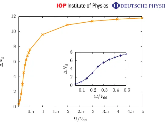
In order to illustrate the claim that the plateaus seem to belong to crystalline states, we can investigate the fluctuation in the total occupation number of the strongly interacting state,
1Nβ≡
N
X
k,l
h ˆnknˆli −Nβ2. (4)
In figure4, we show1Nβ forδ=1.1Vddand 0.05Vdd665Vdd. We find that1Nβdecreases significantly with decreasing and crossover behaviour is centred around ≈0.2Vdd. For .0.2 a crystalline state with nearly no fluctuations1Nβ.3N =50 is present. For large , 1Nβ converges to a value close to N/4=12.5, which is the correct result for finite δ and → ∞, i.e. whereNN
k (|βik− |αik)/
√
that the quantity 1Nβ is related to the Mandel Q-factor Q≡1Nβ/Nβ−1, which has been measured in recent experiments for the number of Rydberg excitations in small ensembles of cold atoms [39] and quantifies the deviation from a Poissonian number statistic [40].
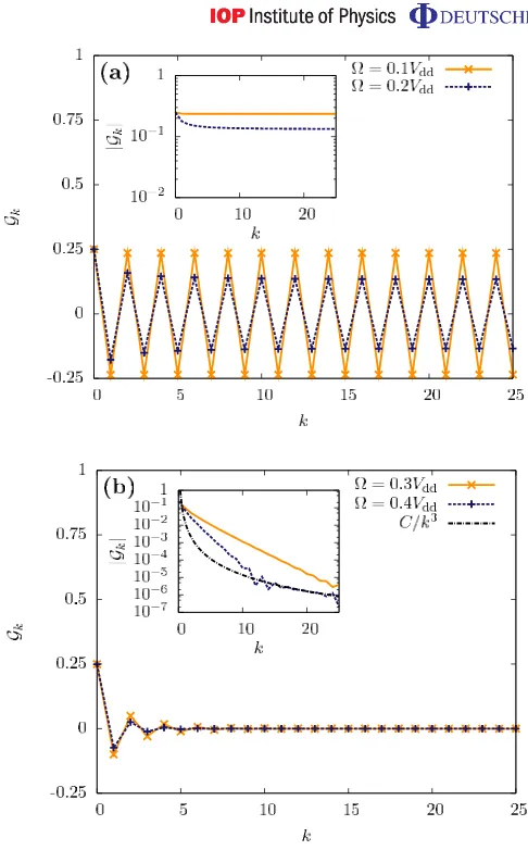
To study ground states in more detail for different parameter regimes and demonstrate clearly the crystalline behaviour, we evaluate DDC functions, defined as
Gk[i]≡ h ˆninˆi+ki − h ˆniih ˆni+ki. (5)
In a finite system with open boundary conditions, the exact values ofGk[i]will differ from sitei
where the DDC is evaluated. However, decay behaviour of the correlation functions for largek
should be independent of the site indexi in a sufficiently large system. To distinguish ground-state phases by their decay behaviour, we will first calculate ground ground-states of a system with periodic boundary conditions, in which the DDC becomes site independent. We then drop the site index and writeGk.
In figure5(a), we show a characteristic DDC in the parameter regime where the filling of the lattice is approximately N/2, choosing a detuning ofδ=1.1Vdd, with both=0.1Vddand =0.2Vdd. The inset in figure 5(a) shows the modulus of the correlation function,|Gk|, on a
logarithmic scale. In the regime of the half filling plateau we indeed find a crystalline structure with a pronounced zigzag pattern. The long-range crystalline order is indicated by the decay of
|Gk|to a non-zero value as a function of the site indexk. We find that for increasing N the value
of the constant to which|Gk|decays becomes independent of the system size.
We note, already from the comparison in figure5(a), that as /Vddincreases the strength
of the long-range crystalline order decreases. If we continue to increase /Vdd, we find that
this order is broken entirely, as shown in figure 5(b), with the same parameters, but for Rabi frequencies =0.3Vdd and =0.4Vdd. In these cases, we also observe peaks with periodicity 2; however, these occur only for very small values of k.5. As k increases, |Gk|
decays to zero, indicating the breakdown of the long-range order. This appears as a phase transition from crystalline order to essentially a ‘paramagnetic phase’, in which the correlations typically decay exponentially. However, we note here a special feature of the correlation functions in this parameter regime, specifically that while we have exponential decay at short distances (k.10), this changes to a power-law decay at longer distances. This is most clearly seen in the results for=0.4Vddin figure5(b). By fitting a function we find that, in this region, |Gk| ≈C/k3, with a constant C. This is the same power-law decay as the interaction term,
consistent with similar results derived for other long-range spin models [28, 41]. Physically, the correlations initially decay exponentially due to the primary influence on a given particle being from its nearest neighbours (analogous to exponentially decaying correlations in the paramagnetic phase of an Ising model). However, once correlations arising from nearest-neighbour interactions become sufficiently small, long-distance correlations will be dominated by the effects of the direct interaction between distant particles. Thus, long-range correlations are expected to decay at large distances with the same power as the interaction [41].
We find similar behaviour for crystalline states at other densities, including occupation periodicities larger than two. When the detuning is decreased from δ≈0.5Vdd it becomes less favourable to occupy |βik states in the system and therefore in the case of small ,
crystalline phases with larger spacing between these occupations appear in order to reduce the dipole–dipole interaction energy. For example, in figure 6 we show the DDC indicating an occupation of the states|βik on every third site for∼10−2Vddandδ=0.25Vdd. To make this
Figure 5. DDC functions Gk for the ground states of Hamiltonian (1) for
δ=1.1Vdd and (a) =0.1Vdd 0.2Vdd, and (b) =0.3Vdd, 0.4Vdd. The insets
show the modulus |Gk| on a logarithmic scale. Here we show the results for
a system with 50 sites and periodic boundary conditions. We find states with a marked crystalline structure of periodicity 2 in (a) and a phase transition at 0.2Vdd< <0.3Vdd in terms of the decay behaviour of|Gk|. In contrast to (a),
in (b)|Gk|decays exponentially. In the case of=0.4Vddthe long-range decay
behaviour (k&10) follows a power-law decay∝C k−3(withC≈1.7×10⁻²).
we observe the characteristic long-range order in the DDC, combined with a marked peak on every third lattice site. Again we find a phase transition away from crystalline order, with an exponential decay of |Gk|exhibited for larger values of. Note that the crystalline phase with
1/3 filling occurs in a much smaller region of parameter space than the crystalline phase with 1/2 filling.
Figure 6. DDC functions Gk for the ground states of Hamiltonian (1) for
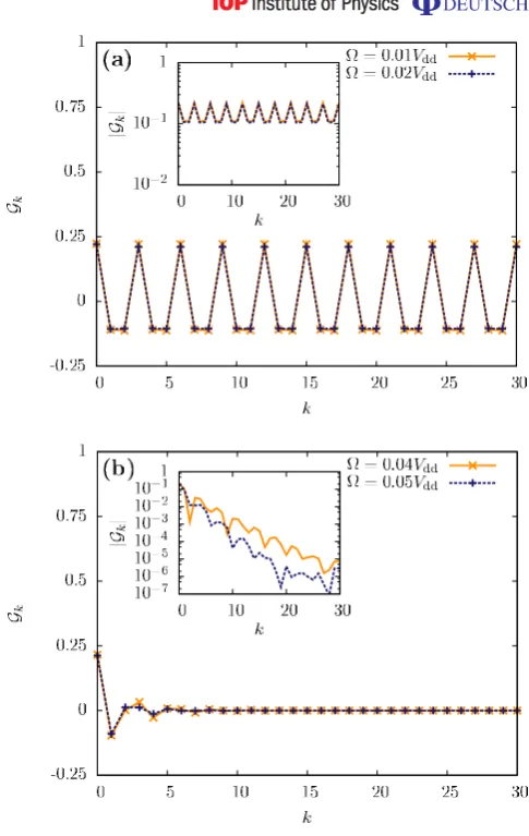
δ=0.25Vdd and (a) =0.01Vdd, 0.02Vdd and (b) =0.04Vdd, 0.05Vdd. The insets show the modulus |Gk| on a logarithmic scale. Here we show the results
for a system with 60 sites and periodic boundary conditions. We find a marked crystalline structure in (a) with periodicity 3 and a phase transition at around ≈0.03Vddindicated by the exponential decay behaviour of|Gk|in (b).
for an infinite system, we focus on the case of open boundary conditions relevant to the experiments. Although the correlation functions are modified by the boundary conditions, we show below that the characteristic signatures of different phases can still be clearly identified.
In figure 7, we show the DDC evaluated from site number 5 of an N =50 site system, i.e. Gk[5] with open boundary conditions. We choose the same parameters as were shown in figures 5(a) and (b), including crystalline phases with periodicity 2. Despite obvious effects of the open boundary conditions, we can clearly distinguish crystalline behaviour (=0.1Vdd,0.2Vdd) from the case where exponentially decaying DDCs are present (=
0.3Vdd,0.4Vdd). While in the crystalline phase we find very little decay for increasing k until
Figure 7.DDC functions evaluated from site indexi=5 in a 50-site system with open boundary conditions, Gk[5]. The results shown are for the same parameter regime as in figure5. Despite strong boundary effects, a crystalline phase is still distinguishable from a phase with such a structure via the behaviour over short rangesk.10. In the crystalline phase, the long-range decay follows a power-law behaviour proportional toC k−3(C ≈1.7×10⁻²is a constant).
rapidly decay below values of 10−5. As in figure 5 we still observe a long-range power-law
decay fork&10 proportional tok−3.
In relation to figure2, the results presented in figures5–7give evidence for the crystalline phases at filling factors 1/2 and 1/3 on the lattice, and show that for each there exist transitions as is increased to non-crystalline phases. This justifies that the lobes are finite along the -axis, and shows that the boundary depicted corresponds to a phase transition.
Note that the DDC functions can be measured experimentally both for Rydberg atoms and for polar molecules. Detection of these correlation functions is discussed in more detail in section6.
5. Dynamical creation of crystalline states
5.1. Time-dependent state preparation
We now discuss the dynamical creation of crystalline states in our system. The natural initial state for the experiments corresponds to having all of the particles in the non-interacting states
|αik, which would be the ground states for neutral atoms, or a single dressed rotational state
for polar molecules. In terms of the effective model, this state is the ground state of the Hamiltonian (1) for large negative detuning and small . The question now is whether one can time dependently vary the laser parametersandδ, i.e. find a trajectory in the–δ plane, so that this initial state is adiabatically transferred to a crystalline state of the form discussed in section4.
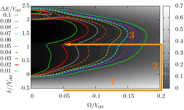
Figure 8. Shaded plot of the energy gap 1E between the ground and the first excited state as a function of and δ. The results are from exact calculations for an eight-site system with Hamiltonian (1). The lines indicate the contours of constant1E. A path, which consists of three segments and yields an adiabatic passage to a crystalline ground state, is sketched as an orange arrow (see text).
can then estimate possible paths for the adiabatic transfer based on the size of the energy gap 1E between the ground state and excited states. During the adiabatic ramp, we would like 1E to remain as large as possible to suppress non-adiabatic transitions to excited states of the effective model. In figure8, we show a shaded plot of the energy gap between the ground state and the first excited state as a function of and δ, with lines of constant energy gap marked in the plot. Close to=0, we find a large region where the energy gap assumes small values and where one can recognize lobe-like structures. Lobes at values ofδ≈2.25Vddare especially visible. As mentioned before, these correspond to states with regular patterns of two subsequent sites being in the strongly interacting state. In contrast to the lobe for filling fraction N/3 of the strongly interacting state at δ≈0.25Vdd, these are enhanced due to the larger increase
in interaction energy when adding single occupations of the strongly interacting state to the system. Therefore, these lobes are more robust when increasing . In general, the system is too small to observe lobes of filling fractions N/3 and smaller and these are only visible as small kinks for δ≈0.25Vdd. With increasing Rabi frequency the energy gap increases. The
requirement of having at any instance of time a sufficiently large energy gap is most easily fulfilled if one chooses to ‘steer’ a path in parameter space around those regions where the gap is the smallest. A simple path that seems to achieve this is, for example, to first increase at constant large negative detuning δ and then increase δ at a constant large . Both steps can be achieved by changing the parameters δ and rapidly, due to the large gap 1E present at all times. Afterwards, can be decreased to a small value on a line of constant δ. This path consisting of three segments is marked in figure8by an orange arrow.
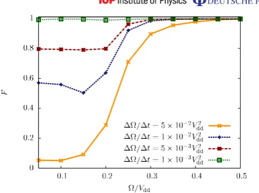
Figure 9.The fidelity of the adiabatically evolved state with the current ground state, when changing from 0.50Vdd to 0.05Vdd at constant δ=1.1Vdd in
segment 3 of the adiabatic preparation path. Results are shown for different variation rates 1/1t within a 30-site system with Hamiltonian (1). For decreasing variation rates the final fidelity for the crystalline state (at =
0.05Vdd) increases towards 1.
a crystalline state with excitation periodicity 2, which is the ground state of our model for the parameters=0.05Vddandδ=1.1Vdd. We perform real-time simulations for a path consisting of three segments, as sketched in figure8. We start at=0.05Vddand δ= −3Vdd. There, the inner product between the ground state of the Hamiltonian and the state in which all atoms are in the|αik state is sufficiently large for all system sizes. The segments of the path are
1. We increasefrom 0.05Vddto 0.5Vddatδ= −3 with a variation rate1/1t=0.05V2 dd.
2. We increaseδfrom−3Vddto 1.1Vddat=0.5Vddwith a variation rate1δ/1t =0.05Vdd2.
3. We decreasefrom 0.5Vddto 0.05Vddwith several variation rates1/1t.
Due to the large gaps in the energy spectrum it is possible for segments 1 and 2 to obtain states with a high fidelity F≡ |h9G(, δ)|9(t)i|2∼1 in the comparison of our evolved state,|9(t)i,
with the ground state of the effective model with the corresponding parameters |9G(, δ)i
on that path. The most sensitive part of this process is the third segment. In figure 9, we show the fidelity F of the adiabatically evolved state along segment 3 as a function of (t)
and for various variation rates 1/1t. On N =30 lattice sites, we find that for the three rates 1/1t=5×10−2V
dd,1×10−2Vdd and 5×10⁻³Vdd, this fidelity drops below values
of 80%, which occurs when crossing the phase transition from figure 5, i.e. in the regime 0.2Vdd< <0.3Vdd. At this point the ground-state gap becomes too small and excitations to higher excited states analogous to Landau–Zener tunnelling processes occur. However, when using a rate of 1/1t =1×10⁻³Vdd, we find that the fraction of the state that is lost into
higher excitations remains reasonably small and the final fidelity with the crystalline state at =0.05Vdd is larger than F ≈99%. Thus, we have shown that a crystalline state can be
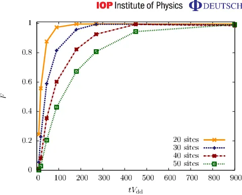
Figure 10.The fidelity of the time-evolved state with the target crystalline state, at =0.05Vdd, and δ=1.1Vdd as a function of time required for segment 3. Here we show results for several system sizes of 20, 30, 40 and 50 lattice sites. This fidelity decreases with increasing system size and with decreasing preparation time.
for all three segments is of the order of 500/Vdd, and we will show that this is experimentally
realizable for our two physical implementations below.
In an experiment with either polar molecules or neutral atoms coupled to excited Rydberg states in an optical lattice, the final state could be characterized by measuring DDC functions. These can be most easily detected directly by in situ imaging experiments [42]. In the case of polar molecules, the crystalline structure will be visible in noise-correlation measurements of state-selective momentum distributions of molecules released from the lattice [43]–[45]. In these correlation measurements, the periodicity of the crystalline structure would be present as a peak at the corresponding reciprocal lattice vector. In the case of Rydberg excitations, direct measurement of DDC functions could also be made by imaging the sample on a channel plate detector [20].
An important question is: To what extent can the same fidelities we have observed for a system size of 30 lattice sites also be achieved for larger system sizes? In general, we expect the energy gap between ground and excited states to become smaller with increasing system size, and we expect the measure of the fidelity to become more sensitive due to the exponentially increasing size of the Hilbert space. To analyse how much this affects the final fidelity, in figure10we plot the fidelity achieved after ramping the laser parameters through all segments of our preparation procedure, as a function of the time required for the final segment 3. We consider system sizes of 20, 30, 40 and 50 sites.
We find that for all system sizes the fidelity is>94% when choosing a variation rate slower than1/1t=1×10−3Vdd2, which corresponds to an operation time of approximately 450/Vdd
on segment 3. In the case of an even slower rate of1/1t=5×10−4Vdd2, which requires a time of approximately 900/Vdd, the fidelity becomes larger than 98%, even in the case of a system
5.2. Comparison with experimental parameters
Let us compare the time required to reach this final crystalline phase with experimentally accessible timescales, which are in general limited by the finite lifetime of the strongly interacting state. In the scheme presented above, at the slowest variation rate of 1/1t =
5×10⁻⁴V2
dd on segment 3, a total operation time of the order of 1000/Vdd is required. Note
that this time can be further dramatically decreased by choosing shorter paths or by not using a constant ramping rate but rather reducing it with time while approaching the critical point of the phase transition.
In the case of the polar molecule implementation (see section 6.1 for more details), typical parameters give Vdd≈10h¯ kHz, assuming a permanent dipole moment d0=1 Debye
and a lattice spacing of a=400 nm. This translates to a time for the complete preparation of approximately 0.1 s, which is significantly shorter than recently measured lifetimes of molecules in an optical lattice of 8 s [46]. By choosing polar molecules with larger dipole moments like LiCs (d0≈5.5 Debye [24]), the preparation time can be further reduced down to the order of a few ms.
In the case of the Rydberg atom implementation (see section 6.2 for more details), if we choose a principal quantum number n=14, then Vdd≈7h¯ GHz (assuming a lattice spacing of a=400 nm). Hence, the total operation time corresponds to approximately 140 ns in the experiment. This value is well below the typical lifetime of ann=14 Rydberg level of lithium, which can be found to be approximately 2.2µs [47]. Note that these estimates neglect the effects of blackbody radiation, which can redistribute the population among excited levels. For Rydberg atoms, in general the lifetime increases with increasing n and, furthermore, the required operation time decreases asn−4. However, the disadvantage of large principal quantum numbers is the small-level distances1interand1intra(see figure13), which both decrease withn.
This limits the experimentally accessible values of δ. In case n=14 (a=400 nm) at an electric field strength of Fel=100 kVm−1, we can estimate by using the results known from the hydrogen atom 1inter≈4.6×10³Vdd and1intra≈90Vdd. The field strength is thereby well
below the Inglis–Teller limit, which is in this case 319 kVm−1[48]. This justifies the validity of our two-level model, derived in section6.2, in this regime.
This comparison to the lifetime of a single Rydberg atom is oversimplified, as in the presence ofNβexcited atoms, the rate of single decay events will increase roughly in proportion to Nβ.5However, as the system size (and henceNβ) becomes larger, the effect of a single decay on the crystalline structure should decrease. While the many-body state fidelity will be very sensitive to a single decay, DDC functions should be robust, at least on length scales smaller than those separating places where spontaneous emissions have occurred. The effect on the many-body state of single decay events also depends on when during the excitation process they occur. A full treatment of this excitation process including decay events could be achieved by studying the dynamics of a master equation including spontaneous emission events.
Therefore and from the results in figure10, we conclude that the adiabatic passage should be experimentally realizable for both our implementations of the effective spin model with a size of∼50 sites. For larger system sizes, longer timescales will be required for reaching fidelities as high as those we have obtained here. However, the properties of the final states will typically be determined in an experiment by the measurement of correlation functions. In contrast to the
5 This neglects superradiant effects, which should be small as the excitations are separated by distances of the
state fidelity, correlation functions (together with the physical character of the state) become more robust to small non-adiabaticities (especially those resulting in localized defects) in larger systems.
6. Physical implementations of a long-range spin model
6.1. Polar molecules in an optical lattice
In the following, we describe how to implement Hamiltonian (1) with a system of polar molecules. We consider N molecules confined to the lowest motional level on subsequent sites of a deep 1D optical lattice, with modefunction φk(x) on site k. We assume that the
lattice is sufficiently deep so that tunnelling between wells of the lattice is strongly suppressed on typical experimental timescales. In particular, we consider molecules in their electronic vibrational ground-state manifold with a closed shell structure 16, which possess permanent
dipole moments (e.g.40K87Rb-like in recent experiments [7]). The setup is depicted in figure1.
We use a strong and a weak microwave field linearly polarized along thez-axis and an additional static field aligned along the same direction. Given the fact that we consider samples of the order of a few to 100µm, one can neglect the spatial variation of the respective static and microwave fields along the optical lattice axis, which is aligned in theex-direction.
The low-energy spectrum of a single molecule at site k in our setup is well described by rotational excitations, governed by a rigid rotor Hamiltonian coupled to the fields via an electric dipole interaction [50]–[53]
ˆ
Hrotk (t)=BJˆ2k− ˆdkz Edc+E1z(t)+E2z(t). (6)
Here, B is the rotational constant typically of the order of tens of GHz (h¯ ≡1) [26], Jˆk
is the angular momentum operator, dˆkz is the z-component of the dipole operator and Edc,
E1z(t)= E1zexp(−iω1t)+ c.c.and E2z(t)= E
z
2exp(−iω2t)+ c.c.are the static, weak and strong
external microwave fields, respectively. The eigenstates of Jˆ2
k are denoted by |J,mJik with eigenvalues J(J+ 1) (¯h≡1),
and mJ = −J, . . . ,J being the eigenvalues of the projection onto the z-axis, Jˆ z k. The
dipole operator dˆkz couples rotational states with differences 1J = ±1, and we recall that the eigenstates of equation (6) have no net dipole moment. The non-vanishing elements of the operator dˆkz are given by hJ±1,mJ| ˆd
z
k|J,mJik=d0(J,mJ;1,0|J±1,
mJ)(J,0;1,0|J±1,0)
√
(2J+ 1)/(2(J±1)+ 1)in terms of the Clebsch–Gordan coefficients (J1,m1;J2,m2|J,m), where d0 denotes the permanent electric dipole moment along the
internuclear axis, which is typically of the order of a few Debyes [23,24].
By applying electric fields, one lifts the degeneracy of the state manifolds with J >0 and induces a finite dipole moment in the dressed rotational states. Since the fields are aligned along the quantization axis,mJ is conserved, and we focus on states withmJ =0 in our setup, which
are connected to the ground state. The induced dipole moments of two molecules at distinct siteskandl then lead to an energy shift due to the dipole–dipole interaction potential.
is valid provided that the band separation ωT is substantially larger than the laser coupling
parameters and interaction energies. Thus, we can expand the field operators as
ˆ
9σ(x)= X
k
φk(x)gˆkσ (7)
and identify individual molecules occupying each mode described by the operators gˆkσ. Since all rotational states we consider here have mJ =0, they are only coupled by an interaction
proportional to dˆkzdˆlz, which can be integrated over the modefunctions in each lattice site. The resulting many-body Hamiltonian of a system for N molecules can be written as
ˆ
Hpm(t)≈
N
X
k
ˆ
Hrotk (t)+Vdd(1)
N
X
k6=l
ˆ dkzdˆlz
|k−l|3, (8)
with lattice spacing a, and where Vdd(1)≈1/(8π0a3). Note that we neglected corrections to
the shape of the interactions, which are of the order ofO(lH/(a|k−l|)), wherelH denotes the characteristic harmonic oscillator length for the optical potential well on each site.
A suitable choice of external electric fields then makes it possible to strongly couple/dress locally two (effective) rotational levels, such that only one level has a strong induced dipole moment, while at the same time the transition dipole moment remains negligibly small. This results in dipole–dipole interactions in equation (8) reducing to the diagonal form of equation (1).
We now detail our appropriate choice of electric fields for obtaining the desired dressed states. The key idea is to apply the static field Edc for inducing a finite dipole moment in the
rotational states, leading to the dressed states |Jidc, defined by [BJˆ2k− ˆd z
kEdc]|Jidc=EJ|Jidc
(see figure11(b)), and to then couple the two states|1idc and|2idcby a strong microwave field E2z(t), such that the dipole moment vanishes in one of the resulting dressed states. The field
E2z(t)is tuned to the transition between the two states with Rabi frequency2≡ h2| ˆdkz|1idcE2z
and detuning12≡ω2−(E2−E1)(see figure11). Diagonalizing the corresponding two-level
Hamiltonian and making the rotating wave approximation lead to the two dressed states
|α±ik =cos(θ/2)|1idc−sin(θ/2)|2idc with the dressing angleθ ≡arctan(−22/12)(0< θ <
2π), where the state|α−ik (|α+ik) corresponds toθ < π (θ > π). The corresponding energies of
the dressed states are E±
α =E1−12/2± p
12
2+ 422/2.
Finally, we couple the state |αik≡ |α−ik and the state |βik ≡ |0idc by the weak electric
field with Rabi frequency 1≡ hα| ˆdkz|βikE z
1 and detuning 11≡ω1−(Eα−E0). Thereby we
assume that the field E1z(t) is much weaker than E2z(t), so that the states |αi and |βi are unaffected by E1z(t). Going to the rotating frame and making the rotating wave approximation the many-body Hamiltonian becomes time independent and reads
ˆ
Hpm=1
N
X
k
ˆ
σx k −11
N
X
k
ˆ
nk+V(
1) dd
N
X
k6=l
ˆ
Vd
|k−l|3, (9)
with σˆx ≡ |βihα|k+|αihβ|k and nˆk≡ |βihβ|k. In the last term of equation (9), Vˆd is the
Figure 11. Level scheme for a system of polar molecules in a combination of static and microwave fields, cf figure 1. (a) Energy levels EJ of a molecule
in a static electric field Edc. The field orients the dipoles, i.e. induces finite permanent dipole moments in each rotational state|Jidc. (b) A strong linearly polarized microwave field E2z(t)couples the states|1idc and|2idc with the Rabi
frequency2and detuning12. Fine-tuning the microwave field (with respect to
the static field) makes it possible to cancel the permanent dipole moment in one of two dressed states, |α+iand |α−i, cfdα→0. A second (weaker) microwave
field E1z(t)finally couples the ground state |βi ≡ |0idc to the dressed state with
vanishing dipole|αiwith an effective Rabi frequency1and detuning11.
{|αik|αil,|αik|βil,|βik|αil,|βik|βil}is
ˆ
Vd≡
dα2 0 0 0
0 dαdβ dβα2 0
0 d2
βα dαdβ 0
0 0 0 dβ2
(10)
Here,dα≡ hα| ˆdkz|αik,dβ≡ hβ| ˆdkz|βik anddβα ≡ hβ| ˆdzk|αikare the dressed single-particle dipole
operator elements.
Our goal is to find values of the microwave dressing angleθ and of the static field strength
Edc, for which the permanent dipole moment dα and the transition dipole momentdβα become negligible compared to the permanent dipole moment dβ. Then the only remaining entry in equation (10) is dβ2, such that a dipole–dipole interaction is only present if both molecules are in the strongly interacting state|βik.
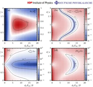
To this purpose, we compute the respective values of dα, dβα and dβ as a function of the microwave field angle θ and the electric field strengths up to Edc=25d0/B. Figure 12
summarizes our results. In particular, in figure 12(a) (figure 12(b)) we show the ratio of the permanent dipole moments in the two states,dα/dβ (the ratio of the transition dipole moments
dβα/dβ), as a function of Edc=25d0/B andθ. The solid lines show contours of constant ratio.
Figure 12. Effective dipole moments of a molecule in a combination of static and microwave fields, Edc and E2z(t). (a) The dipole moment dβ (in units of d0) induced by the static electric field. (b) The ratio dα/dβ of the two permanent dipole moments and (c) the ratiodβα/dβof the transition to permanent dipole moment as a function of the static-field strength d0Edc/B and the
microwave-dressing angleθ. (d) The relative deviation,δVdd/dβ2, of the induced
dipole–dipole coupling with respect to the model interaction (1) as a function of
d0Edc/B andθ. The thick solid lines show the contours of (b) vanishing dipole
moment dα and (c) vanishing transition dipole moment dαβ. The white circle indicates the point for which one has vanishing deviations, i.e. one obtains an exact implementation of the effective model.
solid lines). We note that the two respective contour lines intersect at a specific parameter pair (E◦
dc≈15.65B/d0, θ◦≈0.93π)(white circle). For these parameters one obtains an exact
implementation of model (1).
To quantify a deviation from an exact implementation of Hamiltonian (1) for general parameters (Edc, θ)6=(Edc◦, θ◦), in figure 12(c) we plot the (normalized) deviation from the model,δVd/dβ2, given by
δVd ≡ k ˆVd−dβ2|βik|βilhβ|khβ|lk =
q
d4
α+ 2dβα4 + 2dα2dβ2. (11)
Since the transition dipole moment enters only quadratically into the last expression, we note that the error around the optimal point closely resembles the contour line of vanishing
fine-tuning the microwave field allows us to obtain deviations δVd.10−2d2
β, while the
permanent dipole moment dβ≈0.8d0. Thus, to a good approximation, we obtain the model interaction with a typical timescale of Vdd≡2dβ2Vdd(1)≈dβ2/4π0a3≈10¯hkHz for typical
parameters (a=400 nm,dβ=0.8 Debye).
6.2. Neutral atoms coupled to Rydberg states
In this section, we show how to implement spin Hamiltonian (1) by making use of neutral atoms coupled to excited Rydberg states. We consider alkali atoms confined in an optical lattice in a single tube, with inter-site distanceaoriented along thex-direction. Perpendicular to the lattice a homogeneous electric field,F=Felez, is applied, together with a laser that couples the ground
state|giof each atom to a specific chosen Rydberg–Stark state.
6.2.1. Dipole–dipole interaction. While the atomic ground state is only slightly shifted
by the external electric field, the level structure of high-lying Rydberg states is strongly altered compared to the field-free case. Nevertheless, the azimuthal symmetry of the atomic Hamiltonian is preserved such thatm(the quantum number of thez-component of the electronic orbital angular momentumLz) remains a good quantum number [48]. States with large quantum
defect, i.e. usually s- and p-states, sustain a second-order Stark shift, while the degenerate states with higher angular momentum exhibit a linear Stark effect, reminiscent of the hydrogen atom [54]. The derivative of the energy with respect to the electric field strength directly yields the electric dipole moment of the given state. While the precise level structure, and therefore the dipole moment of the Stark states, depends on the element under consideration, the exact results known from the hydrogen atom usually provide good estimates for the quantities of interest.
A sketch of a Rydberg–Stark level structure is shown in figure 13. For sufficiently small field strengths, i.e. below the Inglis–Teller limit where the atom becomes ionized, the levels are grouped in manifolds, which can be labelled by the principal quantum number n. In this study, we focus on the energetically highest state of such a manifold whose azimuthal quantum number ism=0. Employing the formula for hydrogen, the electric dipole moment of this state, which we denote as|dni, evaluates to
dn=dnez=32ea0n(n−1)ez, (12)
witheanda0being the charge of the electron and the Bohr radius, respectively.
Two atoms excited to the states |dnik and |dnil at distinct sites of the lattices k andl are
expected to interact strongly via the dipole–dipole interaction potential, as already for n=17 equation (12) gives a dipole moment of more than 1 kiloDebye. We intend to work in a regime in which the interaction can be treated within first-order perturbation carried out in single-particle product states. To this end it is important to note that the dipole–dipole interaction commutes with Lz1+Lz2 and therefore only couples atomic pair states for which the azimuthal quantum
numbers obey m1+m2=m0
1+m02 [8]. We assume that all these couplings are far off-resonant,
which can be ensured by properly tuning 1intra and 1inter using the electric field. Moreover,
accidental resonances can be avoided by restricting oneself to low principal quantum numbers
E
Fel
n n+ 1
|g
|dn
∆intra
∆inter
δ
[image:27.595.152.458.94.291.2]Ω0
Figure 13.Sketch of the level structure of an alkali metal atom as a function of the electric field strength. The energy of hydrogen-like states grows linearly with the field strengthFel. Low angular momentum states with quantum defect exhibit a second-order Stark effect. In our scheme, we couple the ground state|giof an atom to the Rydberg state |dni, which exhibits the strongest Stark shift within
the givenn-manifold. The magnetic field strength and the laser parameters are set such that1intra.1inter,1intra |δ|and1intra0.
excitations unlikely. Employingdn⊥ex, the interaction Hamiltonian between two atoms being
in the product state|dnik|dnil can then be written as
ˆ
Hklint=2Vdd(1) d
2
n
|k−l|3|dnik|dnilhdn|khdn|l, (13)
with Vdd(1)≈1/(8π0a3), when the confinement length in each lattice site is much smaller than
the lattice spacing.
We now turn to the description of the interaction between the laser and the atom. We employ a two-level approximation assuming that the ground state |gik is coupled only to
the state |dnik. This is justified as long as the modulus of the laser detuning δ and the Rabi
frequency0are much smaller than the energy gaps1intraand1inter. Making the rotating wave
approximation, the interaction of the laser with an atom located on thekth site can be written as (h¯ =1)
ˆ
HLk =0(|dnikhg|k+|gikhdn|k)−δ|dnikhdn|k (14)
with0andδbeing the Rabi frequency and the detuning, respectively.
6.2.2. Many-body model. We now consider the many-body physics when many atoms in an
optical lattice are simultaneously coupled to the state |dnik. We assume that either atoms are
![Figure 7. DDC functions evaluated from site index i = 5 in a 50-site system withopen boundary conditions, G[5]k](https://thumb-us.123doks.com/thumbv2/123dok_us/1696235.123012/17.595.146.389.94.302/figure-ddc-functions-evaluated-index-withopen-boundary-conditions.webp)