This is a repository copy of Experimental study of heat transfer in oscillatory gas flow inside a parallel-plate channel with imposed axial temperature gradient.
White Rose Research Online URL for this paper: http://eprints.whiterose.ac.uk/79565/
Version: Accepted Version
Article:
Yu, Z, Mao, X and Jaworski, AJ (2014) Experimental study of heat transfer in oscillatory gas flow inside a parallel-plate channel with imposed axial temperature gradient.
International Journal of Heat and Mass Transfer, 77. 1023 - 1032. ISSN 0017-9310 https://doi.org/10.1016/j.ijheatmasstransfer.2014.06.031
[email protected] https://eprints.whiterose.ac.uk/
Reuse
Unless indicated otherwise, fulltext items are protected by copyright with all rights reserved. The copyright exception in section 29 of the Copyright, Designs and Patents Act 1988 allows the making of a single copy solely for the purpose of non-commercial research or private study within the limits of fair dealing. The publisher or other rights-holder may allow further reproduction and re-use of this version - refer to the White Rose Research Online record for this item. Where records identify the publisher as the copyright holder, users can verify any specific terms of use on the publisher’s website.
Takedown
If you consider content in White Rose Research Online to be in breach of UK law, please notify us by
Heat transfer in an oscillatory gas flow inside a parallel-plate channel with
imposed axial temperature gradient
Zhibin Yu, Xiaoan Mao and Artur J. Jaworski1
Department of Engineering, University of Leicester University Road, Leicester LE1 7RH, UK
1
Corresponding author: [email protected]; T: +44(0)113 343 4871
Abstract
Understanding of heat transfer processes between a solid boundary and an oscillatory gas flow is
important for the design of internal components such as heat exchangers, regenerators and thermal
buffer tubes in thermoacoustic and Stirling thermodynamic machines where the flow oscillations
are part of the power production or transfer processes. The heat transfer between the flow and an
arrangement of hot and cold plates forming a parallel-plate channel is studied experimentally and
numerically. Here, the particular focus is on the processes occurring within the thermal and viscous
boundary layers. The measured phase-dependent temperature fields combined with the velocity
fields are studied in detail. Near wall temperature minima and maxima of the cross sectional
temperature profiles are observed when the gas moves from cold to hot or from hot to cold parts of
the channel. They are referred to as "temperature undershoot" and "overshoot", respectively. The
existence of these temperature minima and maxima causes large local temperature gradients in the
direction normal to the wall, which result in large heat diffusion between gas layers in the direction
normal to the wall. It is observed that the flow history has a strong impact on the temperature fields.
This invalidates the so-called "Iguchi hypothesis", based on which the heat transfer data for steady
flows is being applied to oscillatory flow conditions. General guidelines for the design of heat
exchangers used in thermoacoustic devices are discussed.
1. Introduction
Heat transfer processes in the presence of oscillatory flows have received a lot of research interest
in the past few decades. The heat transfer enhanced due to the oscillatory flow may lead to a large
variety of possible applications. Therefore a large number of experimental and numerical works
have been carried out, and some examples are given in Refs. [1-8]. On the other hand, a variety of
devices such as Stirling engines or coolers, thermoacoustic devices and pulse tube coolers employ
the oscillatory gas flow of the working fluid as a means of energy transfer. Therefore, the design of
heat exchangers, stacks/regenerators and thermal buffer tubes in such devices requires the
understanding of the heat transfer process between the solid boundary and oscillatory gas flow.
General reviews of the heat transfer processes in the presence of oscillatory flow have been given
by Cooper et al. [9], Zhao and Cheng [10], and Sert and Beskok [11]. Kurzweg and Zhao [12] and
Kurzweg [13, 14] have been first to develop a concept of the so-called “dream pipe”, which used
the sinusoidal oscillation of water flow to enhance the heat transfer in a pipe between the cold and
hot reservoirs. The mechanism of this enhancement was attributed to: (i) the phase lag occurring
between the fluid in the centre and that near the wall; and (ii) transverse heat transfer between these
two parts of fluid, and the enhanced axial heat transfer due to the oscillatory displacement of the
fluid along the pipe [12-13].
Subsequently, Zhao and Kurzweg [15] also conducted numerical simulations of their dream pipe.
Neglecting the motion of the fluid within the penetration depth in the near wall region, they treated
this part of fluid as a thermal capacity for heat accumulation. The penetration depth due to thermal
diffusion is defined as 2 , with being the thermal diffusivity and the angular frequency of
the oscillation. Ozawa and Kawamoto [16] pointed out that such a treatment did not account for the
time-dependent temperature profiles near the channel wall. They developed a lumped-parameter
heat transfer model to simulate the dream pipe with water as working fluid at a frequency of less
than 1 Hz. The simulations agreed with the time-dependent temperature fields in the dream pipe
qualitatively (the temperature being measured using a thermo-sensitive liquid–crystal tracer
technique). Their research showed that the isotherms change significantly from the shape of upward peak to that with a downward peak. The change of the isotherm’s shape followed that of the velocity profile with a certain phase lag. In addition to Zhao and Kurzweg’s understanding of the
mechanism of heat transfer enhancement mentioned above, Ozawa and Kawamoto [16] revealed
of the fluid motion between the fluid in the channel centre and near the wall also played an
important role in such heat transfer enhancement.
Zhao and Cheng [17] investigated a laminar oscillatory flow in a heated pipe numerically. An “annular effect” in the temperature profiles near the entrance of the pipe was observed. This is characterised by a temperature minimum or maximum near the wall rather than at the centre of the
flow channel, when the wall is at a temperature higher or lower than the bulk flow. This annular
effect in the temperature profiles becomes more pronounced with the increase of the kinetic
Reynolds number, Re = D2/, where D is the channel width and is the fluid kinematic viscosity.
The presence of the annular effect was also verified by the numerical simulation of an oscillatory
flow in a channel carried out by Sert and Beskok [11]. In their model, the middle portion of the top
plate was uniformly heated and its two sides were kept at a constant temperature, while the bottom
plate was insulated. It was reported that for an oscillatory flow with a Womersley number ( =
2
D ) of 10, large cross-sectional temperature variations were observed in the temperature
fields, which are much less significant in the temperature fields when the Womersley number is at 1
when the annular effect in the velocity profiles is not present. It was understood that these
temperature distributions in the channel were highly affected by the velocity profile. It is
immediately clear to see that the Womersley number is the square root of the kinetic Reynolds
number, Re . The forced convection due to the flow motion increases with the increase of the
penetration depth, Womersley number and Prandtl number (ratio of momentum and thermal
diffusivities). Furthermore, they reported that the corresponding steady unidirectional forced
convection was even more effective than the oscillatory flow forced convection for the tested case.
It seems that the abovementioned “annular effects” represent the same kind of phenomena as the
so-called upward and downward peaks in isotherms observed by Ozawa and Kawamoto [16].
Liao et al. [2] applied a channelled oscillatory air flow to cool microprocessor chips. They reported
that there are two different heat transfer enhancement mechanisms. When the Reynolds number, Re
= UmD/ defined on the maximum velocity of the imposed oscillatory flow, is small, the heat
transfer enhancement is mainly due to the reduction of Stokes' layer thickness, 2 , with the
increase of the oscillation frequency. While in the high Reynolds number region, the heat transfer is
enhanced due to the presence of the higher-order harmonics of imposed flow frequency. Li and
Yang [18] investigated numerically the heat transfer in reciprocating flows at low frequencies and
large amplitudes in short channels. They demonstrated a heat transfer enhancement due to the
separation. The intra-cycle oscillations were characterised by the axial velocity oscillations within
individual cycles, especially during the accelerating stage.
As can be seen, substantial progress has been made in understanding the mechanisms behind the
enhanced heat transfer in oscillatory flow. However it is also clear that such understanding is still
incomplete, in particular in terms of a simultaneous analysis of the time-resolved temperature and
velocity fields. Notably, previous research has been conducted to measure the overall heat transfer
coefficients in heat exchangers subjected to oscillatory flow for different specific applications [7,
19-22] and thus it did not consider the microscopic fluid flow and heat transfer behaviour. Very few
experimental research studies [16, 23-25] focused on the time-resolved temperature fields in
oscillatory conditions for some particular applications, however these did not attempt to combine
the temperature and velocity field (or fluid displacement) information.
It is also worth noting that most of the experimental studies mentioned above have been conducted
with incompressible fluids, such as liquid water, which has Prandtl number greater than 1. This
makes the viscous boundary layer thicker than the thermal boundary. As discussed above, the heat
transfer enhancement in oscillatory flow is mainly due to the interactions between the thermal and
viscous boundary layers. It remains unclear of how the effect of the Prandtl number on the heat
transfer processes is different in the cases when gases are used as the flow medium. Therefore, it
would be interesting to explore such interactions for a compressible medium (e.g. gas) in order to
mimic the actual situation encountered in thermoacoustic devices, Stirling engines and pulse tube
coolers.
The main objective of this work is to examine the time-dependent velocity and temperature fields
obtained experimentally in order to gain a better understanding of heat transfer processes in
thermoacoustic heat exchangers. In their previous work [26, 27] the authors demonstrated the use of
Planar Laser Induced Fluorescence (PLIF) and Particle Image Velocimetry (PIV) techniques to
measure time-dependent temperature and velocity fields, respectively, within a heat exchanger in a
thermoacoustic system. Here, these techniques are applied to acquire the velocity and temperature
fields in a parallel-plate channel in an oscillatory gas flow of one oscillation amplitude at a single
frequency. Due to the limitation of the current experimental setup, numerical simulation has been
developed to extend this examination to cover a range of oscillation amplitudes and operating
frequencies.
Furthermore, on the engineering design level, this research aims to provide further guidance to aid
hypothesis (i.e. each instant of the time-dependent flow depends only on that instant's velocity, not
on the flow history), is to use the data obtained for steady flows for the design of heat exchangers
for oscillatory flows [28, 29]. The Iguchi hypothesis is confirmed to be applicable at some
conditions when the oscillation amplitude is relatively large [30, 31]. However, as the displacement
of the gas is comparable with the length of the heat exchanger, one might question the validity of
this hypothesis. In this paper, this issue is also discussed on the basis of the obtained experimental
results. Furthermore, the principles of the heat exchanger design for thermoacoustic systems will
also be discussed.
2. Experimental method
The detailed description of the test rig and the experimental and measurement procedures can be
found in the already mentioned previous work [26, 27] and therefore only a brief description will be
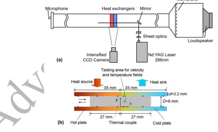
provided here. Figure 1a is a schematic illustration of the experimental apparatus. It is essentially a
7.4 m long quarter-wavelength resonator where the intensity of the acoustic excitation (and thus
fluid displacement amplitude) is controlled by the level of excitation provided by a loudspeaker
(sub-woofer). The resonator has a rectangular cross-section with internal dimensions 134 mm by
134 mm. The operating frequency of the test rig is 13.1 Hz.
Figure 1 (a) Schematic illustration of the experimental apparatus with PLIF system deployed (similar
setup for PIV is omitted); (b) close up of the test channel formed by a pair of “hot” and “cold” plates
[image:6.595.39.475.438.703.2]A pair of parallel-plate heat exchangers is placed inside the resonator, 4.6 m from the end plate
shown in Figure 1a, where the acoustic anti-node exists [27]. The “hot” heat exchanger is
constructed from a series of brass plates, each containing an embedded cable heater, used to control the plate temperature. The “cold” heat exchanger is constructed from a series of plates containing a meandering channel for cooling water. Both hot and cold plates have a length (l) of 35 mm along
the axial direction of the resonator, a width (w) of 132 mm in the transverse direction, and a
thickness (d) of 3.2 mm. The plates form a series of channels with a height (D) of 6 mm, and one of
them is schematically depicted in Fig. 1b. As a result, the Womersley number for the flow in these
channels is between 9.2 and 13.4, and the kinematic Reynolds number is in the range of 85–180,
due to the temperature dependent kinematic viscosity.
Twelve fine-wire K-type thermocouples (marked as dots in Fig. 1b) are placed on the surface of hot
and cold plates forming the test channel. There are three pairs on cold plates. They are 3.0, 17.5 and
32.0 mm away from the joint (i.e. x = 0), respectively. Symmetrically to the joint, there are also
three pairs on the hot plates as shown in Fig. 1b. The thermocouples monitor the temperature
distribution on the hot and cold plates. A PID temperature controller (Omega Model CN8592) is
used to accurately control the temperature at the reference point (x = –32mm, y = 6 mm) to within
±1 ºC at a pre-set value of 200 ºC for the experiments in this paper. The cold plates are cooled to
around 30 ºC.
The arrangement described above allows obtaining oscillatory gas flow within the test channel,
maintained by the acoustic excitation. The measurement methodologies adopted in this work
include two-dimensional temperature and velocity field measurements using Planar Laser Induced
Fluorescence (PLIF) and Particle Image Velocimetry (PIV), respectively. By these means, the
temperature and velocity fields within the channels can be obtained and thus the heat transfer
between the oscillatory gas flow and the cold and hot plates can be studied.
Generally, the rationale behind the current experimental arrangement is to use the hot and cold
plates to mimic the fins of respective heat exchangers that are often part of heat engines which
employ oscillatory gas flow, e.g. thermoacoustic engines, pulsed tube coolers or Stirling engines. In
the channels shown in Fig.1b, the hydraulic radius, rh, defined as ratio of the gas volume to the wet
area, is 3 mm. It is of the same order of the thermal penetration depth ( = 2/ ) and viscous
penetration depths ( = 2 / ). These two characteristic lengths are often used with oscillatory
of 1/ [32]. They are used as approximate criteria for determining the fin spacing [29]. The thermal
penetration depth, k, is in the range of 0.7–1.2 mm, and the viscous penetration depth in the
range of 0.6–mm along the channel, when the temperature dependent thermal diffusivity and
kinematic viscosity of air are considered.
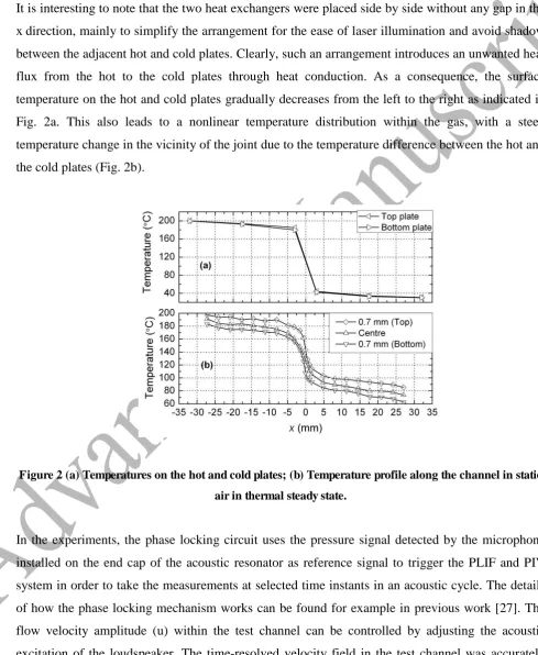
It is interesting to note that the two heat exchangers were placed side by side without any gap in the
x direction, mainly to simplify the arrangement for the ease of laser illumination and avoid shadow
between the adjacent hot and cold plates. Clearly, such an arrangement introduces an unwanted heat
flux from the hot to the cold plates through heat conduction. As a consequence, the surface
temperature on the hot and cold plates gradually decreases from the left to the right as indicated in
Fig. 2a. This also leads to a nonlinear temperature distribution within the gas, with a steep
temperature change in the vicinity of the joint due to the temperature difference between the hot and
the cold plates (Fig. 2b).
Figure 2 (a) Temperatures on the hot and cold plates; (b) Temperature profile along the channel in static
air in thermal steady state.
In the experiments, the phase locking circuit uses the pressure signal detected by the microphone
installed on the end cap of the acoustic resonator as reference signal to trigger the PLIF and PIV
system in order to take the measurements at selected time instants in an acoustic cycle. The details
of how the phase locking mechanism works can be found for example in previous work [27]. The
flow velocity amplitude (u) within the test channel can be controlled by adjusting the acoustic
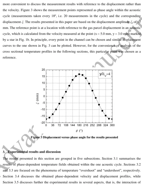
[image:8.595.42.532.164.761.2]measured by PIV. The measured velocity, u, can be converted to the gas parcel displacement, ,
using = u/ , with the velocity leading the displacement by 90º in phase. In this paper, it is often
more convenient to discuss the measurement results with reference to the displacement rather than
the velocity. Figure 3 shows the measurement points represented as phase angle within the acoustic
cycle (measurements taken every 18º, i.e. 20 measurements in the cycle) and the corresponding
displacement . The results presented in this paper are based on the displacement amplitude a of 17
mm. The reference point is at a location with reference to the gas parcel displacement in an acoustic
cycle, which is calculated from the velocity measured at the point (x = 5.0 mm, y = 3.0 mm) marked
by a star in Fig. 1b. In principle, every point in the channel can be chosen and similar displacement
curves to the one shown in Fig. 3 can be plotted. However, for the convenience of analysis of the
cross sectional temperature profiles in the following sections, this particular point was chosen as a
[image:9.595.47.543.91.737.2]reference.
Figure 3 Displacement versus phase angle for the results presented
3. Experimental results and discussion
The results presented in this section are grouped in five subsections. Section 3.1 summarises the
results of phase-dependent temperature fields obtained within the one acoustic cycle. Sections 3.2
and 3.3 are focused on the phenomena of temperature “overshoot” and “undershoot”, respectively.
Section 3.4 discusses the obtained phase-dependent velocity and displacement profiles, while
Section 3.5 discusses further the experimental results in several aspects, that is, the interaction of
velocity and temperature fields, the effect of the "flow history" on the oscillatory flow behaviour
Section 4 containing the results from a numerical study of the same arrangement in a number of
flow oscillation amplitudes and frequencies.
3.1Temperature fields in one acoustic cycle
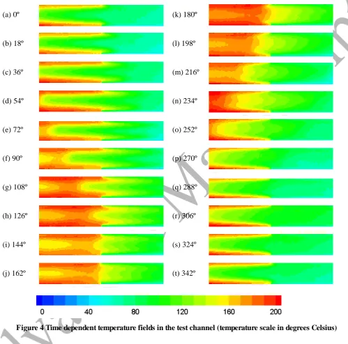
Figure 4 shows the two-dimensional temperature field distribution in the cross-section parallel to
the flow direction for 20 phases obtained for the displacement amplitude a of 17 mm. At phase=
0º, the fluid displacement reaches the negative maximum value, which means that the gas parcel in
the channel moves farthest to the left (as can be inferred from Fig. 3). It can be seen that, at this
instant, the cold gas moves into the hot channel. However, this penetration is only pronounced in
the central area of the channel. Adjacent to each hot plate, there is a thin layer of gas with high
temperature, which seems not to be affected by the cold gas coming from the cold channel.
After this phase, the gas parcel starts to accelerate to move to the right. From phase = 0º to = 90º
the gas moves from the displacement farthest left into the equilibrium location as shown in Fig. 3.
From the temperature image, it can be found that the cold gas gradually flows out from the hot
channel after being partially heated. The hot gas, which was heated and has been pushed out from
the hot channel at the end of the previous acoustic cycle, gradually takes over the left end of the hot
channel. From phase = 18º to = 90º, it can be observed that two layers of gas with relatively
high temperature (as shown in orange) gradually penetrate into the cold channel. It can be found
that these two layers of gas have higher temperatures than those of the gas either in the centre of the
channel or adjacent to the cold plates. As a result, a temperature maximum is present in this layer,
rather than at the centre of the channel or on the wall. This feature of the temperature field is
referred to as "temperature overshoot".
At phase = 90º, the gas reaches the equilibrium position, and the velocity reaches the maximum.
After this time instant, the gas starts to move to the right while beginning to decelerate. It can be
seen that the central area at the right of the hot channel still shows relatively low temperatures at
this phase. This indicates that during the preceding quarter of the acoustic cycle ( = 0–90º), the
heat transfer from the hot plate to the gas has not influenced the gas temperature in the central area
significantly. The “temperature overshoot” effect seems very strong at phase = 90º and becomes
even more pronounced at = 108º and = 126º. Subsequently, the effect weakens and practically
disappears at phase = 180º. From Fig. 4, it can be seen that most of the cold channel is still
substantially when it was previously present in the hot channel during phases between = 0 and
90º.
(a) 0º (k) 180º
(b) 18º (l) 198º
(c) 36º (m) 216º
(d) 54º (n) 234º
(e) 72º (o) 252º
(f) 90º (p) 270º
(g) 108º (q) 288º
(h) 126º (r) 306º
(i) 144º (s) 324º
[image:11.595.53.553.126.620.2](j) 162º (t) 342º
Figure 4 Time dependent temperature fields in the test channel (temperature scale in degrees Celsius)
At phase = 180º, the gas reaches farthest to the right in the channel. After this instant, the gas
starts to move to the left, reaching the equilibrium position by phase = 270º. The gas transfers
heat to the cold plates during this period. By inspecting the temperature fields (c.f. the right end of
342º, the gas accelerates to move to the left end of the channel. After it reaches the farthest left end
( = 360º or = 0º), it enters the next acoustic cycle.
It should also be noted that, the temperature fields are slightly asymmetric relative to the centreline
of the channel. This is mainly due to the accumulated residual heat in the void space in the
resonator to the left of the hot plates. This is caused by the natural buoyancy effect over time, often
an hour or so that is necessary for the calibration and measurement using PLIF technique. This
asymmetry can also be seen from the gas temperature profiles along the channel in Fig.2 – the gas
near the top plate is slightly hotter than that close to the bottom plate.
3.2Temperature profiles of "temperature overshoot"
As shown in Section 3.1, the “temperature overshoot” effect only exists in the cold channel when
the gas flows to the right. It will be interesting to investigate further the phase-dependent
cross-sectional temperature profiles within the cold channel within this type of flow. Following the
normalisation proposed by Zhao and Cheng [10], the normalised fluid temperature is expressed as
C H w f T T T T (1)
where , Tf, Tw, TH and TC are normalised fluid temperature, local fluid temperature, wall
temperature, reference hot temperature (here 200 ºC), reference cold temperature (here 30 ºC),
respectively. The distance from the bottom plate, y is normalised using the viscous penetration
depth, . An average viscous penetration depth (i.e. a= 0.75 mm) is used as the characteristic
length.
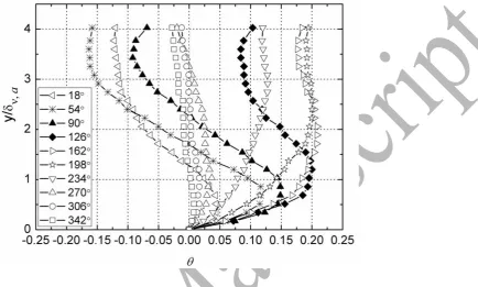
Fig. 5 shows the normalised temperature profiles for ten selected phases at a location 5.0 mm away
from the joint into the cold channel (x = 5.0 mm). For simplicity, only the temperature profiles at
the bottom half of the channel are presented. At = 0–90º, the temperature profiles have peaks with
y/a less than 1, while the gas moves from the left to its equilibrium position with increasing speed.
The peak temperature is substantially higher than the gas temperature in the channel centre. With
the gas moving further right, the temperature peak moves away to the centre and reaches y/a = 2
when = 162º. Further on, the temperature peak continue to shift to the centre, and the peak
temperature starts to decrease ( = 198º and 234º); the gas temperature in the channel centre
in between the wall and the centre, but the "temperature overshoot" described above is much less
recognisable when the gas moves from the right to the left ( = 198–342º).
Figure 5 Cross-sectional temperature profiles for ten selected phases (x=5.0 mm). The temperature
[image:13.595.145.580.117.378.2]maxima near the wall for phases = 90º and = 126º (in solid symbols) can be seen.
Fig. 4 also shows that the temperature overshoot effect is very apparent near the joint between “cold” and “hot” channel, while it seems weaker further to right of the cold channel. However, it is difficult to judge from Fig. 4 whether there is a dependence of the temperature overshoot effect on
the location. Therefore, for the purpose of further analysis, the temperature profiles at different
locations, for a selected phase = 90º have been extracted and plotted as Fig. 6. Five locations have
been selected along the cold channel from left to the right with x changing from 5 mm to 25 mm
with a step of 5 mm. It can be found from Fig. 6 that the shape of the individual temperature
profiles is quite similar, while the location of the temperature peak moves slightly below y/a = 1
to slightly above. The magnitude of the temperature overshoot effect seems to differ from location
to location. However, from Fig.2, one can hypothesize that this dependency is mostly likely due to
the nonlinear temperature profile along the channel. One can see that the temperature gradient
dTm/dx decreases when x increases from 5 mm to 25 mm. This will be discussed further in Section
Figure 6 Cross sectional temperature profiles for different locations along the cold channel ( = 90º).
The temperature peaks shown in Fig. 5 indicate that the gas temperature at the peak point is
considerably higher than those near the centre and plate surface. Therefore, it would be interesting
to find out the actual temperature differences from the data before normalisation. Figure 7 shows
the extracted temperature differences between the maximum temperature of each profile Tmax and
the temperature in the centre of the channel Tcentre. For convenience of comparisons, it is also
plotted against location given in the legend of Fig. 6. It can be found that, the temperature
[image:14.595.29.545.156.715.2]difference is around 41 ºC for x = 5.0 mm and it decreases to around 13 ºC for x = 25.0 mm.
Figure 7 Difference between the maximum temperature and the temperature in the channel centre for
[image:14.595.29.479.455.713.2]3.3Temperature profiles of “temperature undershoot”
As already mentioned in Section 3.1 the effect of “temperature undershoot” exists in the hot channel
when the gas flows to the left. In an analogous way as that described in Section 3.2, the
phase-dependent temperature profiles of the cross sectional temperature fields in the hot channel can be
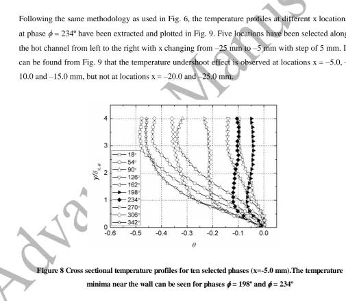
extracted. Fig. 8 shows such normalised phase temperature profiles at location x=–5.0 mm. The
temperature profiles exhibit an apparent minimum for y/a ~ 1 for phases of = 198º and = 234º.
However, these local temperature minima are not as pronounced as temperature maxima shown in
Fig. 5. For phase = 234º, the difference between the gas temperature at the channel centre and the
temperature minimum is only around 10 ºC.
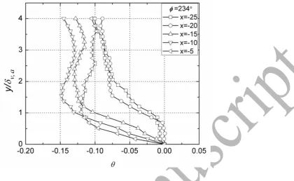
Following the same methodology as used in Fig. 6, the temperature profiles at different x locations
at phase = 234ºhave been extracted and plotted in Fig. 9. Five locations have been selected along
the hot channel from left to the right with x changing from –25 mm to –5 mm with step of 5 mm. It
can be found from Fig. 9 that the temperature undershoot effect is observed at locations x = –5.0, –
[image:15.595.29.535.267.706.2]10.0 and –15.0 mm, but not at locations x = –20.0 and –25.0 mm.
Figure 8 Cross sectional temperature profiles for ten selected phases (x=-5.0 mm).The temperature
Figure 9 Cross sectional temperature profiles for different locations along the hot channel ( = 234º)
3.4Phase-dependent velocity and displacement profiles
The experimental results discussed so far suggest that the instantaneous displacement of the gas parcels belonging to different “layers” of fluid (i.e. of different y distances away from the solid wall) is important for understanding the heat transfer processes between the fluid and the plate. As
described in Section 2, the velocity field measurements were performed for 20 phases in an acoustic
cycle. Fig. 10 shows the cross sectional velocity profiles for x = 5.0 mm, for all investigated 20
phases. Of course the amplitude of velocity depends on y. It increases from 0 to the maximum as y
increases from 0 to around 2.5aand then slightly decreases as y approaches the centre of the
channel. These “overshoots” of velocity are also known as “annular” effects and have been well
documented in the literature related to oscillatory flow, e.g. [17].
Similarly, when looking at profiles for individual phases in the cycle, one can see that the velocity
of gas parcels also depends on y. However it can also be seen that for two different values of y (i.e. for different fluid “layers”) the instantaneous values of velocities can have a relative phase lag – for example for phase = 0º and parcel at y = a it is positive, while in the channel centre it is
negative; and an opposite is true for phase = 180º. Furthermore, as the temperatures at two sides
of the selected x location (here x = 5 mm) are different, the gas experiences different viscous drag
temperature and this can cause asymmetries in the positive and negative displacement values. For these reasons the “bundle” of the phase-dependent velocity profiles appears as a slightly asymmetric pattern in Fig. 10.
Figure 10 Phase-dependent velocity profiles as function of y (x=5.0 mm)
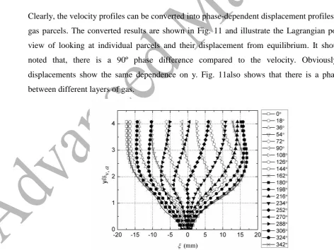
Clearly, the velocity profiles can be converted into phase-dependent displacement profiles of the
gas parcels. The converted results are shown in Fig. 11 and illustrate the Lagrangian point of
view of looking at individual parcels and their displacement from equilibrium. It should be
noted that, there is a 90º phase difference compared to the velocity. Obviously, the
displacements show the same dependence on y. Fig. 11also shows that there is a phase lag
between different layers of gas.
[image:17.595.35.508.375.729.2]3.5Discussion
Some of the important aspects of the discussion of the presented experimental results are the issues of the interactions between the velocity and temperature fields; the related influence of “flow history” on the flow behaviour; and the effects of over-/undershoots on the heat transfer. These are considered in the following subsections.
3.5.1 Interaction of velocity and temperature fields
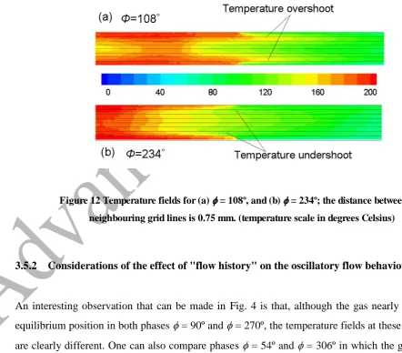
To better understand the underlying thermo-fluid mechanisms behind the temperature
overshoot/undershoot effects, it is helpful to compare selected temperature fields with the results
shown in Figs. 5 and 11. To this end, Fig. 12 illustrates “magnified” temperature fields obtained for
phases = 108º (Fig. 12a) and = 234º (Fig. 12b). Gridlines, with the relative distance between
them of a = 0.75 mm have been added to the temperature fields to help the discussion.
Looking at Fig. 12a, one can identify a thin layer of warm gas (denoted by orange colour, located
approximately between y = ,a and y = 2 ,a) which penetrates into the cold channel. However, it
can also be seen that the layer of gas adjacent to the surface of the cold plate (y < ,a) remains
relatively cold (as illustrated by green colour). Similarly, looking at Fig. 12b, it can be seen that a
thin layer of cold gas (denoted by green colour, located approximately between y = ,a and y =
2 ,apenetrates into the hot channel. However, it can also be seen that the layer of gas adjacent to
the surface of the hot plate (y < a) remains hot (as illustrated by red colour).
Looking at Fig. 11, one can find that the displacement of gas within the layer where y < ,a is in the
range of 5–6 mm taking the middle of the layer as reference. This means that most of fluid in this
layer has not travelled to the hot (cold) channel during the previous phases. Therefore, it is cooled
(heated) by the cold (hot) plate all the time. On the other hand, the gas in centre of the channel (say
y > 3 ,a) is not affected by the viscous drag effects from the wall. It moves with a higher
displacement amplitude. This part of gas is also not affected by the thermal diffusion from the wall.
Therefore, it practically keeps the temperature obtained from the static conditions. However, the gas
located between y = ,a and y = 3 ,a exhibits a much more complicated behaviour. For this part of
gas, the amplitude of displacement and changes in temperature both strongly depend on y. A
qualitative analysis of Figs. 11 and 12 suggests that this layer of gas moves with relatively high
displacement, but is also affected by the thermal diffusion from the wall. Therefore, the fluid can be
partially heated up when it is present in the hot channel (from = 0º to = 180º), and can be cooled
down during its presence in the cold channel (from = 180º to = 360º). From the Lagrangian
to the hot channel (i.e. the temperature overshoot shown in Fig. 12a), and local temperature
minimum (i.e. the temperature undershoot shown in Fig. 12b) can occur when the gas moves from
the cold to the hot channel. In addition, when looking at the displacement as a function of phase
angle for the fluid where y > 3 ,a and y < 3 ,a one can see that there is a relative phase difference
for the fluid near the centre and closer to the wall.
The current observations strongly suggest the temperature overshoot and undershoot effects
documented in this paper are essentially similar phenomena to those of “upward (downward) peaks
of isotherms” observed by Ozawa and Kawamoto [16] and the temperature “annular effects”
observed by Zhao and Cheng [17]. The results shown in Figs. 6 and 7 also suggest that the steeper
the temperature gradient, the stronger the temperature overshoot/undershoot effects become.
Furthermore, if there is no temperature gradient, temperature undershoot/overshoot effects will not
[image:19.595.40.483.359.747.2]occur. This is similar to findings of Zhao and Cheng [17], namely that there is not temperature “annular effect” in the middle of their heated pipe when no temperature gradient exists.
Figure 12 Temperature fields for (a) = 108º, and (b) = 234º; the distance between two
neighbouring grid lines is 0.75 mm. (temperature scale in degrees Celsius)
3.5.2 Considerations of the effect of "flow history" on the oscillatory flow behaviour
An interesting observation that can be made in Fig. 4 is that, although the gas nearly reaches the
equilibrium position in both phases = 90º and = 270º, the temperature fields at these two phases
are clearly different. One can also compare phases = 54º and = 306º in which the gas parcel is
54ºbut not at phase = 306º. Other pairs of such images can also be compared. This illustrates
simply the fact that the flow history (i.e. temperature distribution within the fluid in all preceding
phases) determines the pattern of temperature distribution at the phase of interest.
However, despite the unique and complicated characteristics of oscillatory flows, the engineering
design of the heat exchangers for oscillatory situations uses results and data from research in steady
flows, because there are few relevant experimental and numerical studies made in oscillatory flows,
and those available are not being widely used due to their fragmentary character.
One of the typical approaches is to use the steady flow correlations available to determine the heat
transfer coefficient in order to estimate the time averaged temperature difference between the
oscillating gas and solid surface, using RMS value of Reynolds number as an input for the
calculations [29]. Such treatment is based on the so-called Iguchi hypothesis, i.e. that each instant of
the time-dependent flow depends only on that instant’s velocity, not on the flow history. However,
the experimental results such as these presented here show that the Iguchi hypothesis is invalid for
heat transfer process in the oscillatory flow and therefore the current design procedures and
calculations are strictly not suitable.
3.5.3 Effects of temperature overshoot/undershoot on the heat transfer
According to Fig. 6, the difference between the temperature peak and the temperature of gas in the
channel centre or at the wall is in the order of tens of degrees Celsius. These temperature
differentials clearly exist within the transverse distances in the order of ,a. Therefore, the
transverse temperature gradients caused by these temperature differences are in the order of 10,000
ºC/m, which is very high. They lead to the transverse heat exchange processes between gas layers
and this is the mechanism behind enhancing the transverse heat transfer between the plate surface
and the gas. Furthermore, the inhomogeneous temperature profiles also enhance the axial heat
transfer along the channel. This type of heat transfer enhancement is beneficial for heat exchangers
subjected to oscillatory flow.
In thermal buffer tubes of thermoacoustic engines, and pulse tubes of pulse tube coolers, a large
temperature difference is produced by ways such as mechanical power input and is required to be
maintained by virtue of stratified flow and ideally linear temperature distribution [29]. Such
increase the heat transfer along the temperature gradient and will inevitably lead to heat (or cooling)
losses.
On the other hand, the results obtained in this work show on the microscopic level of individual
flow channels that the gas outside y > 2.5 is practically not affected by the thermal diffusion from
the channel wall. The heat exchangers to be used in oscillatory flow often require a greater heat
transfer area for a given overall size. Hence, advised by this analysis, the distance between the solid
heat transfer surfaces, such as fins, could be around 4–5 times to keep the heat transfer surfaces
closely packed, while not at a cost of much greater pressure drop due to the viscous losses.
4. Numerical simulation and results
The oscillatory flow produced in the current experimental apparatus is limited to a single frequency
and one oscillation amplitude. To overcome this shortcoming, the computational tool was
introduced to extend the examination discussed above to a range of frequencies and oscillation
amplitudes. The details of the numerical scheme are available in [33]. The complete set of
continuity, momentum and energy equations is solved over a computational domain that covers the
pair of heat exchangers and a length of 270 mm either way from the joint of hot and cold plates.
The same geometrical configuration as that used in the experiments is adopted. The boundary
conditions for the inlet and outlet of the domain are pre-defined [31], with the resonator wall set as
adiabatic. The temperature distribution on the surface of the heat exchanger plates is introduced into
the computational model. The modelled operating conditions are listed in Table 1, all at
atmospheric pressure. The simulation was validated by comparing the flow fields against the
experimental results and a good agreement was reached (omitted here for brevity). According to the
investigation in [31], laminar model is recommended when the displacement amplitude is small,
such as 17 mm, and the two-equation SST k– turbulence model should be used when the
displacement amplitude is higher.
Table 1 Operating conditions used in the numerical simulation
Cases Frequency (Hz)
Displacement amplitude (mm)
Womersley number,
Kinematic Reynolds number, Re
1 13.1 17 9.2 - 13.4 85 - 180
2 13.1 35 9.2 - 13.4 85 - 180
3 13.1 50 9.2 - 13.4 85 - 180
4 25 8.9 12.7- 18.6 162 - 345
The temperature profiles at x = 5.0 mm for ten selected phases are given in Fig. 13, when the
displacement amplitude is 17 mm, 35 mm and 50 mm respectively. The temperature profiles for a
= 17 mm is in general in agreement with the experimental results. The “temperature overshoot” is
clearly visible, in particular for = 54–126º. The effect of heat diffusion reaches beyond 3 ,a
which is quite different from the experimental observation. The actual reason remains unclear. The
gas temperature at the centre of the channel is higher in the numerical results, compared with the
measurements, especially at = 342º and 18º. This could be caused by the settings of the thermal
boundary conditions in the simulation, where the excessive heat can only leave the computational
domain through the inlet and outlet.
While the gas is subject to different excitation levels, the oscillatory flow shares the same
Womersley number due to the same frequency. Hence the Stokes’ boundary layer thickness is also
the same. However, it can be seen in Fig. 13 that the temperature peaks appear close to the cold
plate, when the displacement amplitude, thus the velocity amplitude, is bigger. Nevertheless, the
temperature overshoot effect is still clearly visible. The temperature peak moving closer to the solid
wall is understood to be caused by the change of the viscous boundary layer. Similar observation is
made in the hot channel.
Figure 13 Cross-sectional temperature profiles for ten selected phases (x=5.0 mm) at different oscillation
amplitudes (f = 13.1Hz)
Under the investigated frequencies (13.1–50 Hz), the velocity amplitude in the flow channel is kept
constant. Hence, the displacement amplitude decreases when the operating frequency increases. The
Womersley number of the oscillatory flow covers a range of 9.2–26.3. The temperature profiles at x
= 5.0 mm for ten selected phases are given in Fig. 14, when the operating frequency changes to 25
Hz and 50 Hz. The temperature overshoot effect is still clearly present. The temperature peaks are
located around 2 ,a from the solid wall and the magnitude of the temperature overshoot reduces
These are considered to be controlled by the displacement that the gas can travel within a cycle. For
a smaller displacement, the temperature change that gas can experience will be smaller, even if the
[image:23.595.160.585.123.258.2]temperature gradient is maintained the same.
Figure 14 Cross-sectional temperature profiles for ten selected phases (x=5.0 mm) at different operating
frequencies
5. Conclusion
This paper investigates the interaction between thermal and viscous boundary layers in a channel
with a nonlinear temperature gradient. The mechanism of the heat transfer associated with the
oscillatory flow has been analysed in detail. The phase lag between different layers of gas adjacent
to the wall leads to large transverse temperature gradient normal to the plate surface, which gives
rise to the temperature undershoot and overshoot phenomena in this research. These time dependent
transverse temperature gradients enhance the heat transfer between the gas and plates, as well as the
heat transfer along the channel. Furthermore, the experimental results indicate that the flow history
at the preceding phases would significantly affect the temperature distribution at subsequent phases.
This indicates the Iguchi hypothesis, which enables the application of the heat transfer data for
steady flows to the oscillatory flow conditions, may not always be reliable, at least at the conditions
studied in this work.
Acknowledgments
Artur J. Jaworski would like to acknowledge the support for his research programme in
fundamentals of thermoacoustics received from EPSRC under grants GR/S26842/01GR/T04502/01,
GR/T04519/01, EP/E044379/1 and EP/E044379/2 and thus for creating research training
opportunities for Drs Mao and Yu. Dr Lei Shi is acknowledged for his expert PIV and PLIF
measurements under the supervision of Dr Mao and data processing required to produce illustrative
References
1. Kaviany M and Reckker M, Performance of a heat exchanger based on enhanced heat diffusion
in fluids by oscillation: experiment, Journal of Heat Transfer, 112 (1) (1990) 56-63.
2. Liao QD, Yang KT and Nee VW, Enhanced microprocessor chip cooling by channelled
zero-mean oscillatory air flow, in: Hsu TR et al (Ed.), Proceedings of the International Intersociety
Electronic Packaging Conference, Advances in Electronic Packaging, EEP-Vol.10-2, ASME,
NY, 1995, pp. 789–794.
3. Beskok A and Warburton TC, Arbitrary Lagrangian Eulerian analysis of a bidirectional
micro-pump using spectral elements, International Journal Computational Engineering Science, 2(1)
(2001) 43–57.
4. Oddy MH, Santiago JG and Mikkelsen JC, Electrokinetic instability micromixing, Analytical
Chemistry, 73(24) (2001) 5822–5832.
5. Sert C and Beskok A, Oscillatory flow forced convection in micro heat spreaders, Numerical
Heat Transfer, Part A. 42(7) (2002) 685–705.
6. Paek I, Braun JE and Mongeau L, Characterizing heat transfer coefficients for heat exchangers
in standing wave thermoacoustic coolers, Journal of the Acoustical Society of America, 118 (4)
(2005) 2271-2280.
7. Nsofor EC, Celik S and Wang X, Experimental study on the heat transfer at the heat exchanger
of the thermoacoustic refrigerating system, Applied Thermal Engineering, 27 (14-15) (2007)
2435-2442.
8. Wakeland RS and Keolian RM ,Calculated effects of pressure-driven temperature oscillations
on heat exchangers in thermoacoustic devices with and without a stack, Journal of the
Acoustical Society of America, 116 (1)(2004) 294-302.
9. Cooper WL, Nee VW and Yang KT, Fluid mechanics of oscillatory and modulated flows and
associated applications in heat and mass transfer – a review, Journal of Energy, Heat and Mass
Transfer,15 (1993)1-19
10.Zhao TS and ChengP, Heat transfer in oscillatory flows, Annual Review of Heat Transfer, Tien
C-L (Ed.), IX (Chapter 7) (1998)
11.Sert C and Beskok A, Numerical simulation of reciprocating flow forced convection in
two-dimensional channels, Journal of Heat Transfer, 125 (2003)403-412.
12.Kurzweg UH and Zhao LD, Heat transfer by high-frequency oscillations: a new hydrodynamic
technique for achieving large effective thermal conductivities, Physics of Fluids, 27 (11) (1984)
13.KurzwegUH, Temporal and spatial distribution of heat flux in oscillating flow subjected to an
axial temperature gradient, International Journal of Heat and Mass Transfer, 29 (12) (1986)
1969-1977.
14.Kurzweg UH, Enhanced heat conduction in fluids subjected to sinusoidal oscillations, Journal of
Heat Transfer, 107 (2) (1985) 459-462.
15.Zhao AX and Kurzweg UH, Extension of the SIMPLE algorithm to heat transfer in
time-periodic flows with moving boundaries, Numerical Heat Transfer, Part B, 18 (1990) 189-203.
16.Ozawa M and Kawamoto A, Lumped-parameter modelling of heat transfer enhanced by
sinusoidal motion of fluid, International Journal of Heat and Mass Transfer, 34 (12) (1991)
3083-3095.
17.Zhao TS and Cheng P,A numerical solution to laminar forced convection in a heated pipe
subjected to a reciprocating flow, International Journal of Heat and Mass Transfer, 38 (16)
(1995) 3011-3022.
18.Li P and Yang KT, Mechanisms for the heat transfer enhancement in zero-mean oscillatory
flows in short channels, International Journal of Heat and MassTransfer,43 (2000) 3551–3566.
19.Mozurkewich G, Heat transfer from a cylinder in an acoustic standing wave, Journal of the
Acoustical Society of America, 98(4) (1995)2209-2216.
20.Leong KC and Jin LW, An experimental study of heat transfer in oscillating flow through a
channel filled with an aluminium foam, International Journal of Heat and Mass Transfer, 48
(2005)243–253.
21.Leong KC and Jin LW, Heat transfer of oscillating flow and steady flows in a channel filled
with porous media, International Communication of Heat and Mass Transfer, 31 (2004) 63–72.
22.Ozawa M, Shinoki M, Nagoshi K and Serizawa E, Scaling of heat transfer characteristics in an
oscillating flow, Journal of Enhanced Heat Transfer, 10(3) (2003)275-285.
23.Wetzel M and Herman C, Experimental study of thermoacoustic effects on a single plate part II:
heat transfer, Heat and Mass Transfer, 35 (6) (1999) 433-441.
24.Wetzel M and Herman C, Experimental study of thermoacoustic effects on a single plate part I:
temperature fields, Heat and Mass Transfer, 36 (1) (2000) 7-20.
25.Peattie RA and Budwig R, Heat transfer in laminar, oscillatory flow in cylindrical and conical
tubes, International Journal of Heat and Mass Transfer, 32 (5) (1989) 923-934.
26.Shi L, Mao X and Jaworski AJ, Application of planar laser induced fluorescence measurement
techniques to study heat transfer characteristics of parallel-plate heat exchangers in
27.Mao X and Jaworski AJ, Application of particle image velocimetry measurement techniques to
study turbulence characteristics of oscillatory flows around parallel-plate structures in
thermoacoustic devices, Measurement Science and Technology,21(3) (2010) 035403 (16pp).
28.Swift GW, Thermoacoustic engines, Journal of the Acoustical Society of America, 84 (1988)
1145-1180.
29.Swift GW, Thermoacoustics: A unifying perspective for some engines and refrigerators,
Acoustical Society of America, New York (2002).
30.Iguchi M, Ohmi M and Maegawa K, Analysis of free oscillating flow in a U-shaped tube,
Bulletin of the JSME, 25(207) (1982), 1398-1405.
31.Petculescu A and Wilen LA, Oscillatory flow in jet pumps: Nonlinear effects and minor losses,
Journal of the Acoustical Society of America, 113(3) (2003), 1282-1292.
32.Rott N, Damped and thermally driven acoustic oscillations in wide and narrow tubes, Zeitschrift
für Angewandte Mathematik und Physik, 29 (1969) 230–243.
33.MohdSaat FAZ and Jaworski AJ, Oscillatory flow and heat transfer within parallel-plate heat
exchangers of thermoacoustic systems, Proceedings of the World Congress on Engineering