Distributed energy efficient clouds over core networks

Distributed Energy Efficient Clouds Over

Core Networks

Ahmed Q. Lawey, Taisir E. H. El-Gorashi, and Jaafar M. H. Elmirghani

Abstract—In this paper, we introduce a framework for

design-ing energy efficient cloud computdesign-ing services over non-bypass IP/WDM core networks. We investigate network related factors including the centralization versus distribution of clouds and the impact of demand, content popularity and access frequency on the clouds placement, and cloud capability factors including the number of servers, switches and routers and amount of storage required in each cloud. We study the optimization of three cloud services: cloud content delivery, storage as a service (StaaS), and virtual machines (VMS) placement for processing applications. First, we develop a mixed integer linear programming (MILP) model to optimize cloud content delivery services. Our results indi-cate that replicating content into multiple clouds based on content popularity yields 43% total saving in power consumption com-pared to power un-aware centralized content delivery. Based on the model insights, we develop an energy efficient cloud content delivery heuristic, DEER-CD, with comparable power efficiency to the MILP results. Second, we extend the content delivery model to optimize StaaS applications. The results show that migrating content according to its access frequency yields up to 48% net-work power savings compared to serving content from a single central location. Third, we optimize the placement of VMs to min-imize the total power consumption. Our results show that slicing the VMs into smaller VMs and placing them in proximity to their users saves 25% of the total power compared to a single virtual-ized cloud scenario. We also develop a heuristic for real time VM placement (DEER-VM) that achieves comparable power savings.

Index Terms—Cloud computing, content delivery, energy

con-sumption, IP/WDM, popularity, StaaS, virtual machines.

I. INTRODUCTION

C

Manuscript received August 25, 2013; revised November 20, 2013 and Jan-uary 13, 2014; accepted JanJan-uary 14, 2014. Date of publication JanJan-uary 19, 2014; date of current version February 17, 2014. This work was supported by the Engineering and Physical Sciences Research Council (EPSRC), INTER-NET (EP/H040536/1) and STAR (EP/K016873/1), and from King Abdulaziz University Deanship of Scientific Research (DSR), Gr/9/33. The first author would like to acknowledge his PhD scholarship awarded by the Iraqi Ministry of Higher Education and Scientific Research.

A. Q. Lawey and T. E. H. El-Gorashi are with the School of Electronic and Electrical Engineering, University of Leeds, Leeds, Yorkshire LS2 9JT, U.K. (e-mail: [email protected]; [email protected]).

J. M. H. Elmirghani is with the School of Electronic and Electrical Engi-neering, University of Leeds, Leeds, Yorkshire LS2 9JT, U.K. and also with the Department of Electrical and Computer Engineering, King Abdulaziz Univer-sity, Jeddah, Saudi Arabia (e-mail: [email protected]).

Color versions of one or more of the figures in this paper are available online at http://ieeexplore.ieee.org.

Digital Object Identifier 10.1109/JLT.2014.2301450

are charged for the diverse offered services [1]. Cloud comput-ing is expected to be the main factor that will dominate the future Internet service model [2] by offering a network based rather than desktop based users applications [3].

Virtualization [4] lies at the heart of cloud computing, where the requested resources are created, managed and removed flex-ibly over the existing physical machines such as servers, storage and networks. This opens the doors towards resource consolida-tion that cut the cost for the cloud provider and eventually, cloud consumers. However, cloud computing elastic management and economic advantages come at the cost of increased concerns regarding their privacy [5], availability [6] and power consump-tion [7]. Cloud computing has benefited from the work done on datacenters energy efficiency [7]. However, the success of the cloud relies heavily on the network that connects the clouds to their users. This means that the expected popularity of the cloud services has implications on network traffic, hence, network power consumption, especially if we consider the total path that information traverses from clouds storage through its servers, internal LAN, core, aggregation and access network up to the users’ devices. For instance, the authors in [8] have shown that transporting data in public and sometimes private clouds might be less energy efficient compared to serving the computational demands by traditional desktop.

Designing future energy efficient clouds, therefore, requires the co-optimization of both external network and internal clouds resources. The lack of understanding of this interplay between the two domains of resources might cause eventual loss of power. For instance, a cloud provider might decide to migrate virtual machines (VMs) or content from one cloud location to another due to low cost or green renewable energy availability, however, the power consumption of the network through which users data traverse to/from the new cloud location might outweigh the gain of migration.

The authors in [9] studied the design of disaster-resilient op-tical datacenter networks through integer linear programming (ILP) and heuristics. They addressed content placement, rout-ing, and protection of network and content for geographically distributed cloud services delivered by optical networks. In [10] mixed integer linear programming (MILP) models and heuris-tics are developed to minimize delay and power consumption of clouds over IP/WDM networks. The authors of [11] ex-ploited anycast routing by intelligently selecting destinations and routes for users traffic served by clouds over optical net-works, as opposed to unicast traffic, while switching off unused network elements. A unified, online, and weighted routing and scheduling algorithm is presented in [12] for a typical opti-cal cloud infrastructure considering the energy consumption of

the network and IT resources. In [13], the authors provided an optimization-based framework, where the objective functions range from minimizing the energy and bandwidth cost to min-imizing the total carbon footprint subject to QoS constraints. Their model decides where to build a data center, how many servers are needed in each datacenter and how to route requests. In [14] we built a MILP model to study the energy efficiency of public cloud for content delivery over non-bypass IP/WDM core networks. The model optimizes clouds external factors in-cluding the location of the cloud in the IP/WDM network and whether the cloud should be centralized or distributed and cloud internal capability factors including the number of servers, in-ternal LAN switches, routers, and amount of storage required in each cloud. This paper extends the work by (i) studying the impact of small content (storage) size on the energy efficiency of cloud content delivery (ii) developing a real time heuristic for energy aware content delivery based on the content deliv-ery model insights, (iii) extending the content delivdeliv-ery model to study the Storage as a Service (StaaS) application, (iv) develop-ing a MILP model for energy aware cloud VM placement and designing a heuristic to mimic the model behaviour in real time. The remainder of this paper is organized as follows. Section II briefly reviews IP/WDM networks and clouds. In Section III, we introduce our MILP for content delivery, discuss its results and propose the DEER-CD real time heuristic. Section IV extends the model of Section III to study Storage as a Service. In Section V, a MILP for VMs based cloud is introduced and a heuristic (DEER-VM) is proposed. Finally, Section VI concludes the paper.

II. CLOUDS INIP/WDM NETWORKS

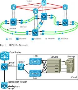
The IP/WDM network consists of two layers, the IP layer and the optical layer. In the IP layer, an IP router is used at each node to aggregate data traffic from access networks. Each IP router is connected to the optical layer through an optical switch. Optical switches are connected to optical fiber links where a pair of multiplexers/demultiplexers is used to multi-plex/demultiplex wavelengths [15]. Optical fibers provide the large capacity required to support the communication between IP routers. Transponders provide OEO processing for full wave-length conversion at each node. In addition, for long distance transmission, EDFAs are used to amplify the optical signal on each fiber. Fig. 1 shows the architecture of an IP/WDM network. Two approaches can be used to implement the IP/WDM net-work, namely, lightpath bypass and non-bypass. In the bypass approach, lightpaths are allowed to bypass the IP layer of in-termediate nodes eliminating the need for IP router ports, the most power consuming devices in the network, which signifi-cantly reduces the total network power consumption compared to the non-bypass approach. However, implementing such an ap-proach involves many technical challenges such as the need for long reach, low power optical transmission systems, limitations with the loss of electronic processing and as such the advantages electronic processing provides at intermediate nodes in terms of grooming, shared protection [16], and deep packet inspection. On the other hand, the forwarding decision in the non-bypass

Fig. 1. IP/WDM Network.

Fig. 2. Cloud architecture.

approach is made at the IP layer; therefore, the incoming light-paths go through OEO conversion at each intermediate node. The non-bypass approach is implemented in most of the current IP/WDM networks. In addition to the simple implementation, the non-bypass approach allows operators to perform traffic con-trol operations such as deep packet inspection and other analysis measures.

A number of papers in the literature have investigated the en-ergy efficiency of IP/WDM networks. The authors in [15] have shown that the lightpath bypass approach usually reduces the power consumption compared to the non-bypass approach as bypassing the IP layer at intermediate nodes reduces the num-ber of router ports, the major power consumers in IP/WDM networks. In [17], the authors focused on reducing the CO2 emission of backbone IP/WDM networks by introducing re-newable energy sources. In [18], a MILP model is developed to optimize the location of datacentres in IP/WDM networks as a means of reducing the network power consumption. In [19], energy-efficient IP/WDM physical topologies are investigated considering different IP/WDM approaches, nodal degree con-straints, traffic symmetry and renewable energy availability. In this paper we evaluate our proposed cloud models over a non-bypass IP/WDM network as non-non-bypass is still the most widely implemented approach.

core node, traffic will flow through the optical switch and core router on its way towards the core network. On the other hand if the users are located on the same node, the traffic will flow through the optical switch on its path towards the aggregation router where it will be routed to local users. The core/edge network power consumption of the second scenario is limited to the optical switch and aggregation router.

III. ENERGYEFFICIENTCONTENTDELIVERYCLOUD

A. Content Delivery Cloud MILP Model

Jointly optimizing content distribution for content providers (CPs) and traffic engineering for Internet service providers (ISPs) is studied in [20] from QoS perspective. The authors in [21] studied the same problem from energy point of view where ISP and CP cooperate to minimize energy. In [22], the authors compared conventional and decentralized server based content delivery networks (CDN), content centric networks (CCN), and centralized server based CDN using dynamic opti-cal bypass where they took popularity of content into account. In their conventional CDN model, content is fully replicated to all datacenters regardless of content popularity. They showed that CCN is more energy efficient in delivering the most popular content while CDN with optical bypass is more energy efficient in delivering less popular content.

In this section we introduce the MILP model developed to minimize the power consumption of the cloud content delivery service over non-bypass IP/WDM networks. Given the client requests, the model responds by selecting the optimum num-ber of clouds and their locations in the network as well as the capability of each cloud so that the total power consumption is minimized. The model also decides how to replicate content in the cloud according to its popularity so the minimum power possible is consumed in delivering content. A key difference between our content delivery model and the work done in the literature is the extensive study of the impact of content pop-ularity among different locations where we compare content replication schemes.

Below we re-introduce our model developed in [14] for com-pleteness. We assume the popularity of the different objects of the content follows a Zipf distribution, representative of the popularity distribution of several cloud content types such as YouTube and others [23] where the popularity of an object of rankiis given as follows:

P(i) =ϕ/i

whereP(i)is the relative popularity of the object of rankiand

ϕis

ϕ=

_N

i= 1 1 i

−1

.

We divide the content in our model into equally sized pop-ularity groups. A poppop-ularity group contains objects of similar popularity.

We define the following variables and parameters to represent the IP/WDM network:

Parameters:

N Set of IP/WDM nodes.

N mi Set of neighbors of node i.

|N| Number of IP/WDM nodes.

P rp Router port power consumption.

P t Transponder power consumption.

P e EDFA power consumption.

P Oi Power consumption of optical switch installed at

nodei∈N.

P md Multi/demultiplexer power consumption.

W Number of wavelengths per fiber.

B Wavelength bit rate.

S Max span distance between EDFAs.

Dm n Distance between node pair (m, n).

Am n Number of EDFAs between node pair (m, n). P U E n IP/WDM network power usage effectiveness. M A large enough number.

Δt Time granularity, which represents the evaluation period.

Variables (All are Nonnegative Real Numbers)

Cij Number of wavelengths in the virtual link(i, j). Lsd

ij Traffic flow between node pair (s, d) traversing

virtual link (i, j).

Wij

m n Number of wavelength channels in the virtual link

(i, j) traversing physical link (m, n).

Wm n Total number of used wavelengths in the physical

link (m,n).

Fm n Total number of fibers on the physical link (m,n). Qi Number of aggregation ports in router i.

Under the non-bypass approach, the total network power con-sumption is composed of [15], [18]:

1) The power consumption of router ports

i∈N

P rp·Qi+Prp·

m∈N

n∈N mm

Wm n.

2) The power consumption of transponders

m∈N

n∈N mm

P t·Wm n.

3) The power consumption of EDFAs

m∈N

n∈N mm

P e·Am n ·Fm n.

4) The power consumption of optical switches

i∈N P Oi.

5) The power consumption of multi/demultiplexers

m∈N

n∈N mm

P md·Fm n.

The content delivery cloud is represented by the following variables and parameters:

Parameters:

Ud Set of users in node d.

P G Set of popularity groups,{1. . .|P G|}.

P U E c Cloud power usage effectiveness.

S P C Storage power consumption.

S C Storage capacity of one storage rack in GB.

Red Storage and switching redundancy.

S P P GB Storage power consumption per GB,

S P P GB=S P C/S C.

S U tl Storage utilization.

P GSp Popularity group storage size, P GSp =

(S C/|P G|)·S U tl.

CS C Content server capacity.

CS EP B Content server energy per bit.

Sw P C Cloud switch power consumption.

Sw C Cloud switch capacity.

Sw EP B Cloud switch energy per bit, Sw EP B=

Sw P C/Sw C.

R P C Cloud router power consumption.

R C Cloud router capacity.

R EP B Cloud router energy per bit, R EP B=

R P C/R C.

Drate Average user download rate.

Pp Popularity of objectp(Zipf distribution). N Dd Node d total traffic demand, N Dd =

i∈UdDrate.

DP d Popularity group p traffic to node d, Dpd= N Dd·Pp.

Variables (All are Nonnegative Real Numbers)

δsdp δsdp = 1if popularity grouppis placed in node

sto serve users in noded, δsdp = 0otherwise.

LPsdp Traffic generated due to placing popularity group pin nodesto serve users in node d.

Lsd Traffic from cloudsto users in node d. Cups Cloudsupload capacity.

δsp δsp = 1 if cloud s stores a copy of popularity

groupp, δsp= 0otherwise.

Clouds Clouds = 1 if a cloud is built in node

s,Clouds = 0otherwise. CN Number of clouds in the network.

CSNs Number of content servers in cloud s. SwNs Number of switches in cloud s. RNs Number of routers in cloud s. StrCs Cloudsstorage capacity.

The cloud power consumption is composed of

1) The power consumption of content servers (SrvP C CD):

s∈N

Cups·CS EP B.

2) The power consumption of switches and routers (LAN P C CD):

s∈N

Cup_s·(Sw EP B·Red+R EP B).

3) The power consumption of storage(StP C CD):

s∈N

StrCs·S P P GB·Red.

The model is defined as follows:

Objective: Minimize

P U E n·

i∈N

P rp·Qi+P rp·

m∈N

n∈N mm

Wm n

+

m∈N

n∈N mm

P t·Wm n

+

m∈N

n∈N mm

P e·Am n·Fm n

+

i∈N P Oi+

m∈N

n∈N mm

P md·Fm n

+P U E c·

s∈N

Cups·CS EP B

+

s∈N

Cups·(Sw EP B·Red+R EP B)

+

s∈N

StrCs·S P P GB·Red

. (1)

Equation (1) gives the model objective which is to minimize the IP/WDM network power consumption and the cloud power consumption

Subject to:

1) Flow conservation constraint in the IP layer

j∈N:i=j

Lsd_ij − j∈N:i=j

Lsd_{j i} =

⎧ ⎨ ⎩

Lsd ifi=s

−Lsd ifi=d

0 otherwise

∀s, d, i∈N:s=d. (2)

Constraint (2) is the flow conservation constraint for IP layer. It ensures that the total incoming traffic is equal to the total out-going traffic for all nodes except for the source and destination nodes.

2) Virual link capacity constraint

s∈N

d∈N:s=d

Lsd_ij ≤Cij·B

∀i, j∈N:i=j. (3) Constraint (3) ensures that the traffic traversing a virtual link does not exceed its capacity.

3) Flow conservation constraint in the optical layer

n∈N mm

Wm nij −

n∈N mm

Wn mij = ⎧ ⎨ ⎩−

Cij ifm=i Cij ifm=j

0 otherwise

∀i, j, m∈N:i=j. (4)

4) Physical link capacity constraints

i∈N

j∈N:i=j

Wm nij ≤W ·Fm n

∀m∈N ∀n∈N mm. (5)

i∈N

j∈N:i=j

W_{m n}ij =Wm n

∀m∈N ∀n∈N mm. (6)

Constraints (5) and (6) represent the physical link capacity constraints. Constraint (5) ensures that the number of wave-length channels in virtual links traversing a physical link does not exceed the capacity of fibres in the physical link. Constraint (6) ensures that the number of wavelength channels in virtual links traversing a physical link is equal to the number of wave-lengths in that physical link.

5) Number of aggregation ports constraint

Qi = 1/B·

d∈N:i=d Lid

∀i∈N. (7) Constraint (7) calculates the number of aggregation ports for each router. We use relaxation in our model due to the large number of variables. However, as we are interested in power consumption, relaxation has a limited impact on the final re-sult as the difference will be within the power of less than one wavelength (router port and transponder) which is negligible compared to the total power consumption. The heuristics which produce comparable results provide independent verification for the model (and its relaxation), especially that the routing and placements in the heuristics follow approaches that are indepen-dent of the model.

6) IP/WDM network traffic

LPsdp =δsdp ·DP d

∀s, d∈N ∀p∈P G (8)

s∈N

LPsdp =DP d

∀d∈N ∀p∈P G. (9)

Lsd =

p∈P G LPsdp

∀s, d∈N. (10)

Cups =

d∈N Lsd

∀s∈N. (11) Constraint (8) calculates the traffic generated in the IP/WDM network due to requesting popularity grouppthat is placed in nodesby users located in noded. Constraint (9) ensures that each popularity group request is served from a single cloud only. We have not included traffic bifurcation where a user may get parts of the content from different clouds. This is a useful extension to be considered in future. Constraint (10) calculates

the traffic from the cloud in nodesand users in node d, to be used in constraints (2) and (7). Constraint (11) calculates each cloud upload capacity based on total traffic sent from the cloud.

7) Popularity groups locations

d∈N

δsdp ≥δsp

∀s∈N ∀p∈P G. (12)

d∈N

δsdp ≤M·δsp

∀s∈N ∀p∈P G. (13)

Constrains (12) and (13) ensure that popularity group pis replicated to cloudsif cloudsis serving requests for this pop-ularity group, whereM is a large enough unitless number to ensure thatδsp = 1when

d∈Nδsdp is greater than zero. 8) Cloud location and number of clouds

p∈P G

δsp ≥Clouds

∀s∈N. (14)

p∈P G

δsp ≤M·Clouds

∀s∈N. (15)

CN =

s∈N

Clouds. (16)

Constraints (14) and (15) build a cloud in location sif that location is chosen to store at least one popularity group or more, where M is a large enough unitless number to ensure thatClouds= 1when

p∈P Gδspis greater than zero.

Constraint (16) calculates total number of clouds in the net-work.

9) Cloud Capability

CSNs =Cups/CS C

∀s∈N. (17)

SwNs= (Cups/Sw C)·Red

∀s∈N. (18)

RNs=Cups/R C

∀s∈N. (19)

StrCs=

p∈P G

δsp·P GSp.

∀s∈N. (20)

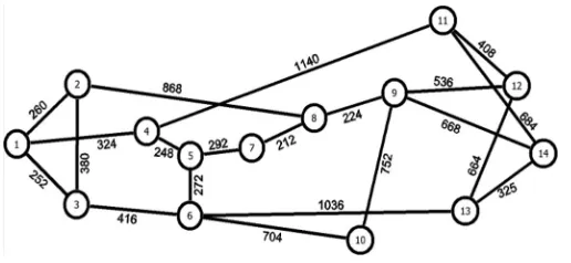
Fig. 3. The NSFNET network with link lengths in kilometer.

Fig. 4. Number of users versus time of the day.

switches (SwNs)is calculated considering redundancy.

Con-straint (20) calculates the storage capacity needed in each cloud based on the number of replicated popularity groups.

B. The Content Delivery Cloud Model Results

The NSFNET network, depicted in Fig. 3, is considered as an example network to evaluate the power consumption of the cloud content delivery service over IP/WDM networks. It has 14 nodes and 21 bidirectional links [15]. In this paper the network is designed considering the peak traffic to determine the maximum resources needed. However we still run the model considering varying levels of traffic throughout the day to optimally repli-cate content as the traffic varies to obtain the minimum power consumption. One point in the operational cycle (the point that corresponds to the peak demand) is strict network design where the maximum resources needed are determined. At every other point the optimization is a form of adaptation where resources lower than the maximum are determined and used to meet the demand.

In our evaluation users are uniformly distributed among the NSFNET nodes and the total number of users in the network fluctuates throughout the day between 200 k and 1200 k as shown in Fig. 4. The values in Fig. 4 are estimated, based on the data in [18]. The number of users throughout the day considers the different time zones within the U.S. [18]. The reference time zone in Fig. 4 is EST. We use the model to evaluate the power consumption associated with the varying number of users at the different times of the day, with a 2 h granularity.

Table I gives the input parameters of the model. The router ports power consumption and number of wavelength per fiber is based on [15], note that the power consumption of the IP

TABLE I

INPUTDATA FOR THEMODELS

router port takes into account the power consumption of the different shared and dedicated modules in the IP router such as the switching matrix, power module and router processor. The eight-slot CRS-1 consumes about 8 kW and therefore the power consumption of each port is given as 1 kW.

The ITU grid defines 73 wavelengths at 100 GHz spacing or alternatively double this number approximately at 50 GHz channel spacing. In more recent studies [29] we have adopted lower router power per port, 440 W, based on Alcatel-Lucent designs. Also a larger (>16) number of wavelengths per fiber is possible at 100 or 50 GHz spacing, however with super channels and the introduction of 400 Gb/s and envisaged 1 Tb/s and possibly flexigrid developments, the number of channels may fall. Also note that a larger number of wavelengths per fiber will reduce the number of fibers and hence EDFAs, but the power consumption of the latter is small. To facilitate comparison with previous studies we have adopted the figures in [15], [18]. Note that data rate of router ports is the same as the wavelength rate (40 Gb/s).

The energy per bit (EPB) in the table is capacity based as we base it on the maximum power and maximum rate of the server. However note that the model always attempts to fully utilize servers, see constraint (17) and switches off unused servers to minimize power consumption. The combination of these two operational factors results in EPB based on capacity being a good representation. The 5 Mbps average download rate is based on the results of a survey conducted in the U.S. in 2011 [27].

implement sophisticated water cooling [30] to small data centers with PUE as high as 3 [31]. We have adopted a PUE of 2.5 in this study for the small distributed clouds considered.

We divide the cloud content into 50 popularity groups which is a reasonable compromise between granularity and MILP model execution time. Note also that distributing the content into mul-tiple locations does not increase the power consumption of the cloud, i.e., the power consumption of a single cloud with all the content is equal to the total power consumption of multiple distributed clouds storing the same content without replication. The reason is that each server has an idle power; however, it is either switched ON (and through packing is operated near max-imum capacity) if needed or switched OFF. The cloud is made up of a large number of servers (200 for example, see Fig. 10). The cloud power consumption therefore increases with good granularity in steps equal to the power consumption of a single server. This leads to a staircase (with sloping stairs) profile of power versus load and with the very large number of steps, the profile is almost linear. This form of power management means that placing a given piece of content in different clouds amounts to the same power consumption approximately. We also assume similar type of equipment and PUE, hence we do not assume a fixed power component associated with placing a cloud in cer-tain location. We also assume that underutilized storage units, switches, and routers) in the cloud are switched OFF or put in low power sleep mode. Note that savings are averaged over the 12 time points of the day (24 h). The metrics used are average savings over 24 h. These are the average network power saving, average cloud power saving and average total power saving.

Note that the variables specified above (with the exception of binary variables) take values that are dictated by the num-ber of users, their data rates, content popularity and scenario considered.

We compare the following different delivery schemes: 1) Single cloud: Users are served by single cloud optimally

located at node 6 as it yields the minimum average hop count. This scenario is obtained by setting the total number of clouds to 1, i.e., constraint (16) becomes

CN=

s∈N

Clouds= 1.

We consider two schemes in this model:

a) No power management (SNPM): The cloud and the network are energy inefficient where different com-ponents are assumed to consume 80% of their max-imum power consumption at idle state.

b) Power management (SPM): The cloud and the net-work are energy efficient where underutilized com-ponents are powered off or put into deep sleep at off-peak periods.

2) Max number of clouds with power management: A cloud is located at each node in the network, i.e. the network contains 14 clouds. In this case the total number of clouds is set to 14, i.e., constraint (16) becomes

CN =

s∈N

Clouds = 14.

We consider three schemes in this model

a) Full replication (MFR): Users at each node are served by a local cloud with a full copy of the con-tent. This scheme is obtained by setting the number of popularity groups to 1, i.e.,|P G|= 1.

b) No replication (MNR): The content is distributed among all the 14 clouds without replication. This scheme is obtained by ensuring that the total number of replicas(δsp)does not exceed the original number

of popularity groups(|P G|):

p∈P G

s∈N

δsp =|P G|.

c) Popularity based replication (MPR): The model op-timizes the number and locations of content replicas among all the 14 clouds based on content popularity. 3) Optimal number of clouds with power management: The number and location of clouds are optimized. We consider three schemes of this scenario:

a) Full replication (OFR): Each cloud has a full copy of the content. This scheme is obtained by setting

|P G|= 1.

b) No replication (ONR): Content is distributed among the optimum clouds without replication. This scheme is obtained by setting

p∈P G

s∈N

δsp =|P G|.

c) Popularity based replication (OPR): The number and locations of content replicas are optimized based on content popularity.

We reduce the popularity group size to 20% of the size con-sidered in the results of [14], i.e.,PGSp =0.756TB. A single

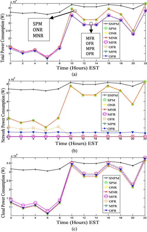
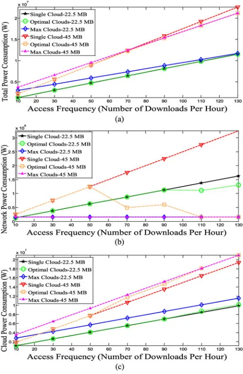
download rate of 5 Mb/s is used for the two cases of file size. The two file sizes may for example correspond to two movies of different length and/or different resolution. At a constant user rate the time taken to download the larger file (before playing in this case) is longer. The smaller popularity group size represents a cloud scenario where music, for instance, is more popular than movies. Fig. 5(a) shows the total power consumption of the dif-ferent schemes while Fig. 5(b) and (c) shows the network and cloud power consumptions, respectively.

Fig. 5. (a) Total power consumption. (b) IP/WDM network power consump-tion. (c) Cloud power consumpconsump-tion.

that the traffic is uniformly distributed among the nodes. Note that this choice of the reference case is conservative. We could have chosen the reference case as a single cloud, but optimally placed to minimize delay or network CAPEX as is currently done, in which case the energy savings as a result of our work will be higher.

We also investigate the other extreme scenario represented by the MFR scheme where content is fully replicated into all possible locations (14 nodes of the NSFNET). At the network side (see Fig. 5(b)), the MFR saves 99.5% of the network power consumption as all requests generated in a node are served locally. The other 0.5% of the power consumption is associated with the optical switch shown in Fig. 2. However, having a cloud with full content at each node, especially with large popularity group size, significantly increases the cloud power consumption due to storage. Therefore the MFR scheme is not efficient if storage power consumption continues to dominate the power consumption of datacenters, for instance, we have shown in [14] that MFR cloud power consumption even exceeds the SNMP

cloud power consumption at peak periods of the day, such as at 10:00, 16:00 and 22:00.

Despite their different approaches in optimizing content de-livery, the MNR, ONR and SPM schemes have similar total power consumption. In terms of the cloud power consumption, the three schemes produce the lowest power consumption as content is not replicated and as mentioned above distributing the content into multiple locations does not increase the power consumption. In the following we discuss the network power consumption of the different schemes.

The ONR scheme finds the optimal number of clouds required to serve all users from a single copy of the content, where dif-ferent popularity groups are migrated to difdif-ferent clouds based on their popularity. However, our results show that the ONR scheme selects to serve users using a single cloud located at node 6, i.e., ONR imitates the SPM scheme. This is because distributing the content into multiple clouds without replicating it results in higher network power consumption. For instance, if the ONR scheme decides to build two clouds one at node 1 (far left end of NSFNET) and the other at node 12 (far right end of NSFNET), then users at nodes located at the left end of the network will have to cross all the way to the right end of the network to download some of their content from cloud at node 12 as we do not allow this content to be replicated into the cloud in node 1, and vice versa for users located at nodes at the right end of the network asking for content only available at node 1. However, if all popularity groups are kept in node 6 which is the node that yields the minimum average hop count to differ-ent nodes in the network (this will be shown later in Section III-C), then the power consumed in the network to download content will be minimized, resulting in 37% saving in both total and network power consumption compared to SNPM, similar to SPM.

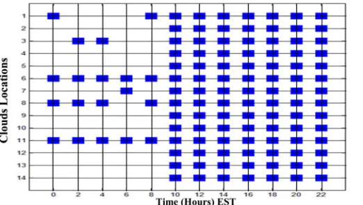
Fig. 6. OFR powered ON clouds at different times of the day.

ONR and MNR still follow the SPM scheme and centralize the content in one cloud at node 6, as observed in [14]. Therefore centralizing the content is the optimum solution if content is not allowed to be replicated regardless of content size.

As already observed, serving content locally by enforcing replication in all the 14 locations (MFR scheme) yields the highest cloud power consumption and the lowest network power consumption. In the OFR scheme we investigated the impact of removing the constraint on the number of clouds; so the model is free to choose the optimal number of clouds that have a full copy of the content. The OFR scheme manages to reduce the total number of clouds from 14 to 6 at off-peak periods of the day (between 00:00 and 08:00). These clouds are switched on and off according to the traffic variation as seen in Fig. 6. However, at peak periods (between 10:00 and 22:00) the OFR scheme converges to MPR scheme and builds clouds at all nodes as the power saved in the network is higher than the power lost in storage replication. OFR achieves significant power savings at the network side of 92% compared to the SNPM scheme, a saving higher than what is achieved by the SPM, ONR and MNR as the content is fully replicated to optimally located clouds. Eventually, the OFR scheme increases the total power saving compared to the SPM, ONR and MNR schemes, where the cloud in node 6 is mainly used, from 37% to 42.5% compared to SNPM, which is also slightly higher saving compared to MFR scheme due to deploying fewer clouds at off-peak periods.

From the discussion above it can be seen that the savings achieved by the OFR scheme are limited by the constraint on the content replication granularity where all content is replicated to a certain location if a cloud is created in that location. The question raised next is how much can the limits of power saving be pushed if the constraints on both the number of clouds and content replicated at each cloud are removed. This approach is implemented by the OPR scheme. The results in Fig. 5 indicate that the OPR scheme provides solutions with the lowest total power consumption.

The OPR, MPR and OFR schemes in this case have similar power consumption to the MFR scheme (43% total power sav-ings compared to SNPM) which implies that the three schemes tend to replicate the majority of the content in all the 14 clouds

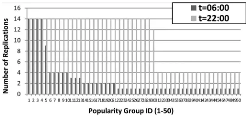
Fig. 7. Popularity groups placement under the OPR scheme at 06:00 and 22:00.

most of the time due to the small storage power cost as shown in Fig. 5(c).

Fig. 5(b) shows that the network power savings for the dif-ferent models follow a similar trend to that in Fig. 5(a). At the network side, the OPR, MPR, OFR and MFR schemes save 92–99.5% of the network power consumption compared to the SNPM scheme while the SPM, ONR and MNR schemes save 37% of the network power consumption. Despite their similar average network power saving, OPR and OFR have different behaviour in saving power at the network side. OPR maintains the network power at the lowest level at all times by powering on the optimum number of clouds with the optimum content. However, OFR is less flexible as all the powered on clouds have to have a full copy of the content. Therefore OFR powers on only four clouds at low load and consumes higher network power while behaving as MFR and consuming power only in optical switches at high loads (10:00 to 22:00) by powering on 14 clouds (see Fig. 6), resulting in a daily average network power consumption similar to the OPR scheme.

Fig. 8. Total number of replications per popularity group under the OPR scheme.

Fig. 9. Number of popularity groups replicated at each cloud under the OPR scheme.

it will be replicated (black circle) to more clouds as this will result in serving more requests locally and therefore reducing the network power consumption. At 06:00, most of the content is kept in node 6, while at 22:00, more popularity groups are replicated into more clouds as under higher loads the power consumption of the cloud is compensated by higher savings in the network side. Compared to the results of [14], Fig. 7 shows that OPR tends to replicate more content to more clouds due to lower power consumption of storage, especially that we fixed the average download rate at 5 Mbps. As content is equally pop-ular among all users and users are uniformly distributed among nodes, OPR will replicate the most popular content into all the 14 nodes most of the day. Therefore OPR has similar power effi-ciency to the MPR where content is optimally replicated among all the 14 clouds based on its popularity.

Fig. 8 shows the total number of replicas per popularity group for the OPR scheme, obtained by summing the black circles for each popularity group in Fig. 7. At low demand, the number of replications follows a Zipf distribution. However, at high de-mand (at 22:00), the scheme does not follow a Zipf distribution in replicating content as the high demand and the low power cost of storage allow the majority of the popularity groups to be replicated into all the nodes.

Fig. 9 shows the total number of popularity groups replicated at each built cloud, obtained by summing the black circles in Fig. 7 for each cloud; i.e., Fig. 9 reflects the relative cloud size built at each node. At low demand periods (06:00) most of the content is replicated to the cloud in node 6 only, while at peak period (time 22:00) fewer popularity groups are replicated to

Fig. 10. Number of powered on servers in each cloud under the OPR scheme.

TABLE II

THEPOWERSAVINGSGAINED BY THEDIFFERENTCONTENTDELIVERY CLOUDSSCENARIOSCOMPARED TO THESNPM SCENARIO

the cloud in node 6 as the high network power savings at peak period justify replicating the content to more clouds instead of having a single copy in a centralized cloud. Due to the low power cost of storage, content is replicated to more clouds at both high and low loads compared to the larger popularity group results in [14].

Fig. 10 shows the number of servers powered on at each cloud att=06:00 andt=22:00. The number of servers powered on at each cloud at a certain time is proportional to the size of content replicated to the cloud given in Fig. 9. Fewer servers are powered on at node 6 at both times compared to the results of [14] as more requests are served from other clouds due to low storage cost. Note that the number of switches and routers at each cloud follows a similar trend to that of the number of servers.

From the results above it is observed that OPR is always the best scenario for content delivery. OPR converges to a single cloud scenario for content of larger size at low demand periods while it fully replicates contents at all network locations for content of smaller size at high demand periods. OPR can be realized either by replicating popular content to the optimized locations and continuously replacing it as the popularity changes throughout the day; or by replicating all the content to all clouds and only switching on the hard disks storing the content with the highest popularity, selected by the model at each location. The latter storage management approach saves power in the network side; however, it needs knowledge of content popularity to assign separate hard disks to different popularity groups.

C. DEER-CD: Energy Efficient Content Delivery Heuristic for the Cloud

As OPR is the most energy efficient scheme among the dif-ferent schemes investigated, in this section we build a heuristic (DEER-CD) to mimic the OPR model behaviour in real time. We need to build a mechanism to allow the cloud management to react to the changing network load by replicating the proper content to the optimum locations rather than deciding an aver-age replication scheme that might not fit well with different load patterns throughout the day. The DEER-CD heuristic involves two phases of operation:

1) Offline phase: Each node in the network is assigned a weight based on the average number of hops between the node and the other nodes and the traffic generated by the node, i.e., the number of users in the node and their download rate. The weight of node s,N Ws,is given as

N Ws =

d∈N

Ud· Drate ·Hsd (21)

where Ud is the number of users in node d andHsd is the

minimum number of hops between node pair (s, d).

As the network power consumption is proportional to the amount of content transiting between nodes and the number of hops travelled by the content, nodes of lower weight are the optimum candidates to host a cloud. Equation (21) can be pre-calculated as it relies on information that rarely changes throughout the day such as the physical topology, average users population and download rate. We construct a sorted list of nodes from lowest to highest weight and use this list to make cloud placement decisions. In the absence of our sorted list approach, an exhaustive search is needed where a PG can be allocated to a single node leading to|N|(number of nodes) combinations being evaluated for network energy efficiency. In addition the PG can be allocated to two nodes leading to the evaluation of

|N| ·(|N| −1) combinations, and therefore in total this ex-haustive search, which we totally avoid, requires|_iN_{= 1}| _(|N|N_|−|!_i)! placement combinations to be assessed. Our sorted list reduces this search to the evaluation of |N| combinations only. For NSFNET with|N| = 14this is a complexity reduction by a factor of 1.6×1010_{. Furthermore using a 2.4 GHz Intel Core} i5 PC with 4 GB Memory, the heuristic took 1.5 min to evaluate the DEER-CD results.

In our scenario the users are uniformly distributed over all nodes and they all have the same average download rate of 5 Mbps. Therefore the nodes’ ranking is mainly based on the average number of hops. The list of ordered nodes based onCs

from the lowest to the highest is as follows:

LIST={6, 5, 4, 3, 7, 9, 13, 10, 11, 12, 14, 1, 8, 2}.

To place a given popularity group in one cloud, node 6 is the best choice as it has the minimum weight. If the model decides to have two replicas of the same popularity group, then they will be located at nodes{6, 5}. Higher numbers of replicas are located similarly by progressing down the list and replicating content in a larger ordered subset of the set above. We call each subset of the list a placement(J). Therefore, DEER-CD will only have 14 different placements for each popularity group to choose from,

Fig. 11. The DEER-CD heuristic pseudo-code.

which dramatically minimizes the number of iterations needed to decide the optimal placement for each popularity group.

2) Online phase: In this phase, the list generated from the offline phase is used to decide the placement of each popularity group. Fig. 11 shows the pseudo code of the heuristic.

For each popularity group, the heuristic calculates the total power consumptionTPCiJ associated with placing each

pop-ularity groupi∈P Gin each placement,J ⊆LIST. The total power consumption is composed of network power consump-tionNPCiJ and the cloud power consumptionCPCiJ, at each

placement J. Each cloud location candidate in the placement,

s∈J(loop(a)), is assigned to serve nodes according to the mini-mum hop count (loop (b)).(LiJ sd)is the traffic matrix generated

by placing popularity groupiin the set of nodessthat are spec-ified by the associated placementJ, ddenotes the set of other nodes in the network where users are requesting files in popu-larity groupi. We use multi hop non-bypass heuristic developed in [15] to route the traffic between nodessanddand calculate the network power consumption that is induced due to cross traffic between the nodes associated with each placement (14 possible placements) for each popularity group (loop (c)). The total power consumption is calculated and the placement asso-ciated with the lowestTPCiamong the 14 possible placements

is selected to replicate the popularity group (loop (d)).

Fig. 12. (a) Total power consumption of the DEER-CD heuristic. (b) IP/WDM network power consumption of the DEER-CD heuristic. (c) Cloud power con-sumption of the DEER-CD heuristic.

it is able to carry out a complete network design and a complete cloud design which is different from dynamic operation over an existing cloud and an existing network.

Note that our heuristic in its current form does not consider the capacity constraints explicitly (such as the number of installed fibres and other network elements) as we consider designing the network for peak traffic(t =22:00) first and running the heuristic at times where the traffic is less than the peak traffic (see Fig. 4). The heuristic can however be easily updated to work in a capacitated network.

Fig. 12(a) shows the total power consumption for the DEER-CD heuristic, while Fig. 12(b) and (c) show the IP/WDM net-work and cloud power consumptions, respectively, also under the DEER-CD heuristic. For the larger size popularity group scenario, the OPR model and the DEER-CD heuristic achieve comparable network power savings of 72% and 70%, respec-tively, compared to SNPM scheme. Also the cloud and total power savings achieved by the OPR model are maintained at 34% and 40%, respectively. This is due to the almost identi-cal popularity groups’ placement by the model and heuristic. A

Fig. 13. Total number of replications per popularity group for DEER-CD (PGSp=3.78TB).

Fig. 14. Total number of replications per popularity group for DEER-CD(PGSp=0.756TB).

TABLE III

OPTIMIZATIONGAPSBETWEEN THEDEER-CD HEURISTIC ANDMILP

Similar observation is noticed for the smaller popularity group where the DEER-CD heuristic maintains the network, cloud and total power savings of 92%, 35% and 43%, respectively, achieved by the OPR model.

optimization gaps between the DEER-CD heuristic and the OPR model for both larger and smaller popularity group sizes at low and high traffic.

IV. ENERGYEFFICIENTSTORAGE AS ASERVICE

StaaS can be viewed as a special case of the content delivery service where only the owner or a very limited number of autho-rized users have the right to access the stored content. Dropbox, Google Drive, Skydrive, iCloud, and Box are examples of cloud based storage. In energy efficient StaaS, all content is stored in one or more central locations and dynamically migrated to loca-tions in proximity of its owners to minimize the network power consumption. The content can be migrated, content migration, however, consumes power at the IP/WDM network as well as in the servers and internal LAN of the clouds. Therefore, StaaS should achieve a trade-off between serving content owners di-rectly from the central cloud/clouds and building clouds near to content owners. Upon registration for StaaS, users are granted a certain size of free storage (Quota). DropBox [32], for instance, grants its users 2 GB. Different users might have different levels of utilization of their StaaS quota as well as different files ac-cess frequency. Large file acac-cess frequency has two meanings: either one user highly accesses it or many authorized users have low/moderate access frequency to the same file.

A. StaaS MILP Model

We extend the model in Section III-A to capture the distinct features of StaaS. As only the owner or a very limited number of authorized users have the right to access the stored content, the concepts of popularity and replication do not apply to StaaS. In addition to the parameters and variable defined in Section III-B, we define the following:

Parameters:

F req Average file download frequency per hour.

Dsize Average file size in Gb.

Rate Average user rate per second, whereRate= 2· F req·Dsize/3600.

N Dd Node d total traffic demand, N Dd =

i∈Ud Rate.

Quota Users storage quota in Gb.

SUi Storage Quota utilization of user i.

α 1 or 2.

Variables (All are Nonnegative Real Numbers)

ITcd Traffic between the central cloud and cloud in

nodeddue to content migration.

CUsd Traffic from the cloud in nodesto users in node

d.

πsd πsd= 1if cloudsserves users in noded, πsd = 0

otherwise.

Lsd Total traffic between node pair (s, d).

Note that the average user rate, Rate, substitutes Drate in Section III-A and is calculated by dividing total amount of data sent and received which (are measured in Gb, and equal to2· Freq·Dsize) over one hour by number of seconds in one hour as users need to download the full file before editing and need

to upload the full file after finishing (or intermediately). Waiting is not desirable and the file access frequency dictates the data rate. The factor of 2 is introduced to represent the fact that users usually re-upload their files back to the cloud after downloading and processing them.

The objective of the model in Section III-A applies to the StaaS model, as well as constraints (1)–(7), (17)–(19). The fol-lowing additional constraints are introduced:

1) Clouds to users traffic

s∈N

CUsd =N Dd

∀d∈N (22)

M ·CUsd≥πsd

∀s, d∈N (23)

CUsd≤M ·πsd

∀s, d∈N (24)

CUcd=N Dd · ⎛

⎝1−

b∈N:b=c Cloudb

⎞ ⎠.

∀d∈N:d=c (25) Constraint (22) ensures that the traffic demand of all users in each node is satisfied. Constraints (23) and (24) decide whether a cloud serves users in node d or not, where M is a large enough number, with units of 1/Gb/s and Gb/s in (23) and (24), respectively, to ensure thatπsd= 1whenCUsd is greater than

zero. Constraint (25) sets the traffic between the central cloud and users in other nodes to 0 if those users have a nearby cloud to download their content from.

2) Clouds locations

M.

d∈N

CUsd ≥Clouds

∀s∈N (26)

d∈N

CUsd ≤M ·Clouds.

∀s∈N (27) Constraints (26) and (27) build a cloud in location sif that location is selected to serve the requests of users of at least one noded, whereM is a large enough number, with units of 1/Gb/s and Gb/s in (26) and (27), respectively, to ensure that Clouds = 1when

d∈N CUsdis greater than zero

3) Clouds storage capacity

StrCs =

d∈N

i∈Ud

πsd·Quota·SUi·Red.

4) Inter clouds traffic:

ITcd=

i∈Ud

Cloudd ·Quota·SUi/(3600·Δt).

∀d∈N :d=c (29) Constraint (29) calculates the content migration traffic be-tween the central cloud and local clouds. The factor ofΔtin the denominator scales the power consumption down to be consis-tent with our evaluation period ofΔthours.

5) Total traffic between nodes and clouds upload capacity

Lsd =CUsd+ITsd

∀s, d∈N (30)

Cup_s =

d∈N

(Lsd+α·ITsd).

∀s∈N (31) Constraint (30) calculates the total traffic between node pair (s, d) as the summation of the inter cloud traffic and clouds to users traffic. Constraint (30) substitutes constraint (10) in calculating network traffic. Constraint (31) calculates clouds upload capacity which includes the clouds to users traffic and the clouds inter traffic when s=c. The factorαis set to 2 if we are interested in total power consumption, as the receiving local cloud will consume similar power in its servers and internal LAN to the central sending cloud during migration. However, it is set to 1 if we are only interested in the actual clouds upload capacity and capability calculated by constraints (17)–(19). In this section we setα= 2as we are interested in power consumption.

B. StaaS Model Results

The NSFNET network, the users’ distribution and input pa-rameters discussed in Section III-C are also considered to eval-uate the StaaS model. Node 6 is optimally selected based on the insights of Section III to host one central cloud.

We analyze 1200 k users uniformly distributed among net-work nodes which correspond to time 22:00 in Fig. 4. Power consumption calculation is averaged over the range of access frequencies considered (10 to 130 downloads per hour).

We analyse three different schemes to implement StaaS: 1) Single cloud: Users are served by the central cloud only. 2) Optimal clouds: Users at each node are served either from

the central cloud or from a local cloud by migrating content from the central cloud.

3) Max clouds: Users at each node are served by a local cloud.

We evaluate the different schemes considering two file sizes of 22.5 MB and 45 MB and a user storage quota of 2 GB.

Note that the file sizes reflect content of high resolution im-ages or videos. Files of smaller sizes will result in low network traffic that will not justify replicating content into local clouds. Users’ storage utilization SUi is uniformly distributed

be-tween 0.1 and 1.

Fig. 15(a) shows the total power consumption versus the con-tent access frequency while Fig. 15(b) and (c) decompose it into

Fig. 15. (a) Total power consumption of StaaS. (b) IP/WDM network power consumption of StaaS. (c) Cloud power consumption of StaaS.

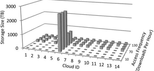
Fig. 16. Power-on clouds storage size versus content access frequency for the StaaS optimal scheme (45 MB file size).

On the network side, the Max Clouds scheme has the lowest network power consumption, saving 67% and 83% of the net-work power consumption compared to the Single Cloud scheme considering the 22.5 MB and the 45 MB average file size, re-spectively. This is because all users are served locally and the IP/WDM network power consumption is only due to content migration from the central cloud. However, this saving is at the cost of high power consumption inside the clouds to migrate content, resulting in an increase of 28% and 19% in the cloud power consumption for the 22.5 and 45 MB cases, respectively, as shown in Fig. 15(c).

For the 22.5 MB file size scenario, limited total and network power savings are obtained by the optimal clouds scheme com-pared to the single cloud scheme (0.1% total and 5% network power saving) as shown in Fig. 15(b). On the other hand, for the 45 MB file size scenario, more total and network power savings are obtained by the Optimal Cloud scheme compared to the Single Cloud scheme (2% total and 48% network power saving) as shown in Fig. 15(b).

Fig. 16 shows the variation in the number and size of clouds with the content access frequency for the 45 MB file size. As the content access frequency increases, migrating content from the central cloud to local clouds becomes more energy efficient compared to delivering content directly from the central cloud and therefore more clouds are needed to serve users locally. Note that the storage size in Fig. 16 represents the powered-on storage. This results in decreased storage size of the central cloud with higher content access frequency as shown in Fig. 16. Fig. 16 also shows that other clouds have almost similar storage size, at high access rates, due to the uniform distribution of users in the network.

V. VM PLACEMENTOPTIMIZATION

Machine virtualization provides an economical solution to efficiently utilize the physical resources, opening the door for energy efficient dynamic infrastructure management as high-lighted by many research efforts in this field. The authors in [33] studied the balance between server energy consumption and net-work energy consumption to present an energy aware joint VM placement inside datacenters. The authors in [34] proposed the use of multiple copies of active VMs to reduce the resource requirement for each copy of the VM by distributing the

incom-ing requests among them to increase the energy efficiency of the consolidation and VM placement algorithm. They consid-ered heterogeneous servers in the system and used a two dimen-sional model that considers both computational and memory bandwidth constraints. The authors in [35] proposed a MILP formulation that virtualizes the backbone topology and places the VMs in several cloud hosting datacenters interconnected over an optical network with the objective of minimizing power consumption.

In this section we optimize the placement of VMs in IP/WDM networks to minimize the total energy consumption. We con-sider different VM distribution schemes. In our analysis, a VM is defined as a logical entity created in response to a service request by one or more users sharing that VM. A user request is defined by two dimensions: (i) the CPU utilization (normalised workload) of the VM and (ii) the traffic demand between the VM and its user. In this section we use the terms CPU utilization and normalised workload interchangeably.

A. Cloud VM Placement MILP Model

We develop a MILP model to optimize the number, and lo-cation of clouds and optimize the placement of VMs within the clouds as demands vary throughout the day to minimize the network and clouds power consumption. The model considers three VM placement schemes:

1) VM replication: More than one copy of each VM is al-lowed in the network.

2) VM migration: Only one copy of each VM is allowed in the network. We assume that the internal LAN capacity inside datacenters is always sufficient to support VM migration. 3) VM slicing: The incoming requests are distributed among different copies of the same VM to serve a smaller number of users as proposed in [34]. We call each copy a slice as it has less CPU requirements. As VMs with small CPU share might threaten the SLA, we enforce a limit on the minimum size of the VM CPU utilization. Unlike [34] where CPU and memory bandwidth are considered, we consider the CPU and traffic dimensions of the problem where each slice is placed in a different cloud rather than in different server inside the same cloud.

In addition to the variables in Section III-A, we define the following variables and parameters:

Parameters:

V M Set of virtual machines.

Uv Set of users requesting VMv. N V M Total number of virtual machines.

Pm ax Maximum power consumption of a server.

Wm ax Maximum normalised workload of a server.

∇ Server energy per bit,∇=Pm ax/Wm ax.

Wv Total normalised workload ofV M v.

Ddv Traffic demand from VM v to node d, Ddv =

i∈Ud:i∈UvDrate.

M inW Minimum allowed normalised workload per VM.

Variables (All are Nonnegative Real Numbers)

Lsdv Traffic demand from VMvin cloudsto node d.

CWs Total normalised workload of Cloud s.

Wsv Normalised workload of the slice of VM v in

node s.

P SNs Number of processing servers in cloud s.

The power consumption of the cloud considering the machine virtualization scenario is composed of

1) The power consumption of servers(SrvP C V M)

s∈N

∇ ·CWs.

2) The power consumption of switches and routers (LAN P C V M)

s∈N

Cups·(Sw EP B·Red+R EP B).

Note that we do not include the storage power consumption in our models. Although the server power consumption is a func-tion of the idle power, maximum power and CPU utilizafunc-tion [36], for large number of servers, taking only∇=Pm ax/Wm axas the server EBP to calculate its power consumption yields very close approximation as the difference will be only in last powered on server. Note that a cloud is composed of a large number of servers and through “packing,” each server in our case is either as close to fully utilized as possible or is off. In such a case “idle power plus linear increase in power with load” is equivalent to “linear increase in power with load” as both servers are either operated near the peak or are off and the peak powers are iden-tical. For the overall cloud either a single server (or more gen-erally a very small minority of servers) may be partially loaded. Therefore for a cloud made up of a large number of highly used servers (unused servers are turned off), the power con-sumption increases in proportion to load approximately. Note that if servers are not fully packed, this approximation becomes less accurate. This warrants further investigation, however our approach is followed in the literature [28]. As for the content delivery model, we also assume here that other storage and network elements have similar power management as servers.

The model is defined as follows: Objective: Minimize

P U E n·

i∈N

P rp·Qi+P rp·

m∈N

n∈N mm

Wm n

+

m∈N

n∈N mm

P t·Wm n

+

m∈N

n∈N mm

P e·Am n·Fm n

+

i∈N P Oi+

m∈N

n∈N mm

P md·Fm n

+P U E c·

s∈N

∇·CWs+

s∈N

Cup_s·(Sw EP B·Red

+R EP B)

. (32)

Subject to 1) VMs demand

s∈N

Lsdv =Ddv

∀d∈N ∀v∈V M . (33)

Constraints (33) ensures that the requests of users in all nodes are satisfied by the VMs placed in the network.

2) VMs locations

M·

d∈N

Lsdv ≥δsv

∀s∈N ∀v∈V M (34)

d∈N

Lsdv ≤M·δsv

∀s∈N ∀v∈V M . (35)

Constraints (34) and (35) replicate VMvto cloudsif cloud

sis selected to serve requests forvwhereM is a large enough number, with units of 1/Gb/s and Gb/s in (34) and (35), respec-tively, to ensure thatδsv = 1when

d∈N Lsdv is greater than zero.

3) Clouds locations

v∈V M

δsv ≥Clouds

∀s∈N (36)

v∈V M

δsv ≤M·Clouds.

∀s∈N (37) Constraints (36) and (37) build a cloud in locations if the location is selected to host one or more VMs where M is a large enough unitless number to ensure thatClouds= 1when

v∈V Mδsv is greater than zero.

4) Total cloud normalised workload for replication and mi-gration schemes

CWs =

v∈V M

δsv·Wv.

∀s∈N (38) Constraint (38) calculates the total normalised workload of each cloud by summing its individualV M snormalised work-loads.

5) VM migration constraint

s∈N

δsv = 1

∀v∈V M . (39)

Constraint (39) is used to model the VM migration scenario where only one copy of each VM is allowed.

s∈N

Wsv =Wv

∀v∈V M (40)

Wsv≥M inW ·δsv

∀s∈N ∀v∈V M (41)

Wsv≤M ·δsv

∀s∈N ∀v∈V M (42)

CWs =

v∈V M Wsv

∀s∈N. (43) Constraints (40)–(43) are used to model the VM slicing sce-nario. Constraint (40) ensures that the total normalised workload of all slices is equal to the original VM normalised workload before slicing. Constraints (41) and (42) ensure that the loca-tions of the slices of a VM are consistent with those selected in constraints (34) and (35) and also they ensure that the slices nor-malised workload does not drop below the minimum allowed normalised workload per slice whereMis a large enough num-ber, with units of %, to ensure thatδsv = 1whenWsvis greater

than zero. Constraint (43) calculates the work load of each cloud by summing the load of the slices of the different VMs hosted by the cloud.

7) Single cloud scheme constraint

s∈N

Clouds = 1. (44)

Constraint (44) is used to model the single cloud scheme which is used as our benchmark to evaluate the power savings achieved by the different VM distribution schemes.

8) Number of processing servers

P SNs =CWs/Wm ax

∀s∈N. (45) Constraint (45) calculates the number of processing servers needed in each cloud. The integer value is obtained using the ceiling function.

B. Cloud VM Model Results

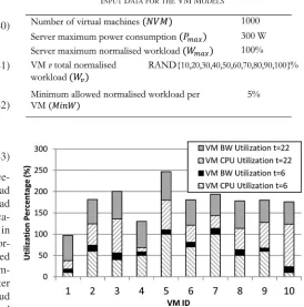
The VM placement schemes are evaluated considering the NSFNET network and the users distribution discussed in Section III-B. In addition to the input parameters in Table I, the VM model considers the parameters in Table IV. To reflect various users’ processing requirements and represent different types of VMs, we uniformally assign normalised workloads to VMs from the set given in Table IV.

Fig. 17 shows the server CPU and network bandwidth uti-lization of 10 VMs at two times of the day (06:00 and 22:00). Note that network utilization is calculated by assuming a 10 Gb/s servers’ interface speed and users traffic rates are kept at 5 Mbps as in Section III.

In a practical cloud implementation the CPU normalised workload needed is estimated by the cloud provider based on

TABLE IV

INPUTDATA FOR THEVM MODELS

Fig. 17. Sample VMs CPU and network utilization.

users’ requirements. Instead of starting with users requests for VMs and assigning them to VMs, we simplify the generation of CPU normalised workload by considering a set of 1000 VMs (limit of what MILP can handle) of different types and assign each VM a uniformly distributed normalised workload between 10% and 100% of the total CPU capacity. We then randomly and uniformly assign each VM to serve a number of users. This approach is less complex to analyze in terms of number of vari-ables and it captures the same picture. This can be understood by noting that a cloud provider will assign the incoming re-quests to a given VM according to its specialization up to a certain maximum normalised workload. This results in a distri-bution of VM normalised workloads and an assignment of users (from different nodes) to a VM which is what our approach also achieves.