This is a repository copy of Combinatorial optimization with 2-joins.
White Rose Research Online URL for this paper:
http://eprints.whiterose.ac.uk/74344/
Article:
Trotignon, N and Vuskovic, K (2012) Combinatorial optimization with 2-joins. Journal of
Combinatorial Theory: Series B, 102 (1). 153 - 185 . ISSN 0095-8956
https://doi.org/10.1016/j.jctb.2011.06.002
Reuse
See Attached
Takedown
If you consider content in White Rose Research Online to be in breach of UK law, please notify us by
Combinatorial optimization with 2-joins
Nicolas Trotignon∗ and Kristina Vuˇskovi´c†
June 1, 2011
Abstract
A 2-join is an edge cutset that naturally appears in decomposition of several classes of graphs closed under taking induced subgraphs, such as perfect graphs and claw-free graphs. In this paper we construct com-binatorial polynomial time algorithms for finding a maximum weighted clique, a maximum weighted stable set and an optimal coloring for a class of perfect graphs decomposable by 2-joins: the class of perfect graphs that do not have a balanced skew partition, a 2-join in the complement, nor a homogeneous pair. The techniques we develop are general enough to be easily applied to finding a maximum weighted stable set for another class of graphs known to be decomposable by 2-joins, namely the class of even-hole-free graphs that do not have a star cutset.
We also give a simple class of graphs decomposable by 2-joins into bipartite graphs and line graphs, and for which finding a maximum stable set is NP-hard. This shows that having holes all of the same parity gives essential properties for the use of 2-joins in computing stable sets.
AMS Mathematics Subject Classification: 05C17, 05C75, 05C85, 68R10 Key words: combinatorial optimization, maximum clique, minimum stable set, coloring, decomposition, structure, 2-join, perfect graphs, Berge graphs, even-hole-free graphs.
∗CNRS, LIP – ENS Lyon (France), email: [email protected]. Partially supported by the FrenchAgence Nationale de la Rechercheunder referenceanr Heredia 10 jcjc 0204 01.
†School of Computing, University of Leeds, Leeds LS2 9JT, UK and Faculty of Com-puter Science, Union University, Knez Mihailova 6/VI, 11000 Belgrade, Serbia. E-mail: [email protected]. Partially supported by Serbian Ministry of Education and Sci-ence grants III44006 and OI174033 and EPSRC grant EP/H021426/1.
1
Introduction
In this paper all graphs are simple and finite. We say that a graph G containsa graph F if F is isomorphic to an induced subgraph of G, and it is F-free if it does not contain F. A hole in a graph is an induced cycle of length at least 4. An antihole is the complement of a hole. A graph G is said to be perfect if for every induced subgraph G′ of G, the chromatic
number of G′ is equal to the maximum size of a clique of G′. A graph is
said to be Berge if it does not contain an odd hole nor an odd antihole. In 1961, Berge [1] conjectured that every Berge graph is perfect. This was known as the Strong Perfect Graph Conjecture (SPGC), it was an object of much research until it was finally proved by Chudnovsky, Robertson, Seymour and Thomas in 2002 [8]. So Berge graphs and perfect graphs are the same class of graphs, but we prefer to write “Berge” for results which rely on the structure of the graphs, and “perfect” for results which rely on the properties of their colorings. We now explain the motivation for this paper and describe informally the results. We use several technical notions that will be defined precisely later.
1.1 Optimization with decomposition
In the 1980’s, Gr¨ostchel, Lov´asz and Schrijver [26, 27] devised a polynomial time algorithm that optimally colors any perfect graph. This algorithm relies on the ellipsoid method and consequently is impractical. Finding a purely combinatorial polynomial time algorithm is still an open question. In fact, after the resolution of the SPGC and the construction of polynomial time recognition algorithm for Berge graphs [7], this is the key open problem in the area.
The proof of the SPGC in [8] was obtained through a decomposition theorem for Berge graphs. So, it is a natural question to ask whether this decomposition theorem can be used for coloring and other combinatorial optimization problems. Up to now, it seems that the decomposition theorem is very difficult to use. Let us explain why. In a connected graph G, a subset of vertices and edges is a cutset if its removal disconnects G. A Decomposition Theorem for a class of graphsC is of the following form.
Decomposition Theorem: If G belongs to C then G is either “basic” or Ghas some particular cutset.
graphs [8], by ensuring that “basic” graphs are simple in the sense that they are easily proved to be perfect directly, and the cutsets used have the prop-erty that they cannot occur in a minimum counter-example to the SPGC.
Decomposition theorems can be used also for algorithms. For instance, they yielded many recognition algorithms. To recognize a class C with a decomposition theorem, “basic” graphs need to be simple in the sense that they can easily be recognized, and the cutsets used need to have the fol-lowing property. The removal of a cutset from a graph G disconnects G into two or more connected components. From these componentsblocks of decomposition are constructed by adding some more vertices and edges. A decomposition is C-preserving if it satisfies the following: G belongs to C if and only if all the blocks of decomposition belong to C. A recognition algorithm takes a graph G as input and decomposes it using C-preserving decompositions into a polynomial number of basic blocks, which are then checked, in polynomial time, whether they belong to C. This is an ideal scenario, and it worked for example for obtaining recognition algorithms for regular matroids (using k-separations, k = 1,2,3) [41], max-flow min-cut matroids (using 2-sums and ∆-sums) [44], and graphs that do not contain a cycle with a unique chord (using 1-joins and vertex cutsets of size 1 or 2) [43].
But several classes of graphs are too complex for allowing such a direct approach. The main problem is what we call strong cutsets. The typi-cal example of a strong cutset is the Chv´atal’s star cutset [3]: a cutset that contains one vertex and a subset of its neighbors. The problem with such a cutset is that it can be very big, for instance, it can be the whole vertex-set except two vertices. And since in the cutset itself, edges are quite unconstrained, knowing that the graph has a star cutset tells little about its structure. From this discussion, it could even be thought that star cutsets are just useless, but this is not the case: deep theorems use strong cutsets. The first one is the Hayward’s decomposition theorem of weakly triangu-lated graphs [28], a simple class of graphs that captures ideas that were used later for all Berge graphs.
can be tested in polynomial time [37]. The fact that a unified theory with deep algorithmic consequences exists for classes closed under taking minors and that no such theory exists up to now for the induced subgraph contain-ment relation has perhaps something to do with these strong cutsets.
Yet, for recognition algorithms, strong cutsets can be used. Examples are balanced matrices (using 2-joins and double star cutsets) [14], balanced 0,±1 matrices (using 2-joins, 6-joins and double star cutsets) [11], even-hole-free graphs (using 2-joins and star cutsets) [19], and Berge graphs (using 2-joins and double star cutsets from the decomposition theorem in [16]) [7]. This is accomplished by a powerful tool: the cleaning, that is a preprocessing of graphs not worth describing here. For combinatorial optimization algo-rithms (maximum clique, coloring, . . . ), it seems that the cleaning is useless and no one knows how strong cutsets could be used.
1.2 Our results
What we are interested in is whether the known decomposition theorems for perfect graphs [8, 6, 42] and even-hole-free graphs [12, 19] can be used to construct combinatorial polynomial time optimization algorithms. But as we explained above, we do not know how to handle the strong cutsets (namely star cutsets and their generalizations, balanced skew partitions and double star cutsets). So we take the bottom-up approach. Let us explain this. In all classes similar to Berge graphs (in the sense that strong cutsets are needed for their decomposition), it can be proved that a decomposition tree can be built by using in a first step only the strong cutsets, and in a second step only the other cutsets (this is not at all obvious for Berge graphs, see [42]). So it is natural to ask whether we can optimize on classes of graphs decomposable by cutsets that are not strong.
Our main results are Theorem 9.1 and 9.2. They say that for Berge graphs with no balanced skew partition, no 2-join in the complement and no homogeneous pair, the following problems can be solved combinatorially in polynomial time: maximum weighted clique, maximum weighted stable set and optimal coloring. The homogeneous pair and the 2-join in the com-plement are not really strong cutsets. Excluding homogeneous pairs was suggested to us by Celina de Figueiredo [20] and is very helpful for several technical reasons, see below. In this bottom-up approach, the next step would be to analyze how homogeneous pairs could be used in optimization algorithms. This step might be doable because some classes of Berge graphs are optimized with homogeneous pairs, see [24]. This might finally lead to a coloring algorithm for Berge graphs with no balanced skew partitions.
Our approach is general enough to give results about even-hole-free graphs that are structurally quite similar to Berge graphs. Their structure was first studied by Conforti, Cornu´ejols, Kapoor and Vuˇskovi´c in [12] and [13]. They were focused on showing that even-hole-free graphs can be recog-nized in polynomial time (a problem that at that time was not even known to be in NP), and their primary motivation was to develop techniques which can then be used in the study of Berge graphs. In [12] a decomposition theo-rem was obtained using 2-joins, star, double star and triple star cutsets, and in [13] a polynomial time decomposition based recognition algorithm was constructed. Later da Silva and Vuˇskovi´c [19] significantly strengthened the decomposition theorem for even-hole-free graphs by using just 2-joins and star cutsets, which significantly improved the running time of the recogni-tion algorithm for even-hole-free graphs. It is this strengthening that we use in this paper. One can find a maximum clique in an even-hole-free graph in polynomial time, since as observed by Farber [23] 4-hole-free graphs have O(n2) maximal cliques and hence one can list them all in polynomial time (in all complexity analysis,nstands for the number of vertices of the input graph and m for the number of its edges). In [18] da Silva and Vuˇskovi´c show that every even-hole-free graph has a vertex whose neighborhood is hole-free, which leads to a faster algorithm for finding a maximum clique in an even-hole-free graph. The complexities of finding a maximum stable set and an optimal coloring are not known for even-hole-free graphs.
1.3 Outline of the paper
improvement due to Trotignon [42] of the decomposition theorems of Chud-novsky, Robertson, Seymour and Thomas [8], and Chudnovsky [6]. We need this improvement because we use the so called non-path 2-joins in the algo-rithms, and not simply the 2-joins as defined in [8]. For the same reason, we need to exclude the homogeneous pair because some Berge graphs are decomposable only along path 2-join or homogeneous pair (an example is represented Figure 1).
In Section 3 we show how to construct blocks of decomposition w.r.t. 2-joins that will be class-preserving. This allows us to recursively decompose along 2-joins down to basic graphs.
Using 2-joins in combinatorial optimization algorithms requires building blocks of decomposition and asking at least two questions for at least one block (while for recognition algorithms, one question is enough). When this process is recursively applied it can potentially lead to an exponential blow-up even when the decomposition tree is linear in the size of the input graph. This problem is bypassed by using what we call extreme joins, that is 2-joins whose one block of decomposition is basic. In Section 4 we prove that non-basic graphs in our classes actually have extreme 2-joins. Interestingly, we give an example showing that Berge graphs in general do not necessarily have extreme 2-joins, their existence is a special property of graphs with no star cutset. This allows us to build a decomposition tree in which every internal node has two children, at least one of which is a leaf, and hence corresponds to a basic graph.
In Section 5, we show how to put weights on vertices of the block of de-composition w.r.t. an extreme 2-join in order to compute maximum cliques. In fact the approach used here could solve the maximum weighted clique problem for any class with a decomposition theorem along extreme 2-joins down to basic graphs for which the problem can be solved.
Our unusual blocks raise some problems. First, if we use them to fully decompose a graph from our class, what we obtain in the leaves of the decomposition tree are not basic graphs, but what we call extensions of basic graphs. In Section 7, we show how to solve optimization problems for extensions of basic graphs.
Another problem (that is in fact the source of the previous one) is that our blocks are not class-preserving. They do preserve being Berge, but they introduce balanced skew partitions. To bypass this problem, we construct our decomposition tree in Section 8 in two steps. First, we use classical class-preserving blocks. In the second step, we reprocess the tree to use the unusual blocks.
In Section 9 we give the algorithms for solving the clique and stable set problems. We also recall a classical method to color a perfect graph assuming that subroutines exist for cliques and stable sets. We show that this method can be used for our class.
Section 10 is devoted to the NP-hardness result mentioned above.
2
Decomposition theorems
In this section we introduce all the decomposition theorems we will use in this paper. But before we continue, for the convenience we first establish the following notation for the classes of graphs we will be working with.
We denote by C the class of all graphs. We use the superscriptparity
to mean that all holes have the same parity. So, Cparity
can be defined equivalently as the union of the odd-hole-free graphs and the even-hole-free graphs. Note that every Berge graph is in Cparity
. We will use the superscriptehfto restrict the class to even-hole-free graphs and Bergeto
restrict the class to Berge graphs. So for instance,CBerge
denotes the class of Berge graphs. We use the subscriptno cutsetto restrict the class to those
graphs that do not have a balanced skew partition, a connected non-path 2-join in the complement, nor a homogeneous pair. For technical reasons, mainly to avoid reproving results from [42], we also need the subscriptno bsp to restrict a class to graphs with no balanced skew partition. We use
the subscriptno scto restrict the class to graphs with no star cutset. We
use the subscript basic to restrict the class to the relevant basic graphs.
Table 1 sums up all the classes used in this paper. The classes are defined more formally in the remainder of this section.
Class Definition
Cparity
Graphs where all holes have same parity
CBerge
Berge graphs
Cehf
Graphs that do not contain even holes
CBerge
no cutset Berge graphs with no balanced skew partition, no
con-nected non-path 2-join in the complement and no ho-mogeneous pair
CBerge
no bsp Berge graphs with no balanced skew partition
CBerge
basic Bipartite, line graphs of bipartite, path-cobipartite
and path-double split graphs; complements of all these graphs
Cehf
basic Even-hole-free graphs that can be obtained from the
line graph of a tree by adding at most two vertices
Cno sc Graphs that have no star cutset
Cparity
no sc Graphs ofC
parity
that have no star cutset
Cehf
no sc Even-hole-free graphs that have no star cutset
Table 1: Classes of graphs
vertices of degree 1, which are theends of the path. If a, bare the ends of a pathP we say that P is from a to b. The other vertices are theinterior vertices of the path. We denote by v1−· · ·−vn the path whose edge set is
{v1v2, . . . , vn−1vn}. When P is a path, we say thatP is a path of GifP is
an induced subgraph of G. If P is a path and if a, b are two vertices of P then we denote bya−P−bthe only induced subgraph ofP that is path from ato b. The length of a path is the number of its edges. Anantipath is the complement of a path. Let G be a graph and let A and B be two subsets ofV(G). A path ofGis said to beoutgoing from A toB if it has an end in A, an end in B, length at least 2, and no interior vertex in A∪B.
The 2-join was first defined by Cornu´ejols and Cunningham [17]. A partition (X1, X2) of the vertex-set is a 2-join if for i = 1,2, there exist disjoint non-emptyAi, Bi⊆Xi satisfying the following:
• every vertex of A1 is adjacent to every vertex of A2 and every vertex ofB1 is adjacent to every vertex of B2;
• fori= 1,2, |Xi| ≥3;
• fori= 1,2,Xi is not a path of length 2 with an end inAi, an end in Bi and its unique interior vertex inCi=Xi\(Ai∪Bi).
The setsX1, X2 are the twosides of the 2-join. When sets Ai’s andBi’s
are like in the definition we say that (X1, X2, A1, B1, A2, B2) is a split of (X1, X2). Implicitly, fori= 1,2, we will denote byCi the setXi\(Ai∪Bi).
A 2-join (X1, X2) in a graph G is said to be connected if for i = 1,2, there exists a path fromAi to Bi with interior inCi.
A 2-join is said to be apath 2-joinif it has a split (X1, X2, A1, B1, A2, B2) such that for somei∈ {1,2}, G[Xi] is a path with an end inAi, an end in Bi and interior inCi. Implicitly we will then denote byai the unique vertex
in Ai and by bi the unique vertex in Bi. We say that Xi is the path-side
of the 2-join. Note that when G is not a hole then at most one of X1, X2 is a path side of (X1, X2). A non-path 2-join is a 2-join that is not a path 2-join. Note that all the 2-joins used in [11], [12], [13], [14] [15] and [16] are in fact non-path 2-joins.
2.1 Decomposition of even-hole-free graphs
Avertex cutsetin a graphGis a setS⊂V(G) such thatG\Sis disconnected (G\S meansG[V(G)\S]). ByN[x] we meanN(x)∪ {x}. Astar cutset in a graphGis a vertex cutset S such that for somex∈S,S⊆N[x]. Such a vertexx is called a centerof the star, and we say that S is centered at x.
A graph is in Cehf
basic if it is even-hole-free and one can obtain the line
graph of a tree by deleting at most two of its vertices.
Building on the work in [29], da Silva and Vuˇskovi´c establish the follow-ing strengthenfollow-ing of the original decomposition theorem for even-hole-free graphs [12].
Theorem 2.1 (da Silva and Vuˇskovi´c [19]) If G ∈ Cehf
then either G∈ Cehf
basic or G has a star cutset or a connected non-path 2-join.
Actually in the decomposition theorem of [19], the basic graphs are de-fined in a more specific way, but for the purposes of the algorithms the statement of Theorem 2.1 suffices.
2.2 Decomposition of Berge graphs
pair. We say that X is anticomplete to Y if there are no edges between X and Y. We also say that (X, Y) is an anticomplete pair. We say that a graphGis anticonnected if its complementG is connected.
Skew partitions were first introduced by Chv´atal [3]. A skew partition of a graph G= (V, E) is a partition of V into two sets A and B such that Ainduces a graph that is not connected, andB induces a graph that is not anticonnected. When A1, A2, B1, B2 are non-empty sets such that (A1, A2) partitions A, (A1, A2) is an anticomplete pair, (B1, B2) partitions B, and (B1, B2) is a complete pair, we say that (A1, A2, B1, B2) is a split of the skew partition (A, B). A balanced skew partition (first defined in [8]) is a skew partition (A, B) with the additional property that every induced path of length at least 2 with ends inB, interior inAhas even length, and every antipath of length at least 2 with ends inA, interior in B has even length. If (A, B) is a skew partition, we say that B is a skew cutset. If (A, B) is balanced we say that the skew cutsetB isbalanced. Note that Chudnovsky et al. [8] proved that no minimum counter-example to the strong perfect graph conjecture admits a balanced skew partition.
Call double split graph (first defined in [8]) any graph G that may be constructed as follows. Let k, l ≥ 2 be integers. Let A = {a1, . . . , ak}, B = {b1, . . . , bk}, C = {c1, . . . , cl}, D = {d1, . . . , dl} be four disjoint sets.
LetGhave vertex-set A∪B∪C∪D and edges in such a way that:
• ai is adjacent tobi for 1≤i≤k. There are no edges between{ai, bi}
and{ai′, bi′}for 1≤i < i′ ≤k;
• cj is non-adjacent todj for 1≤j ≤l. There are all four edges between
{cj, dj}and {cj′, dj′}for 1≤j < j′ ≤l;
• there are exactly two edges between{ai, bi}and{cj, dj}for 1≤i≤k,
1≤j≤l and these two edges are disjoint.
The homogeneous pair was first defined by Chv´atal and Sbihi [4]. The definition that we give here is a slight variation. Ahomogeneous pair is a partition of V(G) into six sets (A, B, C, D, E, F) such that:
• A,B,C,D andF are non-empty (butE is possibly empty);
• every vertex in A has a neighbor in B and a non-neighbor in B, and vice versa (note that this implies that A and B both contain at least 2 vertices);
• the pairs (D, A), (A, E), (E, B), (B, C) are anticomplete.
All the decomposition theorems for Berge graphs that we mention now are published in papers that have a definition of a connected 2-join and a homogeneous pair slightly more restrictive than ours. So, the statements that we give here follow directly from the original statements.
The following theorem was first conjectured in a slightly different form by Conforti, Cornu´ejols and Vuˇskovi´c, who proved it in the particular case of square-free graphs [15]. A corollary of it is the Strong Perfect Graph Theorem.
Theorem 2.2 (Chudnovsky, Robertson, Seymour and Thomas, [8])
Let G be a Berge graph. Then either G is bipartite, line graph of bipartite, complement of bipartite, complement of line graph of bipartite or double split, or G has a homogeneous pair, or G has a balanced skew partition or one of G, G has a connected 2-join.
The theorem that we state now is due to Chudnovsky who proved it from scratch, that is without assuming Theorem 2.2. Her proof uses the notion of trigraph. The theorem shows that homogeneous pairs are not necessary to decompose Berge graphs. Thus it is a result stronger than Theorem 2.2.
Theorem 2.3 (Chudnovsky, [6, 5]) LetGbe a Berge graph. Then either G is bipartite, line graph of bipartite, complement of bipartite, complement of line graph of bipartite or double split, or one of G, G has a connected 2-join orG has a balanced skew partition.
2.3 Avoiding path 2-joins in Berge graphs
The following theorem shows that path 2-joins are not necessary to de-compose Berge graphs, but at the expense of extending balanced skew par-titions to general skew parpar-titions and introducing a new basic class. So, this theorem is useless for us (at least, we do not know how to use it). Before stating the theorem, we need to define the new basic class.
A graph G is path-cobipartite if it is a Berge graph obtained by subdi-viding an edge between the two cliques that partitions the complement of a bipartite graph. More precisely, a graph is path-cobipartite if its vertex-set can be partitioned into three sets A, B, P where A and B are non-empty cliques andP consist of vertices of degree 2, each of which belongs to the interior of a unique path of odd length with one end ain A, the other one b inB. Moreover, a has neighbors only inA∪P and b has neighbors only inB ∪P. Note that a path-cobipartite graph such that P is empty is the complement of bipartite graph. Note that our path-cobipartite graphs are simply the complement of thepath-bipartite graphs defined by Chudnovsky in [5]. For convenience, we prefer to think about them in the complement as we do.
Theorem 2.4 (Chudnovsky, [5]) Let G be a Berge graph. Then either G is bipartite, line graph of bipartite, complement of bipartite, complement of line graph of bipartite, double split, bipartite, complement of path-bipartite, orGhas a connected non-path 2-join, orGhas a connected 2-join, or G has a homogeneous pair orG has a skew partition.
A path-double split graph is any graph H that may be constructed as follows. Let k, l ≥ 2 be integers. Let A = {a1, . . . , ak}, B = {b1, . . . , bk}, C = {c1, . . . , cl}, D ={d1, . . . , dl} be four disjoint sets. Let E be another
possibly empty set disjoint fromA,B,C,D. LetH have vertex-set A∪B∪ C∪D∪E and edges in such a way that:
• for every vertex v inE,v has degree 2 and there exists i∈ {1, . . . , k} such thatv lies on a path of odd length fromai to bi;
• for 1≤i≤k, there is a unique path of odd length (possibly 1) between ai and bi whose interior is in E. There are no edges between {ai, bi}
and{ai′, bi′}for 1≤i < i′ ≤k;
• cj is non-adjacent todj for 1≤j ≤l. There are all four edges between
{cj, dj}and {cj′, dj′}for 1≤j < j′ ≤l;
• there are exactly two edges between{ai, bi}and{cj, dj}for 1≤i≤k,
Note that a path-double split graphGhas an obvious skew partition that is not balanced: (A∪B∪E, C∪D). In fact, it is proved in [42], Lemma 4.5, that this is the unique skew partition ofG. Also, eitherE is empty and the graph is a double split graph or E is not empty and the graph has a path 2-join. Path-double split graphs are the reason why in Theorem 2.4, one needs to add non-balanced skew partitions in the list of decompositions.
We callflat path of a graph Gany path of length at least 2, whose interior vertices all have degree 2 inG and whose ends have no common neighbors outside the path. A homogeneous 2-join is a partition of V(G) into six non-empty sets (A, B, C, D, E, F) such that:
• (A, B, C, D, E, F) is a homogeneous pair such that E is not empty;
• every vertex inEhas degree 2 and belongs to a flat path of odd length with an end inC, an end inD and whose interior is inE;
• every flat path outgoing fromC to Dand whose interior is inE is the path-side of a non-cutting connected 2-join ofG.
Note we have not definedcuttingandnon-cutting 2-joins. The definition is long (see [42]) and we do not need it here because the only property of homogeneous 2-joins that we are going to use is that they imply the exis-tence of a homogeneous pair. Homogeneous 2-joins are the reason why in Theorem 2.4, one needs to add homogeneous pairs in the list of decomposi-tions.
The following theorem generalizes the previously known decomposition theorems for Berge graphs. So it implies the Strong Perfect Graph Theorem, but its proof relies heavily on Theorem 2.3. Hence it does not give a new proof of the Strong Perfect Graph Theorem.
Theorem 2.5 (Trotignon, [42]) Let G be a Berge graph. Then either G is bipartite, line graph of bipartite, complement of bipartite, complement of line graph of bipartite or double split, or one of G, G is a path-cobipartite graph, or one of G, G is a path-double split graph, or one of G, G has a homogeneous 2-join, or one of G, G has a connected non-path 2-join, or G has a balanced skew partition.
Here, we will only use the obvious following corollary:
Theorem 2.6 If G is in CBerge
no cutset, then either Gis in C
Berge
basic or G has a
c d
e1
e2
b1
b2
a1 a2
f1
f2 f3
[image:15.595.225.386.129.294.2]f4
Figure 1: A graph that has a homogeneous 2-join ({a1, a2},{b1, b2},{c},{d}, {e1, e2},{f1, f2, f3, f4})
proof — Follows directly from Theorem 2.5 and the fact that a graph
with a homogeneous join, or whose complement has a homogeneous
2-join, admits a homogeneous pair. 2
Note that since we need to use non-path 2-joins, we really need to ex-clude homogeneous pairs (or to find a different approach). Indeed, there exist Berge graphs that are decomposable only with path 2-joins and homo-geneous pairs. An example from [42] is shown Figure 1.
3
Blocks of decomposition with respect to a 2-join
Blocks of decomposition with respect to a 2-join are built by replacing each side of the 2-join by a path and the lemma below shows that for graphs in
Cparity
there exists a unique way to choose the parity of that path.
Lemma 3.1 Let G be a graph in Cparity
and (X1, X2, A1, B1, A2, B2) be a split of a connected 2-join of G. Then for i= 1,2, all the paths with an end in Ai, an end inBi and interior in Ci have the same parity.
proof — Since (X1, X2) is connected there exits a pathP with one end in A3−i, one end inB3−i and interior inC3−i. If two pathsQ, RfromAi toBi
with interior in Ci are of different parity then the holes P ∪Q and P ∪R
are of different parity, a contradiction toG∈ Cparity
Let Gbe a graph and (X1, X2, A1, B1, A2, B2) be a split of a connected 2-join of G. Let k1, k2 ≥ 1 be integers. The blocks of decomposition of G with respect to (X1, X2) are the two graphsGk11, G
k2
2 that we describe now. We obtain Gk1
1 by replacing X2 by a marker path P2, of length k1, from a vertexa2 complete toA1, to a vertex b2 complete toB1 (the interior of P2 has no neighbor in X1). The block Gk22 is obtained similarly by replacing
X1 by a marker pathP1 of length k2. We say thatGk11 and G
k2
2 are parity-preserving if G is in Cparity
, for i = 1,2 and for a path Qi from Ai to Bi
whose intermediate vertices are inCi(and such a path exists since (X1, X2) is connected), the marker pathPi has the same parity as Qi. Note that by
Lemma 3.1, our definition does not depend on the choice of a particularQi.
3.1 Interaction between 2-joins and cutsets
Here we show that assuming that a graph does not admit the cutsets we consider gives several interesting properties for its 2-joins.
Lemma 3.2 LetGbe inCno sc and let(X1, X2, A1, B1, A2, B2)be a split of a 2-join of G. Then the following hold:
(i) every component of G[Xi]meets both Ai andBi, i= 1,2;
(ii) (X1, X2) is connected;
(iii) every u∈Xi has a neighbor in Xi, i= 1,2;
(iv) every vertex of Ai has a non-neighbor inBi, i= 1,2;
(v) every vertex of Bi has a non-neighbor inAi, i= 1,2;
(vi) |Xi| ≥4, i= 1,2.
proof — To prove (i), suppose for a contradiction that some connected
componentCofG[X1] does not intersectB1(the other cases are symmetric). If there is a vertex c ∈ C\A1 then for any vertex u ∈ A2, we have that {u} ∪A1 is a star cutset that separates cfrom B1. So, C⊆A1. If|A1| ≥2 then pick any vertex c ∈ C and a vertex c′ 6= c in A
1. Then {c′} ∪A2 is a star cutset that separates c from B1. So, C = A1 = {c}. Hence, there exists some component of G[X1] that does not intersectA1, so by the same argument as above we deduce|B1|= 1 and the unique vertex of B1 has no neighbor inX1. Since |X1| ≥3, there is a vertex u inC1. For any vertex v inX2,{v} is a star cutset of Gthat separates ufrom A1, a contradiction.
To prove (iii), just notice that if some vertex in Xi has no neighbor in Xi, then it forms a component ofG[Xi] that does not intersect one ofAi, Bi.
This is a contradiction to (i).
To prove (iv) and (v), consider a vertex a ∈ A1 complete to B1 (the others cases are symmetric). If A1 ∪C1 6= {a} then B1 ∪A2 ∪ {a} is a star cutset that separates (A1 ∪C1)\ {a} from B2, a contradiction. So,
A1 ∪C1 = {a} and |B1| ≥ 2 because X1 ≥ 3. Let b 6= b′ ∈ B1. So, {b, a} ∪B2 is a star cutset that separates b′ fromA2, a contradiction.
To prove (vi), suppose for a contradiction that|X1|= 3. Up to symmetry we assume |A1| = 1, and let a1 be the unique vertex in A1. As we just proved, every vertex ofB1 has a non-neighbor in A1. Since A1 ={a1}, this means thata1 has no neighbor in B1. Since (X1, X2) is a connected 2-join (because of (ii)), G[X1] must be path of length 2 whose interior is in C1. This contradicts the definition of a 2-join. 2
Note that a star cutset of size at least 2 is a skew cutset. The following was noticed by Zambelli [45] and is sometimes very useful. A proof can be found in [42], Lemma 4.3.
Lemma 3.3 Let G be a Berge graph of order at least 5 with at least one edge. If Ghas a star cutset then Ghas a balanced skew partition.
Lemma 3.4 If a graphGis inCBerge
no bspand admits a 2-join or a homogeneous
pair, then neitherG nor Ghas a star cutset.
proof — Assume the hypothesis. Since G has 2-join or a homogeneous
pair, it is of order at least 5 and bothG and Ghave at least one edge. So, by Lemma 3.3, ifGhas a star cutset, thenGhas a balanced skew partition, a contradiction. Similarly, by Lemma 3.3, ifGhas a star cutset, thenGhas a balanced skew partition, and hence so doesG, a contradiction. 2
Lemma 3.5 Let G∈ Cehf
no sc∪ C
Berge
no bsp. If (X1, X2, A1, B1, A2, B2) is a split of a 2-join ofG then every vertex of Ai has a neighbor in Xi\Ai,i= 1,2;
and every vertex ofBi has a neighbor in Xi\Bi, i= 1,2.
proof — By Lemma 3.4, G has no star cutset, so by Lemma 3.2 (ii),
(X1, X2) is connected. Consider a vertexa∈A1 with no neighbor inX1\A1 (the other cases are similar). We putZ = (A1∪A2)\ {a}. So,Z is a cutset that separatesafrom the rest of the graph. We note thatA16={a} because (X1, X2) is connected. IfG∈ Cno bspBerge thenV(G)\Z is a star cutset (centered
ata) ofGand this contradicts Lemma 3.4. If G∈ Cehf
at least one of A1, A2 is a clique because G contains no 4-hole. So Z is a
star cutset of G, a contradiction. 2
3.2 Staying in the class
Here we prove several lemmas of the same flavour, needed later for inductive proofs and recursive algorithms. They all say that building the blocks of a graph with respect to some well chosen 2-join preserves several properties like being free of cutset or member of some class.
Lemma 3.6 Let G be a graph in Cparity
no sc and (X1, X2) a connected 2-join
of G. Let Gk1 1 , G
k2
2 be parity-preserving blocks of decomposition ofG w.r.t. (X1, X2), where k1, k2 ≥2. If one of Gk11, G
k2
2 contain an odd (resp. even) hole, thenG contains an odd (resp. even) hole.
proof — LetC be a hole inGk1
1 say. LetP2 =a2−· · ·−b2 be the marker path of Gk1
1 . IfC ⊆X1∪ {a2, b2}then we obtain a hole C′ ofG as follows. By Lemma 3.2 (iv), there exist non-adjacent vertices a′
2 ∈ A2, b′2 ∈B2. If
a2 ∈C (resp. if b2 ∈C) then we replace a2 (resp.b2) by a′2, (resp. b′2). So, holes C and C′ have the same length and in particular the same parity.
So we may assume that C contains interior vertices of P2. This means thatCis the union ofP2 together with a pathQfromA1toB1with interior inC1. We obtain a holeC′ ofG by replacingP2 by any path of GfromA2 toB2 with interior inC2. Such a path exists because (X1, X2) is connected. HolesCandC′ have the same parity from the definition of parity-preserving
blocks and Lemma 3.1. 2
Lemma 3.7 Let G ∈ Cehf
no sc ∪ C
Berge
no bsp and let (X1, X2) be a connected
2-join of G. Let Gk1
1 and Gk22 be blocks of decomposition w.r.t. (X1, X2). If
k1, k2 ≥3 then Gk11 and G
k2
2 are both inCno sc.
proof — By Lemma 3.4, Gis in Cno sc. Let (X1, X2, A1, B1, A2, B2) be a
split of (X1, X2). LetP2=a2−· · ·−b2 be the marker path of Gk11. Suppose that Gk1
1 say has a star cutset S centered at x. If S∩P2 = ∅ thenS is a star cutset of G, a contradiction. SoS∩P2 6=∅. Ifx6∈P2 then w.l.o.g.x∈A1 and hence S∪A2 is a star cutset ofG, a contradiction.
So x ∈ P2. First suppose that x coincides with a2 or b2, say x = a2. Sincek1>1, vertices ofB1∪ {b2}are all contained in the same component
B of Gk1
contradiction. So C ⊆A1. Hence, some vertex c of C is in A1 and has no neighbor inX1\A1, a contradiction to Lemma 3.5.
Therefore,x∈P2\ {a2, b2}. Since (X1, X2) satisfies (i) from Lemma 3.2, bothG[X1∪ {a2}] andG[X1∪ {b2}] are connected. So, botha2 andb2 must be inS, a contradiction tok1≥3. 2
Lemma 3.8 Let G ∈ Cehf
no sc. Let (X1, X2) be a connected 2-join of G and
let Gk1
1 and G
k2
2 be parity-preserving blocks of decomposition. If k1, k2 ≥ 3 then Gk1
1 and Gk22 are both in C
ehf
no sc.
proof —Fori= 1,2, by Lemma 3.7,Gki
i has no star cutset. By Lemma 3.6, Gki
i contains no even hole. 2
Lemma 3.9 Let G ∈ CBerge
no bsp and let (X1, X2) be a connected non-path
2-join ofG. LetGk1 1 andG
k2
2 be parity-preserving blocks of decomposition ofG w.r.t.(X1, X2) where 3≤k1, k2 ≤4. Then Gk11 andGk22 are both inC
Berge
no bsp.
proof —Lemma 4.12 and 4.18 from [42] say that if (X1, X2) isproper then
the conclusion holds, where aproper 2-join means a 2-join that satisfies (i) from Lemma 3.2. So, by Lemma 3.2, (X1, X2) is proper and the conclusion
holds. 2
Lemma 3.10 Let G∈ CBerge
no bsp and let (A, B, C, D, E, F) be a homogeneous
pair ofG. Then every vertex of C has a neighbor inE∪Dand every vertex of D has a neighbor in E∪C.
proof — If there exists a vertex c ∈ C with no neighbor in E∪D then
(A∪C∪F)\ {c}is a skew cutset that separatescfrom the rest of the graph. Hence,Ghas a star-cutset centered atc, a contradiction to Lemma 3.4. The
case with d∈D is similar. 2
Berge graphs have a particular problem: their decomposition theorems allow 2-joins in the complement. And swapping to the complement makes difficult keeping track of maximum stable sets and cliques. The following lemma shows how to bypass this problem.
Lemma 3.11 Let G∈ CBerge
no cutset and let (X1, X2) be a connected non-path
2-join ofG. LetGk1
1 andG
k2
2 be parity-preserving blocks of decomposition of
Gw.r.t.(X1, X2) where3≤k1, k2 ≤4. ThenGk11 andGk22 are inC
Berge
proof —Note that G is inCno bspBerge. By Lemma 3.9, Gk1
1 and G
k2
2 are both Berge graphs andGk1
1 andGk22 have no balanced skew partition. Because of the symmetry, we just have to prove the following two claims:
(1) Gk2
2 has no connected 2-join.
Note thatGk2
2 has a 2-join (a path 2-join). So by Lemma 3.4,Gk22 has no star cutset. InGk2
2 , we denote byP1 =a1−c1−c2−c′−b1 the marker path, where
a1 is complete to A2 and b1 to B2. Note that this path may be of length 3 or 4. If it is of length 3, then we supposec′ =b
1, this is convenient to avoid a multiplication of cases. Note that by Lemma 3.2 (ii), any 2-join of Gk2 2 is connected. Let us suppose for a contradiction thatGk2
2 has a 2-join. Let (X′
1, X2′, A′1, B1′, A′2, B2′) be a split of this 2-join. We putCi′ =Xi′\(A′i∪Bi′), i= 1,2.
Since c1, c2 are of degree 2 in Gk22, they are of degree |V(Gk22)| −3 in
Gk2
2 . Since by Lemma 3.2 (vi), |Xi′| ≥ 4, i = 1,2, we must have c1, c2 ∈
A′
1∪A′2∪B1′ ∪B2′. Also, c1, c2 are non-adjacent in Gk22 so up to symmetry there are two cases. Here below, the words “neighbor” and “non-neighbor” refer to adjacency inGk2
2 .
Case 1: c1∈A′1,c2∈B2′. Then by Lemma 3.2, (iv) applied to (X1′, X2′),
c1must have a non-neighbor inB1′, and this non-neighbor must bea1 (a1, c2 are the only non-neighbors of c1). So, a1 ∈B1′. Similarly, c2 must have a non-neighbor in A′
2, and this non-neighbor must be c′, i.e. c′ ∈ A′2. But then, sincea1c′ is an edge ofGk22, this contradicts the definition of a 2-join. Case 2: c1 ∈A′1,c2 ∈ B1′. We must have B2′ ={a1} because a1, c2 are the only non-neighbors of c1. For the same reason, A′2 = {c′}. Since a1 is a neighbor of c′, there is a contradiction to Lemma 3.2 (iv) applied to
(X′
1, X2′). This proves (1).
(2) Gk2
2 has no homogeneous pair.
Suppose for a contradiction that (A, B, C, D, E, F) is a homogeneous pair of Gk2
2 . It is convenient to use now a slightly different notation for the marker pathP1 =a1−c1−c2−c′−b1. Now, when the path is of length 3, we suppose
c′=c
2.
By Lemma 3.10, every vertex inA, B, C, D, F has degree at least 3. So, c1, c2, c′ ∈ E. We will reach the contradiction by giving an homogeneous pair (A′, B′, C′, D′, E′, F′) of G.
InE′, we put every vertex ofE\{c
1, c2, c′}, and we addC1. IfEcontains
andB′ =B. InC′, we put every vertex ofC\ {a
1, b1}. IfC contains a1, we add A1 to C′. If C contains b1, we add B1 to C′. We define similarly D′,
F′ from D and F respectively. Now we observe that (A′, B′, C′, D′, E′, F′)
partitions V(G) and is a homogeneous pair of G (note that E′ is possibly
empty). This proves (2). 2
4
Extreme 2-joins
In this section, we show how to find a 2-join in a graph so that one of the blocks has no more 2-joins. The idea behind this is that when (X1, X2) is a 2-join ofGand the block of decompositionGk1
1 has no more decomposition then it is basic. So a lot of computations can be made on G[X1] without leading to an exponential complexity.
Let (X1, X2) be a connected non-path 2-join of a graph G. We say that (X1, X2) is a minimally-sided connected non-path 2-join if for some
i∈ {1,2}, the following holds: for every connected non-path 2-join (X′
1, X2′) of G, neither X′
1 ( Xi nor X2′ ( Xi holds. We call Xi a minimal side of
this minimally-sided 2-join. Note that minimally-sided connected non-path 2-joins exist in any graph that admits a connected non-path 2-join.
Let (X1, X2) be a connected non-path 2-join ofG. We say that (X1, X2) is anextreme 2-joinif for somei∈ {1,2}and all k≥3 the block of decom-positionGk
i has no connected non-path 2-join. We say thatXiis anextreme
side of such a 2-join. Figure 2 shows that graphs in general do not have an extreme 2-join, but as we now show, graphs with no star cutset do.
Lemma 4.1 Let G ∈ Cno sc and let (X1, X2, A1, B1, A2, B2) be a split
of a connected non-path 2-join of G. If |A1| = 1 then (X1 \ A1, X2 ∪
A1, NG[X1](A1), B1, A1, B2) is a split of a connected non-path 2-join of G.
proof — Assume A1 = {a1}. So by Lemma 3.2 (v), a1 has no neighbor
in B1. Let A′1 = NG[X1](a1). Then A
′
1 ∩B1 = ∅. By Lemma 3.2 (vi), |X1 \A1| ≥ 3. Since (X1, X2) is a non-path 2-join of G, it follows that (X1 \A1, X2∪A1, A′1, B1, A1, B2) is a split of a non-path 2-join of G. By Lemma 3.2 (ii), (X1\A1, X2∪A1) is connected. 2
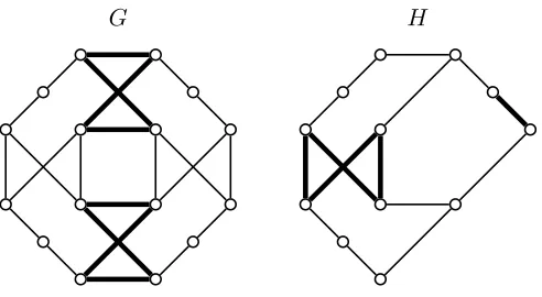
G H
Figure 2: Graph G that has a star cutset, but does not have an extreme connected non-path 2-join. G has a connected non-path 2-join represented with bold lines, and all connected non-path 2-joins are equivalent to this one. Both of the blocks of decomposition are isomorphic to graphH, and H has a connected non-path 2-join whose edges are represented with bold lines.
proof —If|A1|= 1 then by Lemma 4.1, (X1\A1, X2∪A1) is a connected
non-path 2-join of G, contradicting the assumption that (X1, X2) is mini-mally sided connected non-path 2-join ofG. So|A1| ≥2, and by symmetry |B1| ≥ 2. By Lemma 3.2 (iii), all vertices of A2 ∪B2 have degree at least
3. 2
Recall that aflat pathof a graphGis any path ofGof length at least 2, whose interior vertices all have degree 2 in G, and whose ends have no common neighbors outside the path.
Lemma 4.3 Let G∈ Cno sc and let (X1, X2, A1, B1, A2, B2) be a split of a minimally sided connected non-path 2-join of G. Let X1 be a minimal side, and let P be a flat path of G. If P ∩X1 =6 ∅ and P ∩X2 6= ∅, then one of the following holds:
(i) For an endvertex u of P, P\u⊆X1 and u∈A2∪B2.
proof — Letuand vbe the endvertices of P. By Lemma 4.2, the interior
of P must lie in X1 and w.l.o.g. u∈A2. By Lemma 3.2 (iii), the neighbor
x of u along P has a neighbor in X1, so |A2| = 1. Hence if (i) does not hold thenv∈B2. Also, P is of length at least 3. So, the interior ofP is a connected componentC of G[X1]. IfG[X1\C] is not a path with one end inA1, one end inB1 and interior inC1 then (X1\C, X2∪C) is a connected non-path 2-join. Indeed, by Lemma 3.2 (i), X1\C meets A1 and B1, and since it is not a path, it has size at least 3, so (X1\C, X2∪C) is a non-path 2-join that is connected by Lemma 3.2 (ii). This contradicts (X1, X2) being minimally-sided. Therefore (ii) holds. 2
Lemma 4.4 Let (X1, X2, A1, B1, A2, B2) be a split of a minimally-sided connected non-path 2-join of a graph G, with X1 being a minimal side. As-sume thatG and all the blocks of decomposition of G w.r.t. (X1, X2) whose marker paths are of length at least 3, all belong toCno sc. Then (X1, X2) is an extreme 2-join andX1 is an extreme side.
proof — Suppose that the block of decomposition Gk1
1 , k1 ≥ 3, has a connected non-path 2-join with split (X′
1, X2′, A′1, B′1, A′2, B2′). For i = 1,2 let Ci′ = Xi′\(A′i∪Bi′). Let P2 = x0−x1− · · · −xk1, where x0 = a2 and xk1 =b2, be the marker path of G
k1 1 .
Case 1: For somei∈ {1,2}, P2 ⊆Xi′.
W.l.o.g.P2 ⊆X2′. Note that sinceNGk1 1
(P2\ {a2, b2})⊆ {a2, b2}we have
P2∩(A′2∪B′2)⊆ {a2, b2}. Note also that sincea2 and b2 have no common neighbor inGk1
1 we have |A′2∩ {a2, b2}| ≤1 and |B2′ ∩ {a2, b2}| ≤1. So by symmetry it suffices to consider the following subcases:
Case 1.1: P2⊆C2′
Since a2 is adjacent to all vertices of A1 and a2 has no neighbor in X1′ (sincea26∈A′2∪B2′) it follows thatA1⊆X2′. Similarly B1 ⊆X2′. But then (X′
1,(X2′\P2)∪X2) is a connected non-path 2-join ofG. SinceA1∪B1⊆X2′,
X′
1 (X1, contradicting our choice of (X1, X2).
Case 1.2: a2 ∈A′2 and P2\ {a2} ⊆C2′.
Sob2has no neighbor inX1′, and sinceb2 is adjacent to all vertices ofB1, it follows that B1 ⊆X2′. In particular, X1′ (X1. Since a2 ∈ A′2, P2 ⊆X2′ and NGk1
1
But then (X′
1,(X2′ \P2)∪X2, A′1, B1′,(A′2 \ {a2})∪A2, B2′) is a split of a connected non-path 2-join ofG, contradicting our choice of (X1, X2).
Case 1.3: a2 ∈A′2,b2 ∈B2′ andP2\ {a2, b2} ⊆C2′. Since (X′
1, X2′) is not a path 2-join, X2′ ∩X1 6= ∅, and hence X1′ (X1. Since a2 ∈A′2, P2 ⊆ X2′ and NGk1
1
(a2)\P2 = A1, it follows that A′1 ⊆A1 and (X′
1\A′1)∩A1 =∅. Similarly B1′ ⊆B1 and (X1′ \B1′)∩B1 = ∅. But then (X′
1,(X2′ \P2)∪X2, A′1, B1′,(A2′ \ {a2})∪A2,(B′2\ {b2})∪B2) is a split of a connected non-path 2-join ofG, contradicting our choice of (X1, X2).
Case 2: Fori= 1,2,P2∩Xi′ 6=∅.
We may assume w.l.o.g. that (X′
1, X2′) is a minimally-sided connected non-path 2-join ofGk1
1 , withX1′ being the minimal side. But then by Lemma 4.3 applied to (X′
1, X2′) and P2 it suffices up to symmetry to consider the following two cases:
Case 2.1: a2 ∈A′2 and P2\a2 ⊆X1′.
Since x1 is of degree 2 andx2 ∈X1′, it follows that |A′2|= 1. Note that
P2\{a2, x1} ⊆X1′\A′1. Sincea2 ∈A′2,A′1\{x1} ⊆A1andA1\A′1⊆X2′\A′2. Note that since (X′
1, X2′) is connected,A1\A′1 6=∅. Note thatP2∩B1′ ⊆ {b2}. First suppose that b2 ∈ C1′. Since b2 is adjacent to all vertices of B1,
B1 ⊆X1′. By Lemma 3.2, (v), no vertex ofB′2 has a neighbor in A′2, which implies B2′ ∩A1 = ∅. So, C2′ 6= ∅ and by Lemma 3.2 (vi), |X2′| ≥ 4. But then (X′
2\ {a2},(X1′ \P2)∪X2, A1\A′1, B2′, A2, B′1) is a split of a connected non-path 2-join of G, contradicting our choice of (X1, X2) (since clearly
X2′ \ {a2}(X1).
Hence b2 6∈ C1′ and b2 ∈ B1′. Then B2′ ⊆ B1 and B1 \B2′ ⊆ X1′. By Lemma 3.2, (v), no vertex of B′
2 has a neighbor in A′2, which impliesB2′ ∩
A1 = ∅. So (X2′ \ {a2},(X1′ \P2)∪X2, A1 \A′1, B2′, A2,(B1′ \ {b2})∪B2) is a split of a connected non-path 2-join of G, contradicting our choice of (X1, X2) (since clearlyX2′ \ {a2}(X1).
Case 2.2: a2 ∈A′2,b2 ∈B2′ andP2\ {a2, b2} ⊆X1′. Thenx1 ∈A′1,xk1−1∈B
′
1 andP\ {a2, b2, x1, xk1−1} ⊆C
′
1. Sincex1 and
xk1−1 are of degree 2 inG
k1
1 , it follows thatA′2 ={a2}andB2′ ={b2}. Since
N Gk1
1
(a2) = A1∪ {x1}, it follows that A′1\ {x1} ⊆ A1 and A1\A′1 ⊆X2′. SimilarlyB′
1\ {xk1−1} ⊆B1 andB1\B
′
1 ⊆X2′. Since (X1′, X2′) is connected,
A1\A′1 6=∅ and B1\B1′ 6=∅. Since a2 and b2 have no common neighbor in
Gk1
{a2, b2}| ≥3. But then ((X1′\P2)∪X2, X2′\{a2, b2}, A2, B2, A1\A′1, B1\B1′) is a split of a 2-join ofG. By Lemma 3.2 (ii) this 2-join is connected. Since Gk1
1 [X2′] and G[X2] are not paths, this 2-join is a non-path 2-join. But then sinceX′
2\ {a2, b2}(X1, our choice of (X1, X2) is contradicted. 2
WhenMis a collection of vertex-disjoint flat paths, a 2-join (X1, X2) is M-independent if for every pathP from M we have eitherV(P)⊆X1 or
V(P) ⊆X2. These special types of 2-joins will have a fundamental role to play when it comes to computing a largest stable set.
Lemma 4.5 Let (X1, X2, A1, B1, A2, B2) be a split of a minimally-sided connected non-path 2-join of a graph G, with X1 being a minimal side. As-sume thatG and all the blocks of decomposition of G w.r.t. (X1, X2) whose marker paths are of length at least 3, all belong to Cno sc. Let M be a set
of vertex-disjoint flat paths of length at least 3 of G. If there exists a path P ∈ M such that P∩A16=∅and P∩A2 6=∅, then let A′1 =A2, and other-wise let A′
1 = A1. If there exists a path P ∈ M such that P ∩B1 6= ∅ and P ∩ B2 6= ∅, then let B1′ = B2, and otherwise let B1′ = B1. Let
X′
1 =X1∪A′1∪B1′ and X2′ =V(G)\X1′. Then the following hold:
(i) (X′
1, X2′) is a connected non-path 2-join of G.
(ii) (X′
1, X2′) isM-independent.
(iii) (X′
1, X2′) is an extreme 2-join of G and X1′ is an extreme side of this 2-join.
proof —If there exists a pathP ∈ Msuch thatP∩A1 =6 ∅andP∩A2 6=∅,
then by Lemma 4.3, either for an endvertexuofP,P\u⊆X1 andu∈A2; or for endvertices uand v of P,u∈A2,v∈B2 and P \ {u, v} ⊆X1. Since the intermediate vertices of P are of degree 2, it follows that |A2|= 1, and so (i) holds by Lemma 4.1 (possibly applied twice).
Let (X′
1, X2′, A′1, B1′, A′2, B2′) be the split of (X1′, X2′), where A2 ∈ {A′
1, A′2} and B2 ∈ {B1′, B2′}. By Lemma 4.3, applied to (X1, X2), paths
P ∈ M are one of the following types:
Type 1: P ⊆X1
Type 2: P ⊆X2
Type 3: For an endvertexu ofP,u∈A2 andP \u⊆X1.
Type 5: For endverticesuand vofP,u∈A2,v∈B2 andP\ {u, v} ⊆X1.
Note that since M is a collection of vertex-disjoint paths, at most one path ofMis of type 3 (resp. type 4), and if there exists a type 3 (resp. type 4) path then for every type 2 path P,P ∩A2=∅(resp. P ∩B2=∅). Also there is at most one type 5 path in M, and if such a path exists there are no type 3 and 4 paths inM, and for every type 2 pathP ofM,P∩A2=∅ andP∩B2 =∅. So by the construction of (X1′, X2′) all type 1 (resp. type 2) paths w.r.t. (X1, X2) stay type 1 (resp. type 2) w.r.t. (X1′, X2′), and all type 3, 4 and 5 paths w.r.t. (X1, X2) become type 1 w.r.t. (X1′, X2′). Therefore (ii) holds.
Fork1, k2 ≥3, letG1k1 andGk22 be the blocks of decomposition ofGw.r.t. the 2-join (X1, X2). By Lemma 4.4,Gk11 has no connected non-path 2-join. LetP2be the marker path ofGk11. LetG
′k′ 1
1 be the block of decomposition of
Gwith respect to (X′
1, X2′). Notice that G ′k′
1
1 can be obtained fromG
k1 1 by subdividing an edge ofP2 (0, 1 or 2 times), and hence by our assumption,
G′k1′
1 ∈ Cno sc. Therefore by Lemma 4.4, G
′k′ 1
1 has no connected non-path
2-join and hence (iii) holds. 2
Lemma 4.6 There is an algorithm with the following specification:
Input: A connected graph Gand a set Mof vertex-disjoint flat paths of G of length at least 3.
Output: One of the following is returned.
(i) An extreme connected non-path 2-join of G (with an identified extreme side) that is M-independent.
(ii) G or a block of decomposition of G w.r.t. some 2-join whose marker path is of length at least 3, has a star cutset.
(iii) Ghas no connected non-path 2-join.
Running time: O(n3m)
G is identified as having a star cutset return (ii) and stop, and otherwise continue.
Note that at this point in the algorithm we know that G∈ Cno sc, and
hence by Lemma 3.2 (ii) any 2-join ofG is connected.
Run the O(n3m)-algorithm from Theorem 5.2 in [2] for G. This algo-rithm outputs a minimally sided non-path 2-join of an input graph with no star cutset, or certifies that the input graph has no non-path 2-join. If this stage of the algorithm does not find any non-path 2-join in G, then return (iii) and stop. Otherwise let (X1, X2, A1, B1, A2, B2) be the split of a minimally-sided connected non-path 2-join found, and w.l.o.g. assume that X1 is a minimal side.
Let G31 and G32 be the blocks of decomposition of G w.r.t. (X1, X2). Check whether G31 and G32 have a star cutset. If any one of them does, then return (ii) and stop. Otherwise, we continue and we note that since
G31, G32∈ Cno scclearly blocks of decomposition ofGw.r.t. (X1, X2)G
k1 1 and
Gk2
2 , for anyk1, k2 ≥3, also belong to Cno sc.
If there exists a path P ∈ M such that P ∩A1 6= ∅ and P ∩A2 6= ∅, then letA′
1=A2, and otherwise letA′1=A1. If there exists a pathP ∈ M such thatP ∩B1 6=∅ and P∩B2 6=∅, then letB1′ =B2, and otherwise let
B′
1 =B1. LetX1′ =X1∪A′1∪B1′ andX2′ =V(G)\X1′. Then by Lemma 4.5, (X′
1, X2′) is an extreme connected non-path 2-join (withX1′ being an extreme side) that isM-independent. We return this 2-join in (i) and stop.
Clearly this algorithm can be implemented to run in time O(n3m). 2
Note that later when we apply the above algorithm in our main algo-rithm, if the output is (ii), then by Lemma 3.7 we can conclude thatGdoes not belong toCBerge
no cutset or to C
ehf
no sc.
5
Keeping track of cliques
Here we show how to find a maximum clique in a graph using 2-joins. For the sake of induction we have to solve the weighted version of the problem. Through all the next sections, by graph we mean a graph with weights on the vertices. Weights are numbers fromK whereK means either the set
graph whose vertices have all weight 1. Here, ω(G) denotes the weight of a maximum weighted clique of G.
Let (X1, X2, A1, B1, A2, B2) be a split of a connected 2-join of G. We define for k ≥ 3 the clique-block Gk
2 of G with respect to (X1, X2). It is obtained from the block Gk
2 by giving weights to the vertices. Let P1 =
a1−x1−· · ·−xk−1−b1 be the marker path of Gk2. We assign the following weights to the vertices ofGk
2:
• for everyu∈X2,wGk
2(u) =wG(u); • wGk
2(a1) =ω(G[A1]); • wGk
2(b1) =ω(G[B1]); • wGk
2(x1) =ω(G[X1])−ω(G[A1]); • wGk
2(xi) = 0, fori= 2, . . . , k−1.
Lemma 5.1 ω(G) =ω(Gk
2).
proof — Let K be a maximum weighted clique of G. We show that the clique-block Gk
2 has a clique of weight wG(K), and hence ω(G) ≤ ω(Gk2). If K ⊆ X2 then K ⊆ V(Gk2). If K ⊆ X1 then {a1, x1} is a clique of Gk2 of weight wG(K). So assume that K ∩X1 =6 ∅ and K∩X2 6=∅. W.l.o.g.
K∩A1 6=∅andK∩A2 6=∅, and henceK⊆A1∪A2. But then (K\A1)∪{a1} is a clique ofGk
2 of weight wG(K). Therefore ω(G)≤ω(Gk2).
Now let K be a maximum weighted clique of Gk
2. We show thatG has a clique of weight wGk
2(K), and hence ω(G
k
2)≤ω(G). If K⊆X2 thenK is a clique of G. SupposeK∩P1 ={a1}, and letK′ be a clique of A1 whose weight isω(G[A1]). Then (K∩A2)∪K′ is a clique of Gof weightwGk
2(K). So we may assume that K = {a1, x1}. Then wGk
2(K) = ω(G[X1]), and G has a clique of the same weight. Therefore ω(Gk
2)≤ω(G). 2
6
Keeping track of stable sets
some computations are done on its blocks as defined in Section 3. So we need to enlarge slightly our blocks to encode information, and this causes some trouble. First, the extended blocks may fail to be in the class we are working on. This problem will be solved in Section 8 by building the decomposition tree in two steps. Also in a decomposition tree built with our unusual blocks, the leaves may fail to be basic graphs, so computing something in the leaves of the tree is a problem postponed to Section 7.
Throughout this section, G is a fixed graph with a weight function w on the vertices and (X1, X2, A1, B1, A2, B2) is a split of a 2-join of G. For
i= 1,2, Ci = Xi\(Ai∪Bi). For any graph H, α(H) denotes the weight
of a maximum weighted stable set of H. We define a = α(G[A1∪C1]),
b=α(G[B1∪C1]), c=α(G[C1]) andd=α(G[X1]).
Lemma 6.1 Let S be a stable set of Gof maximum weight. Then one and only one of the following holds:
(i) S∩A1 6=∅, S∩B1 =∅, S∩X1 is a maximum weighted stable set of
G[A1∪C1] and w(S∩X1) =a;
(ii) S∩A1 =∅, S∩B1 6=∅, S∩X1 is a maximum weighted stable set of
G[B1∪C1] and w(S∩X1) =b;
(iii) S∩A1 =∅, S∩B1 =∅, S∩X1 is a maximum weighted stable set of
G[C1]and w(S∩X1) =c;
(iv) S∩A1 6=∅, S∩B1 6=∅, S∩X1 is a maximum weighted stable set of
G[X1]and w(S∩X1) =d.
proof —Follows directly from the definition of a 2-join. 2
6.1 Stable sets overlapping 2-joins
We need kinds of blocks that preserve being in CBerge
. To define them we need several inequalities that tell more about how stable sets and 2-joins overlap.
Lemma 6.2 0≤c≤a, b≤d≤a+b.
proof — The inequalities 0≤c ≤a, b≤d are trivially true. Let D be a
maximum weighted stable set ofG[X1]. We have:
2
A 2-join with split (X1, X2, A1, B1, A2, B2) is said to beX1-even (resp.
X1-odd) if all paths from A1 to B1 with interior in C1 are of even length (resp. odd length). Note that from Lemma 3.1, ifGis inCparity
and (X1, X2) is connected, then (X1, X2) must be either X1-even or X1-odd.
Lemma 6.3 If (X1, X2) is an X1-even 2-join ofG, then a+b≤c+d.
proof — LetA be a stable set of G[A1∪C1] of weight a and B a stable
set of G[B1∪C1] of weight b. In the bipartite graphG[A∪B], we denote by YA (resp. YB) the set of those vertices of A∪B such that there exists
a path inG[A∪B] joining them to some vertex of A∩A1 (resp. B∩B1). Note that from the definition,A∩A1 ⊆YA,B∩B1 ⊆YBand no edges exist
between YA∪YB and (A∪B)\(YA∪YB). Also, YA and YB are disjoint
with no edges between them because else, there is some path in G[A∪B] from some vertex of A∩A1 to some vertex of B ∩B1. If such a path is minimal with respect to this property, its interior is inC1 and it is of odd length becauseG[A∪B] is bipartite. This contradicts the assumption that (X1, X2) isX1-even. Now we put:
• ZD = (A∩YA)∪(B∩YB)∪(A\(YA∪YB));
• ZC = (A∩YB)∪(B∩YA)∪(B\(YA∪YB)).
From all the definitions and properties above,ZD andZC are stable sets
andZD ⊆X1 and ZC ⊆C1. So,a+b=w(ZC) +w(ZD)≤c+d. 2
Lemma 6.4 If (X1, X2) is an X1-odd 2-join of G, then c+d≤a+b.
proof — Let D be a stable set of G[X1] of weight d and C a stable set
of G[C1] of weight c. In the bipartite graph G[C ∪D], we denote by YA
(resp. YB) the set of those vertices of C∪D such that there exists a path
in G[C∪D] joining them to some vertex of D∩A1 (resp. D∩B1). Note that from the definition, D∩A1 ⊆ YA, D∩B1 ⊆ YB and no edges exist
between YA∪YB and (C∪D)\(YA∪YB). Also, YA and YB are disjoint
• ZA= (D∩YA)∪(C∩YB)∪(C\(YA∪YB));
• ZB= (D∩YB)∪(C∩YA)∪(D\(YA∪YB).
From all the definitions and properties above, ZAandZB are stable sets
andZA⊆A1∪C1 andZB ⊆B1∪C1. So,c+d=w(ZA) +w(ZB)≤a+b.2
6.2 Even and odd blocks
We call flat claw of a weighted graph G any set {q1, q2, q3, q4} of vertices such that:
• the only edges between theqi’s are q1q2,q2q3 and q4q2;
• q1 and q3 have no common neighbor in V(G)\ {q2};
• q4 has degree 1 in G andq2 has degree 3 in G.
Lemma 6.5 LetGbe a graph, Q={q1, q2, q3, q4}a flat claw of GandS′ a maximum weighted stable set ofG. Then one and only one of the following holds:
(i) q1 ∈ S′, q3 ∈/ S′ and S′ ∩Q is a maximum weighted stable set of
G[{q1, q2, q4}];
(ii) q1 ∈/ S′, q3 ∈ S′ and S′ ∩Q is a maximum weighted stable set of
G[{q2, q3, q4}];
(iii) q1 ∈/ S′, q3 ∈/ S′ and S′ ∩Q is a maximum weighted stable set of
G[{q2, q4}];
(iv) q1 ∈ S′, q3 ∈ S′ and S′ ∩Q is a maximum weighted stable set of
G[{q1, q2, q3, q4}].
proof —Follows directly from the definitions. 2
We define now the even block G2 with respect to (X1, X2). We keep
X2 and replace X1 by a flat claw on q1, . . . , q4 where q1 is complete to A2 and q3 is complete to B2. We give the following weights: w(q1) = d−b,
Lemma 6.6 Ifa+b≤c+dand ifG2 is the even block ofG, thenα(G2) =
α(G).
proof — Let S be a stable set of maximum weight in G. Then S must
satisfy one of (i), (ii), (iii) or (iv) of Lemma 6.1. Respective to these cases one can construct a stable setS′ of G
2 that has the weight of S, by taking the union ofS∩X2 and one of {q1, q4},{q3, q4},{q2} or{q1, q3, q4}.
Conversely, ifS′ is a stable set ofG
2 of maximum weight then it satisfies one of (i), (ii), (iii) or (iv) of Lemma 6.5. Respective to these cases,w(S′∩Q)
isa,b,cord(by Lemma 6.2 and becausea+b≤c+d) and one can construct a maximum stable setS ofG by replacing S′∩Q by a maximum weighted
stable set ofG[A1∪C1],G[B1∪C1], G[C1] orG[X1]. 2
We callflat vaultof graphGany set{r1, r2, r3, r4, r5, r6}of vertices such that:
• the only edges between theri’s are such thatr3, r4, r5, r6, r3 is a 4-hole;
• N(r1) =N(r5)\ {r4, r6};
• N(r2) =N(r6)\ {r3, r5};
• r1 and r2 have no common neighbors;
• r3 and r4 have degree 2 in G.
Lemma 6.7 Let G be a graph, Q = {r1, r2, r3, r4, r5, r6} a flat vault of G andS′ a maximum weighted stable set of G. Then one and only one of the
following holds:
(i) S′∩ {r
1, r5} 6=∅, S′∩ {r2, r6}=∅ andS′∩Q is a maximum weighted stable set of G[{r1, r3, r4, r5}];
(ii) S′∩ {r1, r5}=∅, S′∩ {r2, r6} 6=∅ andS′∩Q is a maximum weighted stable set of G[{r2, r3, r4, r6}];
(iii) S′∩ {r
1, r5}=∅, S′∩ {r2, r6}=∅ andS′∩Q is a maximum weighted stable set of G[{r3, r4}];
(iv) S′∩ {r
proof —Follows directly from the definitions. 2
Let us now define theodd block G2 with respect to (X1, X2). We replace
X1 by a flat vault on r1, . . . , r6. Moreover r1, r5 are complete to A2 and
r2, r6 are complete to B2. We give the following weights: w(r1) = d−b,
w(r2) = d−a, w(r3) =w(r4) =c, w(r5) = w(r6) = a+b−c−d. Note that if we supposec+d≤a+b (which holds in particular if (X1, X2) is an
X1-odd connected 2-join by Lemma 6.4), all the weights are non-negative by Lemma 6.2.
Lemma 6.8 If c+d≤a+b and ifG2 is the odd block of G, then α(G2) =
α(G).
proof — Let S be a stable set of maximum weight in G. Then S must
satisfy one of (i), (ii), (iii) or (iv) of Lemma 6.1. So, respective to these cases, it is easy to construct a stable setS′ of G
2 that has the weight of S, by taking the union of S ∩X2 and one of {r1, r3, r5}, {r2, r4, r6}, {r3} or {r1, r2, r3, r5}.
Conversely, if S′ is a stable set of G
2 of maximum weight then it sat-isfies one of (i), (ii), (iii) or (iv) of Lemma 6.7. Respective to these cases, w(S′ ∩Q) is a, b, c or d (because c+d ≤a+b) and one can construct a maximum weighted stable setS of Gof the same weight as S′ by replacing
S′∩ {r
1, r2, r3, r4, r5, r6} by a maximum weighted stable set of G[A1∪C1],
G[B1∪C1],G[C1] or G[X1]. 2
Note that the following lemma fails forCehf
because the odd block con-tains an even hole.
Lemma 6.9 LetGbe a graph inCBerge
and(X1, X2) be a connected 2-join ofG. If(X1, X2)isX1-even then the even blockG2is inCBerge. If(X1, X2) isX1-odd then the odd block G2 is in CBerge.
proof — Suppose that G2 contains an odd hole H. If no edge of H has
both ends inV(G2)\X2, thenH ⊆X2∪(NG2(A2)\X2)∪(NG2(B2)\X2). We obtain an odd holeH′ ofGas follows. By Lemma 3.2 (iv), there exist
non-adjacent vertices a1 ∈A1, b1 ∈B1. IfH∩(NG2(A2)\X2) 6=∅, we replace the unique vertex inH∩(NG2(A2)\X2) bya1. We proceed similarly with H∩(NG2(B2)\X2) andb1. We obtain an odd holeH
′ ofG, a contradiction.
and interior in C2. Then an odd hole of G can be obtained by replacing
q1−q2−q3 (resp. r5−r6) by a path of even (resp. odd) length ofG fromA1 to B1 with interior inC1. This contradictsGbeing Berge.
Suppose that G2 contains an odd antihole H. Since an antihole on 5 vertices is in fact a hole, we may assume that H is on at least 7 vertices. So all vertices ofH have degree at least four. Hence, ifG2 is an even block thenH cannot go through q2, q4. So, up to the replacement of at most two vertices, H is an odd antihole of G, a contradiction. Now supposeG2 is an odd block. Because of the degrees, r3, r4 ∈/ H. In an antihole on at least 7 vertices, every pair of vertices has a common neighbor. A vertex of{r1, r5} has no common neighbor with a vertex of{r2, r6}. So, we may assume that
H∩ {r2, r6}=∅. We have NG2(r1) ⊆NG2(r5) so not both r1, r5 are in H. So, we may assume thatr5∈/ H. So, up to the replacement ofr1 by a vertex ofA1,H is an odd antihole ofG, a contradiction. 2
6.3 The gem block
We present here a block of decomposition that we do not use in the rest of the paper but that is interesting because it can be used in all situations (whereas some inequalities must be satisfied for even and odd blocks).
To build the gem-block G2 replace X1 by an induced path p−x−y−p′ plus a vertexzcomplete to this path. Vertex pis complete toA2 and vertex
p′ is complete toB
2. We give weights: w(p) =a,w(x) =a+b−d,w(y) =d,
w(p′) = 2d−a, w(z) = c+d. Note that all weights are non-negative by
Lemma 6.2. We omit the proof of the following Lemma since we do not use it.
Lemma 6.10 If G2 is the gem-block of G then α(G2) =α(G) +d.
The gem-block appears implicitly in the proof of the NP-completeness result in Section 10.
7
Extensions of basic classes
To build a decomposition tree that allows keeping track of maximum stable sets we use the even and odd blocks defined in Section 6. As a consequence, the leaves of our decomposition tree may fail to be basic, but are what we call extensions of basic graphs. Let us define this.
Let P =p1−· · ·−pk, k≥ 4, be a flat path of a graphG. Extending P