Optimization methods for the real-time inverse problem posed by modelling of liquefied natural gas storage

White Rose Research Online

[email protected]

Universities of Leeds, Sheffield and York

http://eprints.whiterose.ac.uk/

This is an author produced version of a paper published in

Chemical

Engineering Journal

.

White Rose Research Online URL for this paper:

Published paper

Deshpande, K.B., Zimmerman, W.B., Tennant, M.T., Webster, M.B.,

Lukaszewski, M.W. (2011)

Optimization methods for the real-time inverse

problem posed by modelling of liquefied natural gas storage

, Chemical

Engineering Journal, 170 (1), pp. 44-52

Page 1 _of 29

Optimization methods for the real–time inverse problem

posed by modelling of liquefied natural gas storage

Kiran B. Deshpande, William B. Zimmermana, Malcolm T. Tennantb,

Marcus B. Websterb and Michal W. Lukaszewskia,b

a

Department of Chemical and Biological Engineering, University of Sheffield, Mappin Street, Sheffield, S1 3JD, England.

b

MHT Technology Ltd., Harelands Courtyard offices, Moor Road, Melsonby, Richmond, North Yorkshire, DL10 5NY, England.

Abstract

If two liquefied natural gases (LNG) obtained from two different sources are

inappropriately fed into a storage tank, lighter LNG may lie over heavier LNG forming a stratification, which could eventually lead to a rollover. Few models available in the literature predict time to rollover in LNG storage tanks. These are semi-empirical in

nature as they are based upon empirical correlations to estimate heat and mass transfer coefficients across the stratified layers. We present a lumped parameter

model in order to predict time to rollover and to investigate its sensitivity to variation of heat and mass transfer coefficients. The novelty of the present work is its ability to

estimate heat and mass transfer coefficients from the real time data using an inverse methodology. We assimilate the real time LNG level–temperature–density (LTD) data

from LNG storage tank in order to estimate heat and mass transfer coefficients from the densities of the stratified layers. The optimized heat and mass transfer

coefficients are then used to predict time to rollover. We present a sequence of LTD profiles obtained from real time LNG terminal and which are leading to rollover in one case study (Section 4.1). The time to rollover predicted using this inverse

methodology is compared with the LTD profiles obtained from real LNG tank and also with time to rollover obtained using empirical correlations. Heat transfer coefficients

estimated using empirical correlations are found to be over-estimated for some case studies, which under predict time to rollover. For the real time case study, time to

Page 2 _of 29

1. Introduction

In today’s globalised market of the liquefied natural gas (LNG) industry, LNG bought from different sources has potentially different density due to different composition.

Although composition of LNG varies depending on its source, it is mainly comprised of methane, ethane, propane, butane and traces of nitrogen. When fresh LNG is fed into a tank, the composition and temperature of LNG already in the tank could be

different to the fresh LNG. This could result in stratification of the tank; commonly known as fill induced stratification, due to inappropriate filling of the tank with LNG of

different densities. This stratification could eventually lead to a phenomenon called rollover. If the stratification is significant, then the LNG in the lower layer of the

stratified tank can become superheated, as it receives heat from the sidewalls and the bottom of the tank, which cannot escape to the vapour phase due to a cover

formed by LNG in the upper layer. The schematic of an LNG storage tank and the processes involved is shown in Fig. 1. The densities of the two layers eventually

equalize due to heat and mass transfer between the stratified layers and boil-off from the top surface. The hotter LNG in the lower layer comes to the top releasing all the heat it contained during incubation. This phenomenon is called “rollover” and could

be potentially dangerous due to the possibility of a higher boil-off rate at the time of rollover increasing the vapour pressure in the tank. The severity of the rollover event

depends upon the state of stratification and temperature gradient between the stratified layers and is addressed in detail in this article.

Natural gas is normally stored in a liquefied state, as the natural gas is compressed

by as much as 600 times when liquefied and is stored at just above atmospheric pressure and at a temperature of around –160 °C. As liquefied natural gas (LNG) is

stored at such a low temperature, there is a significant heat leakage from the surroundings into the tank varying the temperature inside the tank. The composition

of LNG in the stratified layers may also vary due to evaporation (boil–off) at the surface and mass transfer between the stratified layers. This requires continuous

monitoring of the tank particularly for temperature and density. In this article, we describe a lumped parameter model, which is developed to predict the behaviour of LNG inside a storage tank leading to rollover from the fundamental principles of

Page 3 _of 29 In the literature, there are only a couple of well-documented experimental evidences of LNG stratification resulting into rollover [1,2]. However, there are quite a few

theoretical models available in the literature (Chaterjee and Geist [3,4]; Germeles [5]; Heestand et al. [6]; and Bates and Morrison [7]). Chaterjee and Geist [3] considered

only two chemical species: methane and non-volatile heavy hydrocarbon and the rollover criterion considered in their approach was equal temperature and

composition of the stratified layers. Germeles [5] reported that equal density should be the rollover criterion instead of equal temperature and composition, as there

would be no change in vapour pressure and boil-off rate, if the latter is considered. Heestand et al. [6] considered the five most common constituents of LNG namely

methane, ethane, propane, n butane and nitrogen. Heestand et al. [6] argued about the use of thermohaline heat and mass correlations of Turner [8] in the previous models, as those correlations were provided for salt-water experiments and claimed

that these correlations significantly under-estimate mass transfer between the

stratified layers. Instead, Heestand et al. [6] assumed fully turbulent conditions inside the LNG storage tank and used the correlation of Globe and Dropkin [9] for heat transfer between two horizontal plates heated from the bottom. Heestand et al. [6]

also reported that rollover predictions are acutely sensitive to proportionality constant in empirical correlation and +20% change in this constant can lead to –15% change

in predicted time to rollover.

Chaterjee and Geist [3] and Bates and Morrison [7] assumed that LNG in the upper of the stratified layers is in thermodynamic equilibrium with the evolving vapours and

hence, temperature of the upper layer was assumed to be constant. They justified the above assumption by reporting that under normal operating conditions, all the

heat leakage into the tank is converted directly into the latent heat of vapourisation. Heestand et al. [6] assumed a thin film at the top surface of LNG, which is in thermodynamic equilibrium with the evolving vapours instead of the entire content in

the upper layer. The same approach (Heestand et al. [6]) is used in the present work, as it explains the peak in boil-off rate at the time of rollover.

In the present work, we consider the two stratified layers and temperature and

composition of LNG are averaged over the respective layers. The change in temperature and composition of LNG in each layer, due to heat leakage into the tank,

heat and mass transfer between the stratified layers, and boil-off from the top surface, is calculated by applying material and energy balance equations. LNG at the

Page 4 _of 29 vapours. The heat and mass transfer rates between the stratified layers is conventionally calculated using heat and mass transfer coefficients, which are

obtained from the empirical correlation (Globe and Dropkin [9]). The boil-off rate attains a peak at the time of rollover, as there is still a temperature gradient between

the stratified layers just before rollover and hence, relatively hotter LNG comes to the surface increasing the evaporation rate.

All the above models that we briefly discussed in this section are semi-empirical as

they use empirical correlations to evaluate heat transfer coefficients (HTC) and mass transfer coefficients (MTC). It is reported that rollover prediction is sensitive to heat

transfer between the stratified layers (Heestand et al. [6]) and hence, it is very important to estimate heat and mass transfer coefficients accurately. The novelty of the present work comes from its ability to estimate heat and mass transfer

coefficients from the real time data of the stratified tank. In this work, we propose a

methodology called “inverse method” where heat and mass transfer coefficients are estimated from the real time LTD (level–temperature–density) gauge data.

This article is organized as follows: the lumped parameter model is first discussed in detail describing material and energy balance equations and vapour liquid equilibrium

considered at the top surface of LNG. Rollover predictions for the two well documented incidents, La Spezia, 1971 and Partington, 1993, using empirical

correlation are presented in the model predictions section followed by the sensitivity analysis of rollover prediction based upon empirical heat and mass transfer

coefficients. The inverse methodology is then discussed in order to estimate heat and mass transfer coefficients from the real time LTD data, which are later used to predict

time to rollover and is followed by the conclusion section.

2.

Lumped parameter model

The lumped parameter model can be applied to both top filled and bottom filled

operations by feeding in appropriate molar flow rates, as discussed in the governing equations section. Here, we first consider the tank, which is filled from the bottom (La

Spezia, 1971) and then the tank, which is already filled and stratified (Partington, 1993). LNG of different compositions has different densities and hence, it tends to be

Page 5 _of 29 thin film region at the top of upper layer, which is in thermodynamic equilibrium with evolving vapours. As LNG is stored below –160 °C, there is a continuous heat

leakage from the bottom and sidewalls of the tanks. The heat leakage from the bottom is represented as qb, heat leakage from the top is represented as qt, where as that in the lower layer, upper layer and vapour space from the side walls are represented by qUL, qLL and qV, respectively.

Fig. 1. Schematic of LNG storage tank

2.1 Governing equations:

The change in composition and temperature of LNG in each layer can be estimated

by applying material and energy balance to the individual layers. The model gives flexibility of choosing any number of species up to a maximum of 10. It is assumed

that there is no accumulation of mass in the film layer and LNG in the film region is in thermodynamic equilibrium with evolving vapours. Representative material and

Page 6 _of 29 2.1.1 Material balance:

Lower layer: (1)

Upper layer: (2)

In the above equation (Eq. 1) for lower layer, the rate of change in composition of

species i is evaluated by considering molar flow rate of species i from cargo to lower layer of the tank (in case of bottom filling), and mass transfer flux between lower and

upper layers. Material balance for upper layer is written in a similar fashion as for lower layer (Eq. 1) with the only additional term for molar flow rate of evaporation

from upper layer to the vapour space, which is also called boil-off. Molar evaporation rate from the top surface is,

(

)

(

)

(

)

& (3)

fQ is the fraction of total heat transmitted to the vapour space, which is returned to

liquid and is assumed to be 95% [6].

t V VS

Q=q +q

π δ

Enthalpy of liquid and vapour phase is correlated in terms of temperature from which

specific heat can be estimated. Correlations for enthalpy of liquid and vapour phase are obtained from The Natural Gas Industry textbook by Medici [10].

Rayleigh recirculation liquid flow rate between upper layer and the film,M&R, can be evaluated as, 3 1 , 3276 . 0 _      _∆ = _R R u L R g C M

ρ

υα

ρ

κ

Concentration of LNG is calculated from average density and average molecular

weight of LNG in the respective layers. Density of LNG is calculated using Klosek-McKinley correlation (Klosek and Klosek-McKinley 1968; Boyle 1972) which incorporates the

dependence upon temperature and composition of LNG and is represented as,

(6)

[

]

d

C x i M A x i x i x i

dt

δ

κ

•

= ⋅ − ⋅ −

[

]

d

C x i M A x i M y i x i x i

dt

δ

κ

• • = ⋅ − − ⋅ − ( ) ( ) ( , ) i i

i i m

i

m K methane K

x MW x V V

V f T V C x

C f T MW

Page 7 _of 29 The molar volume, Vi, depends upon temperature and this dependence is obtained

from molar volume tabulation for various species reported in Boyle [19]. Vm is the

molar volume for methane. The correction factor, CK, is a function of temperature and

molecular weight of the mixture and this functionality is also obtained from the

tabulation reported in Boyle [19].

Composition of species in the vapourizing film can be estimated by applying Raoult’s law and can be written as,

(7)

The saturation pressure can be obtained from Antoine equation, which is discussed later in Section 2.1.4.

In addition to lower layer and upper layer, material balance is also applied to the film

region, which is assumed to be in equilibrium with evolving vapours, to estimate the composition of LNG in the film.

( )

(

)

( )

( )

& _{+ −}

= (8)

The composition of LNG in the film is later used to estimate average molecular weight and enthalpy of LNG in the film region.

2.1.2 Energy balance

Lower layer:

(

)

[

]

(

)

(

)

l LL b l l L l l l L l

l

h

T

T

A

D

q

q

T

T

C

A

M

T

T

C

C

dt

d

−

−

+

+

−

=

−

π

δ

δ

&

Upper layer:

(

)

[

]

Q V V u u L u u u L u

u h T T

A D q A Q f H M T T C A M T T C C dt d − − +       + − − = −

⋅

_π

_δ

δ

(10)

The rate of change in heat content of the lower layer is calculated by considering the

rate of heat coming in from cargo to lower layer (in case of bottom filling), the rate of heat transferred from the bottom of the tank, the rate of heat transferred from the side

walls of the tank and the rate of heat transfer between lower and upper layers.

( ) ( )

sat i

u P

y i x i P

Page 8 _of 29 Similarly, the rate of change in heat content of upper layer can be calculated by incorporating rate of heat transfer from cargo to upper layer (in case of top filling),

fraction of total heat returned from vapour space to upper layer, rate of heat transfer from side walls and the rate of heat transfer between lower and upper layers. Specific

heat of LNG in lower and upper layer is calculated from enthalpy correlations taken from Medici [10].

Heat and mass transfer rates between the stratified layers are traditionally estimated

from the empirical correlations. The empirical correlation of Globe and Dropkin [9] is more appropriate to estimate heat transfer coefficients in this work, as it was

proposed for heat transfer between the two horizontal plates heated from below and can be expressed as,

3 1 2 3

0597

.

0

_











∆

=

ρ

υ

ρ

κ

L

g

L

h

The proportionality constant in the above correlation is quite significant, as Heestand

et al. [6] reported that the time to rollover is sensitive to this parameter. We will address the issue of sensitivity later in this article.

Assuming turbulent conditions inside the tank, mass transfer coefficient can be

obtained from:

(12)

The temperature of LNG in the film region is estimated from the saturation pressure,

in order to match vapour pressure to the tank pressure.

2.1.3 Stratification forecast:

In the lumped parameter model, overall mass balance equations can be incorporated along with material balance and energy balance equations, in order to evaluate layer

thickness of each layer. The evolution of an individual layer is strictly based on initial stratification and operating conditions.

(13) (14) (15) 1 [ / ( ( ) ( ))] / N l

l l u l l

i d

M A x i x i MW

dt

δ

κ

ρ

∑

l u V u u

i d

x i x i M MW dt

δ

κ

ρ

=

= ⋅

∑

VS

L

δ

=

−

δ

−

δ

Page 9 _of 29 The evolution of lower layer is estimated from molar flow rate from cargo to lower layer (in case of bottom filling) and mass transfer rate between two layers, whereas

for upper layer there is an additional term of mass lost due to boil–off. The thickness of vapour space is estimated from total height of the tank and lower and upper layer

thickness.

2.1.4 Preferential boil–off

LNG is mainly comprised of methane, ethane, propane, and butane with the traces of

nitrogen. The boiling points of these species vary considerably with nitrogen boiling preferentially followed by lighter hydrocarbons. The lumped parameter model

incorporates preferential boil-off of more volatile species using vapour liquid equilibrium. The saturation pressure of individual species is obtained from Antoine

equation, which is represented as,

10

A A

A

log

P

A

B

T

C

=

−

+

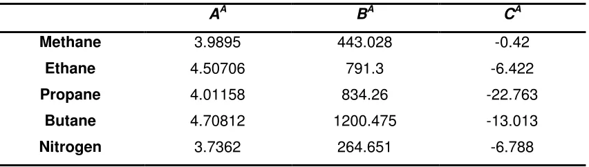
where, Psat is saturation pressure in bar a, T is temperature in K, and AA, BA and CA are Antoine constants, which can be obtained from the literature. The Antoine constants for the main constituents of LNG are tabulated in Table 1.

Table 1. Antoine constants for major constituent of LNG

AA BA CA

Methane 3.9895 443.028 -0.42

Ethane 4.50706 791.3 -6.422

Propane 4.01158 834.26 -22.763

Butane 4.70812 1200.475 -13.013

Nitrogen 3.7362 264.651 -6.788

The Antoine equation estimates the highest saturation pressure for nitrogen followed

Page 10 _of 29

3.

The model results:

In this section, the lumped parameter model is applied to the two case studies namely La-Spezia, Italy [1] and Partington, UK [2], where rollover incidents occurred

and which are well documented in the literature. The model predictions are subjected to various operating parameters and initial conditions for temperature, composition

and level of stratified layers of the storage tank. Various heat leakage rates from bottom, top and sidewalls to lower and upper layer and physical properties of LNG

such as thermal conductivity, thermal diffusivity and kinematic viscosity also contribute towards predicting time to rollover.

3.1 La Spezia case study:

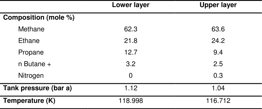
Sarsten [1] reported La Spezia rollover incident elaborating the filling operation of tank, composition of LNG in cargo and heel, various operating conditions inside the tank such as tank pressure. The composition of LNG in lower and upper layer, used

in this work is summarised in following table, where hydrocarbon chains up to n butane are considered.

Table 2. Various operating parameters for the stratified layers inside the tank that are used in

this work to predict time to rollover are tabulated here.

Lower layer Upper layer

Composition (mole %)

Methane

Ethane Propane

n Butane + Nitrogen

62.3

21.8 12.7

3.2 0

63.6

24.2 9.4

2.5 0.3

Tank pressure (bar a) 1.12 1.04

Temperature (K) 118.998 116.712

It should be noted that temperature of the stratified layers of LNG inside the tank are not reported by Sartsen [1] and hence, temperature of the stratified layers, as

Page 11 _of 29 inside the tank and composition of LNG, in order to match the vapour pressure of LNG and the tank pressure.

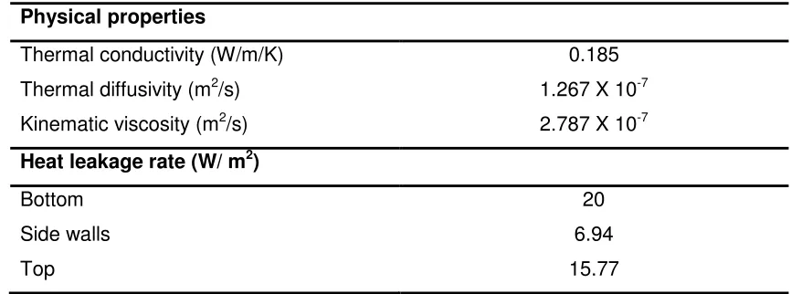
Various physical properties and heat leakage rates are tabulated in Table 3.

Table 3: Physical properties and heat leakage rate considered for La Spezia case study

Physical properties

Thermal conductivity (W/m/K) 0.185

Thermal diffusivity (m2/s) 1.267 X 10-7 Kinematic viscosity (m2/s) 2.787 X 10-7

Heat leakage rate (W/ m2)

Bottom 20

Side walls 6.94

Top 15.77

The tank is bottom filled at the rate of 0.72 m3/s and filling time was about 13 hrs. Tank diameter is 49 m and tank height is 26.77 m. The initial depths of lower layer

and upper layer, before filling started, were 1.3716 m and 5.029 m, respectively. The tank is kept at the constant atmospheric pressure of 1.01325 bar a. Based upon the

above operating parameters and physical properties, the model can be executed for the specified time and the evolution of various parameters can be predicted, as

discussed below.

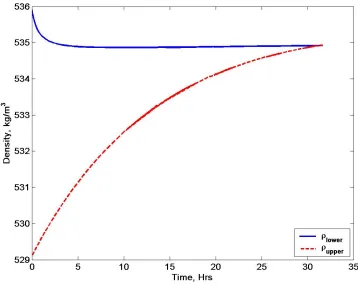
3.1.1 Evolution of density

The density profiles of lower layer and upper layer, predicted using the lumped parameter model are shown in Fig 2. Density of the lower layer, as represented by

solid line, decreases with time, whereas that of upper layer, as represented by dashed line, increases with time due to heat and mass transfer between the stratified

layers and boil–off from the upper layer. Densities of the stratified layers eventually attain a uniform value. Density equalization is the criterion for prediction of rollover

using the lumped parameter model. It can be seen that rollover occurs at about 31 h and 37 minutes, which is in a good agreement with the reported value of Sartsten [1]

Page 12 _of 29 Fig. 2. The density profile of lower and upper layer of LNG obtained using the lumped

parameter model is plotted against time.

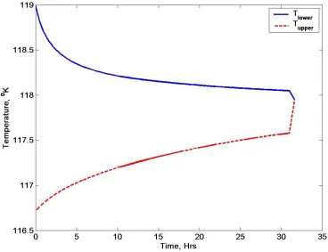
3.1.2 Evolution of temperature

The temperature profile of LNG in the lower and upper layers obtained using the

lumped parameter model is shown in Fig. 3. It can be seen that temperature of lower layer decreases with time and that of upper layer increases with time. Although, the

bottom layer is getting significant energy through heat leakage from the bottom and side walls, there is considerable heat transfer between the stratified layers. It can

also be seen that there exists a temperature gradient between the two layers, even

just before rollover, which contributes to the higher boil–off rate at the time of rollover.

Thus, the magnitude of severity of rollover due to higher boil–off rate is subjected to

the temperature gradient, just before the rollover. After rollover, the two layers mix

Page 13 _of 29 Fig. 3. Temperature profile of lower and upper layer of LNG obtained using the lumped

parameter model is plotted against time.

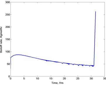
3.1.3 Evolution of boil–off rate

Boil-off rate predicted using the lumped parameter model is plotted against time, as

shown in Fig. 4. It can be seen that boil–off rate peaks at the time of rollover. A peak

in boil-off rate is due to the temperature gradient at the time of density equalisation. The temperature of LNG in the upper layer increases by almost 0.5 K after the

rollover event increasing boil-off rate. The present model predicts the boil-off rate until the occurrence of rollover correctly, which is about 40 kgmol/hr and is in very

good agreement with 1000 kg/hr (about 43 kgmol/hr) as reported for the La Spezia

incident [1]. However, it should be noted that the exact extent of boil–off rate at the

time of rollover can not be predicted due to instantaneous nature of the rollover

event, as reported by Heestand et al. [6]. For the La Spezia incident, Sarsten [1] reported that 300,000 lbs of LNG vapour lost during 1.25 hrs of rollover event, which

is equivalent of 100,000 kg/hr. Thus, boil–off rate was about 100 times higher than

that just before rollover. We can correctly predict the time to rollover, but the extent of

Page 14 _of 29 Fig. 4. Boil of rate obtained using the lumped parameter model is plotted against time

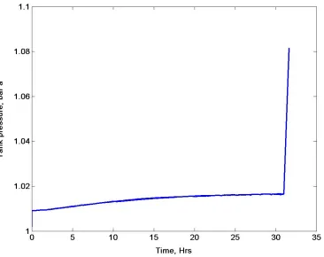
3.1.4 Evolution of tank pressure

In the present work, rollover predictions are based upon constant tank pressure of 1.01325 bar a. Composition and temperature of LNG at the top surface varies

continuously due to boil–off rate and heat and mass transfer between the stratified

layers. The change in vapour pressure due to above dynamic conditions is plotted in Fig. 5. It can be seen that vapour pressure increases slightly due to the increase in

boil-off rate until just before rollover. At the time of rollover, boil-off rate increases rapidly due to which tank pressure also increases significantly. The change in the saturation pressure due to boil-off can be estimated by the correlation reported by

[12], which can be represented as,

boiloff rate=0.0082× ∆Ps4 / 3 (17) Boiloff rate is in lbs/hr/ft2 and ∆Psis supersaturation pressure in inches of water. At the time of rollover, tank pressure estimated using the above correlation matches

Page 15 _of 29 Fig. 5. The change in tank pressure obtained using the lumped parameter model is plotted

against time

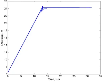
3.1.5 Evolution of LNG level

The tank filling can be captured using the lumped parameter model. In Fig. 6, the evolution of the total height of LNG in the tank due to bottom filling of the tank is

Page 16 _of 29 Fig. 6. The evolution of LNG level obtained using the lumped parameter model is plotted

against time

3.2

Partington case study:

In 1993, a rollover occurred in a British Gas LNG storage tank at the Partington site.

Baker and Creed [2] provided a detailed account of various storage conditions inside the tank such as LNG level of the stratified layers, density, composition of LNG in stratified layers and heat leakage rate into the tank. Various parameters used in this

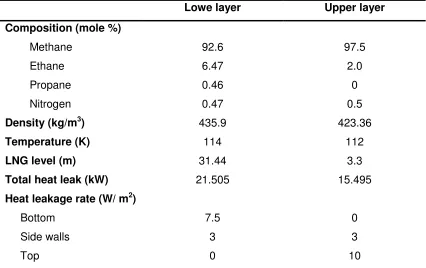
case study are summarised in Table 4.

The tank is kept at the constant pressure of 1.08 bar a. It should be noted that temperatures of the stratified layers of LNG inside the tank are not reported in Baker

and Creed [2] and hence, temperatures of the stratified layers, as reported in Table 4, are estimated from density and composition of LNG in the stratified layers.

Physical properties of LNG as reported for the La Spezia case study are used here. Heat leakage rates are calculated from the total heat leak into the stratified layers, as

Page 17 _of 29 Table 4. Various operating parameters for the stratified layers inside the tank that are used for

Partington case study in order to predict time to rollover are tabulated here.

Lowe layer Upper layer

Composition (mole %)

Methane

Ethane Propane

Nitrogen

92.6

6.47 0.46

0.47

97.5

2.0 0

0.5

Density (kg/m3) 435.9 423.36

Temperature (K) 114 112

LNG level (m) 31.44 3.3

Total heat leak (kW) 21.505 15.495

Heat leakage rate (W/ m2)

Bottom

Side walls Top

7.5

3 0

0

3 10

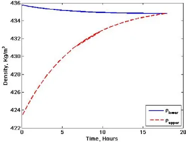
3.2.1 Evolution of density

Density profiles of LNG in the stratified layers, predicted using the lumped parameter

model for operating parameters reported in Table 4, are shown in Fig. 7. It can be seen that density of the lower layer decreases slightly, whereas that of upper layer

Page 18 _of 29 Fig. 7. The density profile of lower and upper layer of LNG obtained using the lumped

parameter model is plotted against time for the Partington case study.

3.2.2 Evolution of boil–off rate

The boil–off rate predicted for the Partington case study is shown in Fig. 8. It should

be noted that although the boil–off rate follows the similar trend as for the La Spezia case study, the major issue in the predictions for the Partington case study is that the

time to rollover is severely under predicted. Baker and Creed [2] reported that rollover occurred after 68 days, whereas the predicted time to rollover is 18 h using

the empirical correlation. This under-prediction could be attributed to the higher heat and mass transfer rates between the stratified layers, which would enhance the mixing between the layers predicting earlier time to rollover. This case study

Page 19 _of 29 Fig. 8. The boil–off rate obtained using the lumped parameter model is plotted against time for the Partington case study.

3.3 Sensitivity of empirical correlations:

The predictions made for time to rollover using the lumped parameter model are sensitive to heat and mass transfer rate between the stratified layers and hence, are

also subjected to empirical constant used while estimating heat transfer coefficient. Heestand et al. [6] also reported that +20% change in empirical constant leads to –

15% change in the predicted time to rollover. We performed computational runs by using various empirical constants for the La Spezia case study and the predicted

time to rollover are reported in Table 5.

It can be seen (Table 5) that the predictions of time to rollover are very sensitive to

empirical constants and the predictions can vary form 27 h to about 40 h depending upon the empirical constant used for heat transfer coefficient estimation.

In addition to uncertainty over which empirical constant should be used or what

Page 20 _of 29 assuming turbulent conditions within the stratified layers. The correct estimation of heat and mass transfer coefficients is the necessity for an accurate prediction of time

to rollover. Hence, we propose a unique methodology, wherein heat and mass transfer coefficients can be estimated from the real time level–temperature–density

data, and is discussed in the next section.

Table 5: Predicted time to rollover using various empirical constant.

Correlation used Time to rollover

Nu = 0.0493 (Gr)1/3

([18], without Prandlt number)

38 h 46 min

Nu = 0.064 (Gr)1/3

([19], with Prandlt number)

31 h 37 min

Nu = 0.0597 (Gr)1/3

([9], without Prandlt number)

33 h 3 min

Nu = 0.077 (Gr)1/3

([9], with Prandlt number)

26 h 30 min

Nu = 0.05513 (Gr)1/3

([6], with Prandlt number)

35 h 24 min

4.

Inverse methodology via optimization

In the lumped parameter model as discussed in Section 3, heat transfer coefficient

was obtained from an empirical correlation. The mass transfer coefficient was then calculated from the heat transfer coefficient assuming turbulent conditions inside the

individual layers. The time to rollover is sensitive to heat and mass transfer coefficients between the stratified layers and hence, an accurate prediction of heat

and mass transfer coefficients is essential for accurate rollover prediction. Hence, we developed a novel technique where heat and mass transfer coefficients can be

estimated using the inverse methodology from the real time LTD profiles. Deshpande and Zimmerman [17] applied the inverse methodology to estimate mass transfer coefficients of the premixed reactants in order to study transport limited

characteristics of instantaneous reaction with asymmetric transport rates. Other

Page 21 _of 29 filter (Baratti et al., 1995) and extended Luenberger observer (Quintero-Marmol et al., 1991), typically for online control systems.

The governing equations of the lumped parameter model are first solved for the initial guess of heat and mass transfer coefficients to estimate the change in density over a

specific time. LTD profiles taken over the same time provide the actual change in density in the tank. The error is calculated from density obtained for the guessed

values and the actual density obtained from LTD gauge and is represented as,

2 , , , 2 , , ,

















₋

+

















₋

=

error

ρ

ρ

ρ

ρ

ρ

ρ

Where

ρ

ρ

of the lower layer,

ρ

ρ

the measured density of the upper layer.

Estimated densities are calculated from composition and temperature of the stratified layers using Klosek–McKinley equation (Eq. 6) while measured densities are those obtained from LTD gauge. In the inverse method, the lumped parameter model is

iteratively solved by varying heat and mass transfer coefficients until the estimated

error reaches the prescribed tolerance. Thus, heat and mass transfer coefficients are estimated so that the calculated density change matches with the actual density change (obtained from LTD profiles). The above procedure is schematically shown

in Fig. 9.

The termination criterion used in this optimization procedure is the tolerance of

0.1 %. Once the error estimated during optimization reaches this tolerance, optimization is terminated fetching heat and mass transfer coefficients corresponding

to that error. The guessed heat and mass transfer coefficients can be varied to check uniqueness of the estimated heat and mass transfer coefficients. We performed

various computational runs by varying initial heat and mass transfer coefficients by the orders of magnitude and the predicted heat and mass transfer coefficients are

found to be of the same order of magnitude. The predicted heat and mass transfer coefficients are not reported in this article due to their commercial sensitivity.

We apply the above methodology for the two case studies with data obtained from

Page 22 _of 29 Fig. 9. Schematic of the procedure used to infer HTC and MTC from the real time LTD data

Page 23 _of 29

4.1 Case study 1

In this case study, we present the level–temperature–density profiles, which capture the occurrence of rollover event. Four LTD data sets are reported in Table 6. LTD

profile 2 and 3 are taken after 26 h and 60 h, respectively, after taking the profile 1. LTD profile 4 represents the occurrence of rollover event as densities of the stratified

layers equalize after 258 h, after talking profile 1. This case study provides vital information in order to predict the correctness of prediction of time to rollover.

Table 6. LTD data for the four profiles used in order to estimate heat and mass transfer

coefficients and to predict time to rollover is presented here.

LTD profile 1 LTD profile 2 LTD profile 3 LTD profile 4

Lower layer

Level, m

Temperature, K Density, kg/m3

21 112.6 432.6

19 112.68

432.5

17 112.73

432.4

24 112.23

432.6

Upper layer

Level, m

Temperature, K

Density, kg/m3

3 111.93

429.2

5 112.09

430.6

7 112.19

431.4

0 112.25

432.6

The inverse methodology, as discussed in the schematic as shown in Fig. 9, is applied to the two data sets in pairs (profile –profile 2 and profile 1–profile 3) in order

to estimate heat and mass transfer coefficients from the change in density of the stratified layers. The same composition, heat leakage rate and physical properties, as mentioned in Table 4 for the Partington case study, are used here. A pair of

profiles is used to estimate heat and mass transfer coefficients, which are then used to predict time to rollover based upon the latest profile.

For the first data set pair (profile 1–profile 2), the predicted time to rollover is 7 days

and 14 h and for the second data set pair, it is 10 days and 13 h. The real time profiles obtained from LNG storage tank farm indicated that rollover occurred after

Page 24 _of 29 methodology are close to the real time LTD profiles and certainly a lot better than the predictions based upon empirical correlations where the predicted time to rollover is

1day 13 h and 1 day and 20 h for the first and second data set pair, respectively. The rollover prediction obtained using the inverse method is substantially better than

those using the empirical correlation.

4.2 Case study 2

In the second case study, the three LTD profiles tabulated in Table 7 are considered.

LTD profile 2 was taken 32 h after the profile 1, whereas profile 3 was taken 92 h after the profile 1.

Table 7. LTD data for the three profiles used in order to estimate heat and mass transfer

coefficients is presented here.

LTD Profile 1 LTD Profile 2 LTD Profile 3

Lower layer

Level, m

Temperature, K Density, kg/m3

24

112.43 433.3

23

112.47 433.3

21

112.54 433.1

Upper layer

Level, m Temperature, K

Density, kg/m3

5 112.23

431.4

6 112.26

431.8

8 112.2

432.4

The inverse method is first applied to the data sets consisting of profile 1 and 2, in order to estimate heat and mass transfer coefficients, which are then used to predict

time to rollover based upon LTD data in profile 2. All the parameters except LTD data are considered to be the same as those for the case study 1. The time to rollover

predicted using the inverse method based upon profile 2 is 14 days and 16 h, whereas the same using empirical correlation is 1 day 22 h. The rollover prediction

for the data set of profile 1 and 3 also represents the same behaviour, where time to rollover predicted using the inverse method is 16 days 4 h, whereas that using the

Page 25 _of 29 It is clear from the various case studies reviewed in this article that empirical correlation can predict correct time to rollover only for La Spezia case study (by

careful selection of a suitable empirical constant), but fails to predict the correct time to rollover for the other case studies. The heat transfer coefficient is over-estimated,

particularly in the initial phase of the predictions, which leads to earlier time to rollover predictions. On the other hand, the inverse method uses the real time LTD

data to estimate heat and mass transfer coefficients from the change in density observed in the real tank over a specific time and hence, predict the time to rollover

on a similar time scales, as observed in the case study 1 in Section 4.1.

Computational fluid dynamics has yet to be implemented for LNG storage scenarios.

The closest work focuses on the hydrodynamics of the laminar flow regime only, where four upper boundary conditions were used, and only a two species mixture in the liquid phase, without boil–off [15]. Extending the CFD simulations to turbulent

flow, which is likely at the high Rayleigh numbers for heat leakage in tanks with

characteristic diameter of 25 m, is problematic, as there is no accept RANS for stably stratified double diffusion turbulent shear flows.

5.

Conclusion:

A novel feature of estimating heat and mass transfer coefficients from the real time level-temperature-density profiles obtained from LNG storage tank farm is proposed

in this work. Alternative approach based on inverse methods is presented by Lukaszewski et al. [16], where instead of the optimization technique, normal equations are being introduced in order to estimate the kinetic parameters

characterising heat and mass transfer.

The inverse methodology is applied to two case studies where the tank was initially stratified and rollover event occurred. For the first one the time to rollover predicted using the inverse method is close to the real time profiles obtained from storage tank

(only 20% under prediction), whereas time to rollover estimated using the empirical correlation considerably over-estimates heat and mass transfer coefficients under

predicting time to rollover by 84%. This shows how sensitive rollover predictions are to heat and mass transfer rates between the stratified layers and hence estimating

heat and mass transfer coefficients accurately is vital.

The inverse method estimates heat and mass transfer coefficients from actual LTD

Page 26 _of 29

6.

Nomenclature:

A cross-sectional area of the tank, m2 AA, BA and CA constants used in Antoine equation

CK correction factor used in Klosek-McKinley density correlation

Cl molar concentration of LNG in lower layer, kgmol/m3

Cu molar concentration of LNG in upper layer, kgmol/m3

, L l

C molar heat capacity of LNG in lower layer, J/ kgmol/K

, L u

C molar heat capacity of LNG in upper layer, J/ kgmol/K

D diameter of the tank, m

fQ fraction of total heat transfer rate to the vapour space which is

returned to LNG

h heat transfer coefficient, W/m2/K

B

H

V

H

S

H

k thermal conductivity of LNG, W/m/K L height of the tank, m

MWl average molecular weight of LNG in lower layer, kg/kgmol

MWu average molecular weight of LNG in upper layer, kg/kgmol

in M

•

total molar flow rate in to the tank, kgmol/s

out M

•

total molar flow rate out of the tank, kgmol/s

l M

•

molar flow rate from cargo to lower layer, kgmol/s

R M

•

molar recirculation flow rate between two layers, kgmol/m2/s

u M

•

molar flow rate from cargo to upper layer, kgmol/s

V M

•

molar vapourization rate from upper layer (boiloff rate), kgmol/m2/s P total pressure in the tank, bar a

sat i

P saturation pressure of species i, bar a

qb heat flux from the bottom of the tank, W/m2

qt heat flux from the top of the tank, W/m2

Page 27 _of 29 qUL heat flux from the sidewall of the tank to the upper layer, W/m2

qV heat flux from the sidewall of the tank to the vapour space, W/m2

Q total heat transfer to vapour space from surroundings, W qR heat flux returned from the vapour space to the liquid, W/m2

Tl temperature of LNG in lower layer, K

Tu temperature of LNG in upper layer, K

Vi molar volume of species i, m3/kgmol

Vm molar volume of methane, m3/kgmol

xl(i) mole fraction of species i in the bulk liquid phase in lower layer

xf(i) mole fraction of species i in the film region

xu(i) mole fraction of species i in the bulk liquid phase in upper layer

y(i) mole fraction of species i in the bulk vapour phase

Greek letters

α thermal diffusivity, m2/s β thermal expansion coefficient

δl layer thickness of lower layer, m

δu layer thickness of upper layer, m

δVS layer thickness of vapour space, m

κ turbulent mass transfer coefficient, kgmol/m2/s

υ

l

ρ

u

ρ

ρ

ρ

∆ difference in density of lower and upper layers, kg/m3 R

ρ

kg/m3 R

ρ

∆ difference in density of lower and upper layers for Rayleigh circulation,

Page 28 _of 29

7.

References

1. J.A. Sarsten, LNG stratification and rollover, Pipeline Gas J. 199 (1972) 11.

2. N. Baker, M. Creed, Startification and rollover in liquefied natural gas storage tanks, Trans. IChemE 74 (Part B) (1996) 25–30.

3. N. Chaterjee, J.M. Geist, The effects of stratification on boil-off rates in LNG tanks, Pipeline Gas J. 199 (40) (1972).

4. N. Chaterjee, J.M. Geist, “Spontaneous stratification in LNG tanks containing nitrogen”, Paper 76-WA/PID-6, ASME Winter Annual Meeting, New York,

December 5, 1976.

5. A. Germeles, A model for LNG tank rollover, in: K.D. Timmerhaus, D.H.

Weitzel (Eds.), Advances in Cryogenic Engineering, 21, Plenum Press, 1975, p. 326.

6. J. Heestand, C.W. Shipman, J.W. Meader, A predictive model for rollover in

stratified LNG tanks, AIChEJ 29 (1983) 2.

7. S. Bates, D.S. Morrison, Modelling the behaviour of stratified liquid natural

gas in storage tanks: a study of rollover phenomenon, Int. J. Heat Mass Transfer 40 (8) (1997) 1875–1884.

8. J. Turner, The coupled turbulent transport of salt and heat across a sharp density interface, Int. J. Heat Mass Transfer 8 (1965) 759.

9. S. Globe, D. Dropkin, Natural convection heat transfer in liquids confined by two horizontal plates and heated from below, Trans. ASME, J. Heat Trans.

C81 (1959) 24.

10. M. Medici, The Natural Gas Industry, Newnes-Butterworths, London, 1974. 11. J. Klosek, C. McKinley, Densities of liquefied natural gas and of low molecular

weight hydrocarbons, in: Proceedings of the First International Conference on

LNG, Session No. 5, Paper 22, 1968.

12. H.T. Hashemi, H.R. Wesson, CutLNGstorage costs, Hydrocarbon Process. (1971), August.

13. R. Baratti, A. Bertucco, A. Da Rold, M. Morbidelli, Development of a composition estimator for binary distillation columns. Application to a pilot

plant, Chem. Eng. Sci. 50 (1995) 1541–1550.

14. E. Quintero-Marmol, W.L. Luyben, C. Georgakis, Application of an extended

Luenberger observer to the control of multicomponent batch distillation, Ind. Eng. Chem. Res. 30 (8) (1991) 1870–1880.

Page 29 _of 29 16. M.W. Lukaszewski, W.B.J. Zimmerman, M.T. Tennant, M.B. Webster,

Application of inverse methods based algorithms to liquefied natural gas

(LNG) storage management, Chem. Eng. Res. Des., submitted for publication.

17. K.B. Deshpande, W.B.J. Zimmerman, Experimental study of mass transfer limited reaction. Part I: use of fibre optic spectrometry to infer asymmetric

mass transfer coefficients, Chem. Eng. Sci. 60 (2005) 2879–2895.

18. McAdams, W. H., “Heat Transmission,” 3rd ed., Chapter 7, McGraw-Hill Book

Co., New York (1954).

19. G.J. Boyle, Basic Data and Conversion Calculations for Use in the