Designing Robust Monetary Policy Using Prediction Pools

City, University of London Institutional Repository

Citation

:

This is the published version of the paper.

This version of the publication may differ from the final published

version.

Permanent repository link:

Link to published version

:

Copyright and reuse:

City Research Online aims to make research

outputs of City, University of London available to a wider audience.

Copyright and Moral Rights remain with the author(s) and/or copyright

holders. URLs from City Research Online may be freely distributed and

linked to.

Department of Economics

Designing Robust Monetary Policy Using

Prediction Pools

Szabolcs Deák

University of Surrey

Paul Levine

University of Surrey

Afrasiab Mirza

Joseph Pearlman

Department of Economics

Discussion Paper Series

No. 19/11

Designing Robust Monetary Policy Using

Prediction Pools

Szabolcs De´ak, University of Surrey, [email protected]

Paul Levine, University of Surrey, [email protected]

Afrasiab Mirza, University of Birmingham, [email protected]

Joseph Pearlman, City University London, [email protected],

June 5, 2019

Abstract

How should a forward-looking policy maker conduct monetary policy when she has

a finite set of models at her disposal, none of which are believed to be the true data

generating process? In our approach, the policy maker first assigns weights to models

based on relative forecasting performance rather than in-sample fit, consistent with her

forward-looking objective. These weights are then used to solve a policy design

prob-lem that selects the optimized Taylor-type interest-rate rule that is robust to model

uncertainty across a set of well-established DSGE models with and without financial

frictions. We find that the choice of weights has a significant impact on the robust

optimized rule which is more inertial and aggressive than either the non-robust single

model counterparts or the optimal robust rule based on backward-looking weights as

in the common alternative Bayesian Model Averaging. Importantly, we show that a

price-level rule has excellent welfare and robustness properties, and therefore should

be viewed as a key instrument for policy makers facing uncertainty over the nature of

financial frictions.

JEL codes: D52, D53, E44, G18, G23.

Keywords: Bayesian estimation, DSGE models, Financial frictions, Forecasting,

Predic-tion Pools, Optimal Simple Rules.

∗

1

Introduction

“All models are wrong, but some are useful.”

—George Box

We study the problem of designing simple policy rules when all models are wrong yet

every model can be useful. We consider an environment with three forms of uncertainty. The first is standard and derives from uncertain future shocks; the second is parameter

un-certainty within each competing model, which we refer to as “within-model unun-certainty”;

the third source of uncertainty is the existence of multiple competing models, referred to

as “across-model uncertainty.”

The novelty of our paper lies in the way we handle this third form of uncertainty

in the design of optimized Taylor-type monetary policy rules. Specifically, we follow the

procedure of Geweke and Amisano (2012) to form prediction pools where weights are

assigned to models on the basis of their forecasting accuracy, rather than in-sample data

fit as in the common alternative Bayesian Model Averaging (BMA). These weights are

then used to solve a policy design problem that selects the optimized Taylor-type

interest-rate rule that is robust to all three forms of uncertainty. Unlike BMA which assumes that

one of the models is the true data generating process, prediction pools allow us to consider

that all models among a comparative set are misspecified, but they all may be useful at

different periods of time.

We apply our methodology to investigate the welfare consequences of alternative

mon-etary policy rules using three medium-scale new Keynesian DSGE models. TheSmets and

Wouters(2007) model (henceforth, SW) is the workhorse model in policy-making

institu-tions for forecasting and policy analysis. The other two models build financial fricinstitu-tions

into the SW model along the lines ofGertleret al.(2012) (henceforth, GKQ) andBernanke

et al.(1999) (henceforth, BGG), respectively. These two models represent the leading

the-ories in modelling financial frictions in the macroeconomic literature. Hence, our model

pool can be motivated by considering a policy maker who is uncertain how to

incorpo-rate financial frictions into a DSGE model, or if they should be incorpoincorpo-rated at all. We

estimate the models with Bayesian methods using US data on seven key macroeconomic

variables over the sample period 1966:1-2017:4.

strategy matters for the optimized rule. Using the optimal prediction pool weights leads

to a more persistent policy rule that also responds more aggressively to changes in inflation

and output growth compared to the policy rules obtained using the BMA weights. Second,

within-model uncertainty has only a small impact on the optimized rule. This provides

support for the practice of using only the mean or the mode of estimated posterior mode

or mean of the parameters for policy design. Third, we find that both within-model and

across-model robustness results in more inertial and more aggressive rules than the

non-robust single model counterparts. Fourth, a special case of our interest-rate rule is a simple

price rule and this has particularly good robustness features.

We restrict our attention to optimized simple rules, that is to find the optimal

pa-rameter values in a Taylor-type monetary policy rule. There are several reasons for this.

First, simple rules are transparent and easy to implement and to communicate. Second,

a large literature has arrived at a consensus that they mimic the Ramsey-optimal policy.

Finally, the same literature suggests that they already contain good robustness properties

compared with Ramsey-optimal policy.

Overall, our methodology is suited to a policy maker who does not believe any one

model to be correct. She would then be advised to use a forward-looking procedure such

as prediction pools to weight models rather than a backward-looking one such as Bayesian

model averaging (henceforth BMA) which is based solely on in-sample model fit. Since

the former is less likely to see one model completely dominate, she is then more cautious

in rejecting models that appear to be inferior. The intuition is that such models, while

not particularly accurate most of the time, may well be very useful some of the time.

Optimal policy should take this into consideration rather than rejecting the use of models

that perform poorly simply from an in-sample likelihood perspective (BMA). Moreover,

we find that prediction pooling is a far more robust method for attaching weight to models

as these are less sensitive to outliers and therefore evolve more smoothly over time than

corresponding weights from BMA.

The rest of the paper is organized as follows. Section 2locates our contribution in the

extensive literature on model selection and robust policy design. We survey three strands

of literature that our paper draws upon. The first is related to the extensive statistical

mod-els. The second is the current generation of Bayesian-estimated micro-founded dynamic

stochastic general equilibrium (DSGE) models, which are frequently employed in Central

Banks for forecasting and for the computation of optimal policy. The third is the literature

on robust policy. Section3outlines the weighting strategy based on model forecasting

per-formance and how the model weights and the posterior distribution are combined to design

policy that is robust with respect to both within-model and between-model uncertainty.

Section 4 describes the models in our application and summarizes the characteristics of

the posterior distribution that are most important for optimal policy design. Section 5

discusses the optimal weights in our prediction pool while Section 6 reviews the optimal

policy rules that are robust within- and across-models. Full details of the models and their

estimation are provided in Online Appendices along with additional results.

2

Related Literature

This paper is related to three strands of literature. First, it is related to the extensive

statistical literature on Bayesian predictive methods for assessing, comparing and

select-ing models (see Vehtari and Ojanen, 2012, for a survey). Within this literature model

selection (including more than one model) proceeds via maximization of an expected

util-ity/loss function using the predictive distribution. A broad range of loss functions and

various types of mis-specification errors have been considered in the literature. Following

Bernardo and Smith(1994), all methods can be classified in accordance with the type of

mis-specification error that the method seeks to address. In their terminology, M-closed or

M-completed refer to methods that assume the true data generating process to be within

the set of models that are considered. Techniques that fall into these categories include

BMA, and using an encompassing model. The latter can be viewed as a more general

version of the former with a continuous rather than a discrete distribution over priors. On

the other hand, our method which is based on prediction pooling as inGeweke(2010a) and

Geweke and Amisano(2011) falls into the M-open category where the true data generating

process is not assumed to be among the candidate models.1

One particular criterion used in the literature is a scoring rule that measures forecast

1

accuracy. A particular form of selection then amounts to combining density forecast

estimates as a means of improving forecasting accuracy as measured by a scoring rule (see

for exampleGneiting and Raftery,2007;Hall and Mitchell,2007). InGeweke and Amisano

(2011), the utility/loss function is a scoring rule that maximizes forecast accuracy, and

they compare BMA with linear combinations of predictive densities, so-called ‘opinion

pools’, where the weights on the component density forecasts are optimized to maximize

the score, typically the logarithmic score, of the density combination as suggested inHall

and Mitchell(2007).

Kapetanioset al.(2015) develop an extension of this method whereby the weights can

vary by region of the density to allow additional focus on the variable one is attempting

to forecast. We use the method proposed byGeweke and Amisano (2011) to combine the

forecasts from different models as it allows us to be agnostic about the variables that need

to be forecast, and also as it is straightforward to implement. Our paper is most closely

related to Del Negro et al. (2016) who develop a methodology for combining forecasts

across two DSGE models, one with and one without financial frictions. The dynamic

nature of their procedure, whereby the relative weights placed on forecasts across models

vary over time, leads to an improvement over real-time forecasts produced by alternative

methods. Importantly, they use the improved forecasts to carry out a novel counter factual

analysis that re-examines how policy makers should respond to labour market conditions

following a financial shock. Our paper departs from Del Negro et al. (2016) in that we

seek to use the forecasts to design robust optimal policy across models rather than focus

on a counter factual exercise. As such we take the analysis in Del Negro et al. (2016) a

step further by asking how policy ought be designed when the policymaker is aware that

models are mis-specified.

Second, our paper is also related to the current generation of Bayesian-estimated

micro-founded dynamic stochastic general equilibrium (DSGE) models. These models are

fre-quently employed in Central Banks and used for forecasting and for the computation

of optimal policy in the form of optimized Taylor-type rules (see, for example Christiano

et al.,2005;Smets and Wouters,2007;Schmitt-Grohe and Uribe,2007;Levineet al.,2007).

Optimized constrained simple rules were first proposed byLevine and Currie (1987) in a

wel-fare loss criterion in that paper so as to minimize only the stochastic component leading to a time-consistent policy choice. We follow this approach in our computation of robust

optimized rules.

Third, this paper is also related to a large literature on robust policy. Sims (2002,

2007,2008) in particular has argued that policy makers are still very far from exploiting

the full richness of the Bayesian (or “probability models”) approach.2 A related literature compares optimized constrained simple rules with their optimal unconstrained

counter-parts (see, for exampleLevine and Currie (1987), Schmitt-Grohe and Uribe 2007; Brock

et al.2007b;Orphanides and Williams. 2008; a review is provided byTaylor and Williams

2010). A common finding in this literature is that simple rules can closely mimic optimal

policies and perform well in a wide variety of models. By contrast optimal policy can

perform very poorly if the policymaker’s reference model is mis-specified. The reason for

this is that optimal polices can be overly fine tuned to the particular assumptions of the

reference model. If the model is the correct one all is well; but if not, the costs can be

high. In contrast, our chosen simple monetary policy rules are designed to take account of

only the most basic principle of monetary policy of leaning against the wind of inflation

and output movements. Because they are not fine tuned to specific model assumptions,

they are more robust to mistaken assumptions regarding the parameters of the model

(‘within-model robustness’) or to basic modelling features (‘between-model robustness’).

Our approach differs from the existing literature in several important respects. A recent

literature draws on Hansen and Sargent (2007) in assuming uncertainty is unstructured,

with malign Nature ‘choosing’ exogenous disturbances to minimize the policymaker’s

wel-fare criterion (“robust control”).3 Robust control may be appropriate if little information is available on the uncertainty facing the policymaker. But are policymakers ever in

such a “Knightian” world? CBs devote considerable resources to assessing the forecasting

2

Formally, a probability model is a mathematical representation of a stochastic phenomenon, defined by its sample space (i.e., the set of all possible outcomes), events within the sample space, and probabilities associated to each event,Ross(2006). He views the probability-models approach as reflecting policymaking in practice by committees comprising individuals with separate views (models) of how the economy works and of the likely outlook (in the context of that model). Each model (or outlook) has an estimated param-eter probability distribution which embodies its own measure of within-model uncertainty. Aggregating those views mirrors and substantiates the probability-models approach. Although any model is imperfect, the greater the uncertainty the more policymakers may benefit from pooling informationacross and within

models, as we do in this paper. Our paper followsLevin and Williams (2003);Orphanides and Williams

(2007);Ilbaset al.(2012) andTetlow(2015) in focusing on simple, robust optimized Taylor-type rules.

3

properties of the approximating model, those of rival models, and estimates of parameter

uncertainty gleaned from various estimation methods. To then fail to fully utilize the

fruits of such exercises seems incongruous and a counsel of despair. Also, robust control

pursues fully optimal rather than simple optimal rules. Yet Levine and Pearlman(2010)

show if one designs simple operational rules, that mimic the fully optimal but complex

one, then they take the form of highly unconventional Taylor Rules which must respond

to Nature’s malign interventions. Furthermore, robust control in general satisfies a

supre-mum condition rather than a maxisupre-mum condition; this implies that the supresupre-mum may

well on be on the edge of being an unstable solution. Rules with these properties may be

very hard to sell to policymakers.4

Our paper also differs from studies that design robust rules across competing models,

but attach probabilities to models under the assumption that one of the models is the true

data generating process. For instance, the ‘rival models’ approach (e.g. Cˆot´e et al., 2004;

Levin et al., 2003; Adalid et al., 2005) arbitrarily calibrate the relative probabilities of

alternative models being true. They define a robust rule as one that “works well” across

several (though not necessarily all) models. However, without accounting for how well

different models fit the data, it is difficult to assess the value of implementing a rule which

performs well in M−1 models but poorly in the Mth most data-compatible one.

Bayesian model averaging (e.g.Brock et al.,2007a;Cogley and Sargent,2005;Levine

et al.,2012;Binderet al.,2017,2018) promotes models with good in-sample fit over models

with good forecasting performance by using estimated model probabilities. However,

mod-ern monetary policy practices among the inflation-targeting countries are forward-looking

and rely heavily on forecasts. This is reflected in our approach which uses a forecasting

accuracy criterion to pool models. The main contribution of our paper then is to exploit

both within-model and across-model uncertainty as in Levine et al. (2012) and Cogley

et al. (2011), but using a forward-looking perspective based on prediction pools, rather

than a backward-looking perspective based on Bayesian model averaging.

4

3

Methodology: Designing Robust Rules

We restrict our attention to optimized simple rules, that is to find the optimal

pa-rameter values in a Taylor-type monetary policy rule. The main reason is tractability

since a Ramsey-optimal policy would involve the complete state vector in the model. In

medium-scale estimated DSGE models, like those in our empirical analysis, finding the

Ramsey-optimal policy can be a very challenging task numerically. Moreover, a large

liter-ature has arrived at a consensus that optimized simple Taylor-type monetary policy rules

mimic the Ramsey-optimal policy and they already contain good robustness properties

compared with Ramsey-optimal policy.

The goal of the policy maker is to choose the parameters of a Taylor-type monetary

policy rule to maximize welfare that are robust to both within- and across-model

uncer-tainty. Suppose the parameters the policy rule are collected in the vector ρ. We use the

expected lifetime utility of households

Ωi(ρ, ψ) =E0

"_∞ X

t=0

βtUt(ρ, ψ)

#

ψ∈Ψi (1)

in model Mi as our welfare measure, where β is the discount factor, Ψi is the parameter

space forMi andUt(ρ, ψ) denotes utility in period tgiven the vector of estimated

param-etersψ∈Ψi and policy ruleρ. We allow the parameter space Ψi to differ, but require the

policy ruleρ to be the same across models.

We use the estimated posterior distribution from the Bayesian estimation of the model

to account for within-model uncertainty. For a policy ruleρ, welfare in modelM_i is given

by

Ωi(ρ) =

Z

Ψi

Ω(ψ, ρ)p(ψ|Yo_i,T,M_i)dψ (2)

wherep(ψ|Yo_i,T,M_i) is the joint posterior probability distribution of the model parameters

estimated for model Mi given observations Yoi,T = {yoi,1, . . . ,yoi,T}. Notice that, unlike

BMA, prediction pools do not require the models to have the same vector of observed

variables.

weights w ={wi}mi=1, the policy maker seeks a common rule ρ∗ across every model that

maximizes

¯

Ω(ρ, w) =

m

X

i=1

wiΩi(ρ),

a welfare measure that incorporates both within- and across-model uncertainty.

The novelty of our paper lies in the way the weights are constructed for the above

policy problem. We use forecasting performance as a criterion for assessing the value of

different models. Specifically, we follow the procedure of Geweke and Amisano (2012) to

form prediction pools where weights are assigned to models on the basis of the accuracy

of their k-period ahead forecasts. Unlike in the case of Bayesain model averaging which

assumes that one of the models is the true data generating process, prediction pools allow

us to consider that all models among a comparative set are misspecified, but they all may

be useful at different periods of time.

Let p(yf_T+k|Yo_i,T,M_i) be the k-period ahead predictive density of model M_i for a vector of model variablesyf_T+k given observationsYo_i,T:

p(yf_T+k|Yo_i,T,Mi) =

Z

Ψi

p(yf_T+k|Yo_i,T, ψ,Mi)p(ψ|Yoi,T,Mi)dψ, (3)

wherep(yf_T+k|Yo_i,T, ψ,Mi) is the density ofk-period ahead predictions of the model given

a parameter vector ψ∈Ψi. Notice that we require all models to share the same vector of

forecast variablesyf_T+k, but not the observables used for estimation. The predictive density characterizes out of sample observations that have not been used to estimate the posterior

density of the parameter vector ψ. Furthermore, the predictive density is independent

of the parameter vector ψ which we have integrated over using the posterior. As such

this provides predictions about future observations that fully incorporate the information

regarding within-model uncertainty in the data.

We assess each model using the log predictive score function. Given a sample Yf_T =

{yf₁, . . . ,yf_T} of forecast variables, the log predictive score of modelM_i is given by

LS(Yf_T,Mi) = T−K

X

t=h K

X

k=1

where 1 ≤ h ≤ T ensures that there are enough observations in the first subsample to

estimate the model. The log predictive score function measures the track record of

out-of-sample predictive performance of a model.

We use linear prediction pools to assess the predictive performance of a combination of

models.5 Given a sampleYf_T and a model pool M={M₁, . . . ,M_m}, the log predictive score of the pool is given by

LS(Yf_T,M) =

T−K

X

t=h K

X

k=1

log

" _m X

i=1

wip(yf_t+k|Yoi,t,Mi)

#

;

m

X

i=1

wi = 1; wi≥0. (5)

The log predictive score function measures the out-of-sample predictive performance of

a convex linear combination of the models in the pool. The optimal prediction pool has

weights chosen such that the log predictive score of the pool is maximized6

w∗_i = arg max

wi

LS(Yf_T,M) (6)

Before we turn to our empirical analysis to demonstrate the methodology in practice,

let us highlight the differences between prediction pools and BMA (Table2). First, BMA

attaches weights to each model based on their marginal data density. These weights can

be interpreted as the posterior probability that a given model is the true data generating

process. Prediction pools however, assume that all models are misspecified and attach

weights to each model by choosing the prediction pool with the best forecasting accuracy

out of all possible convex linear combinations of these models. Second, BMA requires all

models to have the same set of observable variables while prediction pools require them

only to share the same set of forecast variables. Finally, it is unlikely that a single model

M_i∈ Mwill consistently produce the best forecasts. Thus, non-zero weights are typically

assigned to several models since there will be less tendency for one model to dominate all

the others (some w_i∗ →1) as in the case of BMA.

5_{Del Negro et al. (2016) use the terminology static pools to reflect the fact that weights are time}

invariant.

6_{Logs are used in general since they make the densities globally concave, making the maximization}

Table 1: BMA versus Optimal Pooling

BMA Prediction Pools

Attaches weights to each model based on their marginal data density.

Attach weights to each model by choosing the pre-diction pool with the best forecasting accuracy.

Assumes a complete model space - one of the mod-els is the true DGP.

Assumes an incomplete model space - all models are misspecified.

Same set of observable variables Same set of forecast variables only

Tendency to assign all weights to a single model Less of a tendency that a single model dominates

4

Models

To illustrate our method, we investigate the welfare consequences of alternative

mone-tary policy rules using three medium-scale new Keynesian DSGE models. The first is the

Smets and Wouters (2007) model which is the workhorse model in policy-making

institu-tions for forecasting and policy analysis. The other two models build financial fricinstitu-tions

into the SW model along the lines ofGertler et al. (2012) andBernanke et al.(1999),

re-spectively. These two models represent the leading theories in modelling financial frictions

in the macroeconomic literature. Hence, our model pool can be motivated by considering

a policy maker who is uncertain how to incorporate financial frictions into a DSGE model

or if they should be incorporated at all.

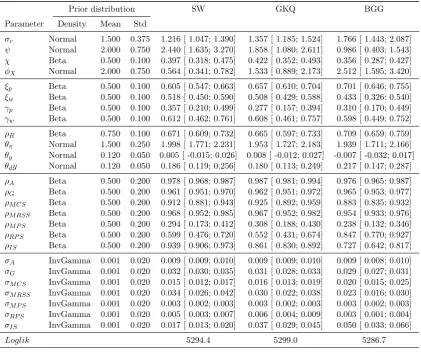
We estimate the models with Bayesian methods. For all three models we use the same

seven time series as observable variables as inSmets and Wouters(2007): the log difference

of real GDP, real consumption, real investment and the real wage, log hours worked, the

log difference of the GDP deflator, and the federal funds rate. We use US quarterly data

over the sample period 1966:1-2017:4.7 The parameter prior and posterior distributions are reported in Table D1in the Appendix, while further details on the estimation procedure

are given in AppendixD.

We calibrate several parameters in the estimation procedure that are hard to identify

in the models. We estimate the posterior distribution of the remaining 26 parameters,

which are common in all three models. The reason that all three models have the same

parameter vector estimated is to accommodate BMA in our exercise. BMA requires the

7_{We use the same sample asSmets and Wouters(2007) extended to the last full year observations are}

models to share the same set of observable variables, but the SW model has no empirical

implications for financial variables. Since parameters specific to the banking sector in the

GKQ or the BGG model are hard to identify without including financial variables among

the observable variables, we had to fix those parameters and estimate only parameters

common in all three models.

4.1 The workhorse New Keynesian model

Our first model follows closelySmets and Wouters(2007). It is a stochastic neoclassical

growth model augmented with price and nominal wage stickiness, price and nominal wage

indexation, habit persistence and investment adjustment costs. Household welfare in the

model is defined by their expected lifetime utility

Ω =E0

"_∞ X

t=0

βt[Ct−χCt−1]

1−σc

1−σc

exp

"

(σc−1) H_t1+ψ

1 +ψ ##

(7)

whereCtis real consumption,Htis hours supplied,βis the discount factor,χcontrols habit

formation, σc is the inverse of the elasticity of intertemporal substitution (for constant

labour), and ψ is the inverse of the Frisch labour supply elasticity. The monetary policy

rule for the nominal interest rateRn,t in the model is given by the Taylor-type rule

log

Rn,t

Rn

=ρrlog

Rn,t−1

Rn

+ (1−ρr)

θπlog

Πt

Π

+θylog

Yt Y

+θdylog

Yt Yt−1

+M P St, (8)

where Πtis inflation,Yt is real output, andM P St is a monetary policy shock that follows

an AR(1) process. The rest of the model is described in detail in AppendixA.

We review here the estimates for the parameters that are important for our policy

problem; the estimated posterior distribution for the rest of the parameters can be found

in Table D1 in the Appendix. The estimated Calvo parameter for price setting implies

that prices are updated on average every 2.07 quarters, but price indexation is rather

weak given that the indexation parameter is estimated to be lower than the prior mean.

Nominal wages are updated more frequently, on average every 1.67 quarters, but they are

original estimates of Smets and Wouters (2007) and correspond to the typical estimates

in the DSGE literature.

4.2 The banking model with outside equity

Our second model extends the SW model with a banking sector along the lines of

Gertleret al.(2012). In the model banks raise deposits and issue outside equity to finance

loans to firms. To motivate an endogenous constraint on the bank’s ability to raise funds,

Gertleret al.(2012) assume that the banker managing the bank may transfer a Θ fraction

of assets to their family. Hence, only 1−Θ fraction of assets can be pledged as collateral.

Recognizing this possibility, risk averse households limit the funds they lend to banks.

Our setup for the banking sector follows closely Gertler et al.(2012), and embeds in our

SW model in a similar fashion toGertler and Karadi(2011). For a detailed description of

the model see AppendixB.

The posterior distributions of the estimated parameters are close to the estimates in

the SW model. The only exceptions that are important for our policy problem are the

parameters characterizing intermediate firms’ price setting behaviour. Prices are updated

less frequently, on average every 2.91 quarters, but they are indexed to inflation more

weakly than in the SW model.

4.3 The financial accelerator model

Our third model extends the SW model with a banking sector along the lines of

Bernanke et al. (1999). In the model banks collect deposits and lend to entrepreneurs

who are subject to idiosyncratic shocks that affect their ability to repay their loans. The

financial market friction in this model, which is between the entrepreneur and the bank,

is driven by private information. Banks pool loans to protect themselves against credit

risk and charge a spread over the deposit rate. The household welfare function and the

Taylor-rule is the same as in the SW model. For a detailed description of the model see

AppendixC.

The posterior distributions of the estimated parameters resemble the estimates of the

SW model, but there a few notable exceptions that are important for our policy problem.

Nominal wages are more flexible and are updated on average every 1.76 quarters.

5

Model Weights

We estimate our models repeatedly with an increasing window of data, and compute

log predictive scores (4) and (5) for predictions made by our estimated models. Each

estimation sample starts at 1966:1. The first sample ends at 1970:4 (h= 20). We assess

our models based on how well they predict all seven observable variables jointly up to

four quarters ahead (K = 4).8 We increase the sample size by four quarters each time and repeat the same steps.9 Our last sample ends at 2016:4 (T = 208) as to allow for the computation of predictive densities using data up to 2017:4.

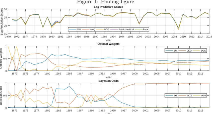
The top panel of Figure 1 shows the log predictive score function for each model.

These are similar across models throughout most of our sample period, indicating that

the predictive performance of all models is similar. There are exceptions to this at various

periods, for example from the mid 1990’s until the mid 2000’s (where the financial frictions

models dominate the SW model), and in the years around 1980 (where the SW model

does particularly well relative to the financial frictions models). Importantly, we employ

prediction pooling to aggregate the relative predictive performance differences over time.

The middle panel of Figure 1 shows the optimal prediction pool weights over the

sample period 1970:4-2017:4. To obtain these weights we solve the optimization problem

(6) recursively. At each point in time we use the log predictive scores up to that point to

determine the weights as if our full sample ended there. As is clear from the figure, the

BGG model predicts the best in the earlier part of the sample while in the later part of

the sample a larger weight is assigned to the SW model. Weights of approximately 42, 36

and 22 percent are assigned to the SW, BGG and GKQ models, respectively, by the end

of the sample period.

The bottom panel of Figure 1 shows an interesting contrast to the middle panel. It

shows how the Bayesian odds evolve over our sample, given a uniform prior belief of the

policy maker over the competing models. While for most of the sample period the GKQ

8_{We modify Dynare’s estimation routine to calculate the predictive densities.} 9

Figure 1: Pooling figure

1970 1972 1974 1976 1978 1980 1982 1984 1986 1988 1990 1992 1994 1996 1998 2000 2002 2004 2006 2008 2010 2012 2014 2016

Year

15 20 25 30

Log Predictive Scores

Log Predictive Scores

SW GKQ BGG Prediction Pool BMA

1972 1975 1977 1980 1982 1985 1987 1990 1992 1995 1997 2000 2002 2005 2007 2010 2012 2015

Year

0 0.5 1

Optimal Weights

Optimal Weights

SW GKQ BGG

1972 1975 1977 1980 1982 1985 1987 1990 1992 1995 1997 2000 2002 2005 2007 2010 2012 2015

Year

0 0.5 1

Bayesian Odds

Bayesian Odds

SW GKQ BGG

model provides the best fit and gets the highest odds, it receives much lower weight in

the optimal prediction pool. Had the policy maker used BMA to attach weights to the

models, he would have put most of her faith in the GKQ model while ignoring the other

two models entirely. In fact, with the exception of the years in the early 1990’s, BMA

have the tendency to assign almost zero weight to at least one model in our model pool.

Moreover, the optimal prediction pool weights seem to change slowly over time while large

changes in Bayesian odds can be brought by adding only a handful of observations to the

sample.

The difference in rankings across models between prediction pooling and BMA is due

to the standard trade-off between in-sample fit and out-of-sample predictive performance.

The financial frictions models fit the in-sample data quite well relative to the SW model

(and therefore have higher marginal log-likelihoods) yet they tend to predict poorly

(es-pecially in non-crises periods) in comparison to the SW model as they tend to over-fit

the data. As a result, the prediction pools assign a significant weight to the SW model.

Nevertheless, the situation is reversed at particular times (e.g. crisis times) when model

complexity may be beneficial for forecasting and therefore prediction pools should also

attach significant weight to the financial frictions models.

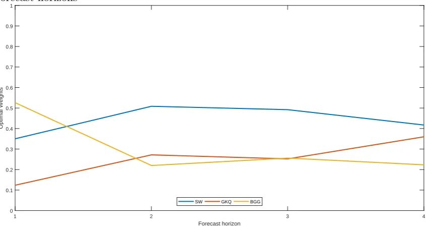
Figure 2: Optimal prediction pool weights at the end of our sample period using different forecast horizons

1 2 3 4

Forecast horizon

0 0.1 0.2 0.3 0.4 0.5 0.6 0.7 0.8 0.9 1

Optimal Weights

SW GKQ BGG

end of our sample period depend on the forecast horizons used. Irrespective of the forecast

horizon used, all three models are useful in terms of predictability and ought to be

em-ployed by a policy maker when designing policy even though the forecasting performance

of the GKQ and BGG models are inferior to the SW model at most horizons.

Overall, our results suggest that if the policy maker does not believe any model to be

correct, she must nevertheless be much more cautious in rejecting models that appear to

be inferior. The intuition here is that such models while not particular accurate most of

the time, may well be very useful some of the time, and thus the optimal policy should take

this into consideration rather than rejecting the use of such models. Moreover, prediction

pooling is a far more robust method for attaching weight to models as these are more robust

to outliers and therefore evolve more smoothly over time than corresponding weights from

BMA.

6

Optimal Robust Rules

This section analyses the optimal simple rules for our model economies. First, we define

the different types of optimal simple rules we compute. Then, we examine optimal simple

using different ways to attach weights to models. Finally, we examine the welfare cost of

suboptimal policy using two different sets of criteria: i) the cost of implementing the rule

designed for model i in the environment of model k6=iand ii) the cost of implementing

a rule with deviations from the optimal parameter values.

6.1 Computation and Welfare Measures

We seek policy parameters ρ=hρr απ αy αdy

i

in the Taylor-rule

log

Rn,t

Rn

=ρrlog

Rn,t−1

Rn

+απlog

Πt

Π

+αylog

Yt Y

+αdylog

Yt Yt−1

(9)

that maximize the unconditional lifetime utility of households. We estimate the model

using the same form of the Taylor-rule (8) and the same priors on its parameters as in

Smets and Wouters(2007). However, we reparametrize the feedback coefficients by setting

απ = (1−ρr)θπ, αy = (1−ρr)θy, and αdy = (1−ρr)θdy to allow for the possibility of a

price level rule (ρr= 1) when computing optimized simple rules.

We evaluate policies by computing the welfare in model iassociated with a particular

policy rule. Let

Ωi(ρ, ψi) =E0

"_∞ X

t=0

βtU(Ct(ρ, ψi), Ht(ρ, ψi))

#

ψi ∈Ψi (10)

denote the unconditional lifetime utility of households from a second-order approximation

around a deterministic steady state in model M_i conditional on a particular rule ρ and

a parameter vector ψi. Then given weights {wi}mi=1, the policy maker seeks a rule ρ∗

common to every model in the pool that maximizes

¯

Ω(ρ, w) =

m X i=1 wi Z Ψi

Ωi(ρ, ψi)p(ψi|YoT,Mi)dψi ≈ m X i=1 wi N X j=1

Ωi(ρ, ψi,j). (11)

where ψi,j is a draw from parameter space Ψi. The optimization problem defined by

maximizing (11) can incorporate both awithin-model robustness, by averaging ofN draws for each modelMi and anacross-model robustness by using a weighted average of model

specific welfare measures. Calculation of (11) is numerically facilitated by MCMC methods

Markov chain. Thus, the integral can be approximated by a sum.

We compute two types of optimal simple rules which we will refer to as robust

opti-mal simple rules and mean optiopti-mal simple rules. Robust optiopti-mal simple rules incorporate

both within- and across-model uncertainty. For each model i, we draw N = 500

param-eter vectors ψi,j, j ∈ [1, N] from the estimated posterior distributions of each model to

approximate the integral above. Mean optimal simple rules on the other hand are based

on a single parameter vector (N = 1). They are computed by fixing the parameter vector

at the estimated posterior mean of each model. Comparing the two types of rules allows

us to assess what happens if the policy maker ignores within-model uncertainty in the

policy design.

We compare alternative policies in terms of consumption equivalent welfare changes.

Consider two alternative policies ρ1 and ρ2. The consumption equivalent welfare cost of

adopting ρ2 in model Mi is the fraction ωi of the consumption stream households are

willing to give up to be as well off under ρ2 as under ρ1. It is implicitly defined by the

indifference condition

Ωi(ρ2, ψi) =E0

"_∞ X

t=0

βtU((1−ωi)Ct(ρ1, ψi), Ht(ρ1, ψi))

#

(12)

This welfare measure allows us to compare the effect of the same policy in different model

economies directly or aggregate the effect of the policy across models. To compute the

welfare cost of a policy rule common to all models in a pool, we calculate the weighted

average of the associated welfare cost from each model using the weights assigned to each

model

ω =

3

X

i=1

wiωi (13)

6.2 Optimal Within-model Robust Rules

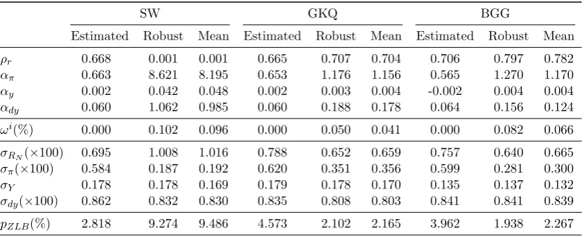
Table2compares three policy rules and their outcomes for each of the three models in

our prediction pool. The first is the estimated rule which are very similar across models.

The second is the robust optimal simple rule in the ‘Robust’ column and the third in the

‘Mean’ column is the mean optimal simple rule.

rule. The sub-optimality of the estimated rules is well-established in the literature. Our

consumption-equivalent measure ωi indicates that using either the robust or the mean

optimized rules provides a welfare gain over the estimated rule ranging from around 0.05

percent for the GKQ model to 0.10 percent for the SW model.

The two types of optimal simple rules are very similar. The small difference between

them suggests that ignoring within-model uncertainty has only a small impact. The

dif-ference between the welfare gains of the robust and the mean optimal simple rules over

the estimated rules shows that if the policy maker ignores within-model uncertainty, then

she underestimates the gains from optimal policy for each model. Moreover, when we

compare the robust and the mean optimal simple rules to each other directly we find that

the welfare cost associated with the mean optimal simple rule is about ten-thousandth of

one percent of consumption.10 Comparing the welfare gains associated with the robust and mean optimal simple rules reported in Table2directly is misleading. The welfare gain

in the ’Mean’ columns shows the fraction of the consumption stream households need to

be given to be indifferent between the mean optimal simple rule and the rule fixed at the

estimated posterior mean. The welfare gain of the robust optimal simple rule, on the other

hand, is computed as the average welfare gain of the robust optimal simple rule across

the N = 500 parameter vector draws from the estimated posterior distributions of each

model. Hence, the differences in the welfare gains reported in Table 2reflect the effect of

within-model uncertainty on the estimated rule and not on the optimal rule.11

Across-model differences of optimal rules are considerable. The optimal simple rules,

both robust and mean, designed for the SW model are close to a pure inflation targeting

rule. They have almost zero interest rate smoothing parameter ρr but see a very

ag-gressive immediate response to changes in inflation captured by the feedback parameter

απ.12 Consequently, the welfare gains are closely related to the large decrease in inflation

volatility implied by the optimal rules: the standard deviation of inflation decreases by

a factor of three from 0.00584 to 0.00187. By contrast the optimal rules for the GKQ

and BGG models have considerable interest rate smoothing but far more muted response

10_{The welfare cost associated with the mean optimal simple rule is 0.16, 0.54 and 1.87 ten-thousandth}

of one percent of consumption in the SW, GKW and BGG models, respectively.

11

This difference is due to Jensen’s inequality given that the welfare function is concave.

12_{We do not impose an upper bound on the policy parameter α}

π during optimization. Imposing the

upper boundαπ≤3 as inSchmitt-Grohe and Uribe(2007) for example would reduce the welfare gain for

to inflation. The welfare gains from decreased inflation volatility, which works through

agents’ inflation expectations, are much smaller.

The lack of interest rate smoothing in the optimal policy for the SW model results

in a higher nominal interest rate volatility than under the estimated rule. An important

consequence of the wider interest rate distribution is that the unconditional probability

of hitting the zero lower boundpZLB is much higher than with the estimated policy rule–

over 9 percent per quarter or about once every 3 years.13 This contrasts with about 2 percent per quarter for the optimal rules in the GKQ and BGG models, or about once

every 12.5 years. Available data suggest that zero lower bound episodes are rare but

long-lived (Dordal-i-Carreras et al., 2016a). The U.S. post-WWII experience (seven years at

the zero lower bound over seventy years) indicates that unconditional probabilities below

10 percent are empirically plausible. However, a policy maker may want to set an upper

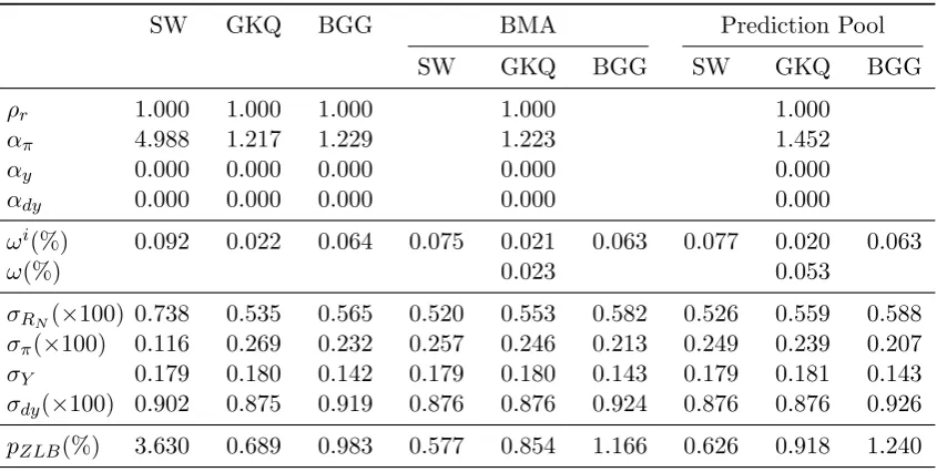
bound on this probability as part of the policy mix.

6.3 Optimal Across-model Robust Rules

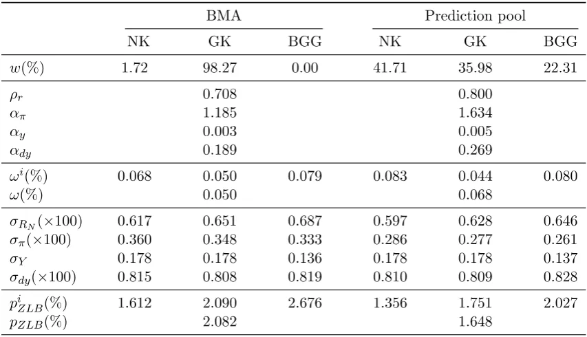
We now turn to optimal across-model optimal rules. We compare two sets of policy

rules computed using two different set of pooling weights. The first uses BMA and the

second we call ‘Prediction Pool’ uses optimal prediction pool weights.14 Table3shows the results for robust optimal simple rules which incorporate both across-model and

within-model uncertainty. The mean optimal simple rules, which are only across-within-model robust

with parameters in each model set at their estimated posterior means and are very similar

to the robust simple rules, are reported in TableE3 in the Appendix.

The contribution of within-model robustness, just like in the case of individual models

in the previous section, seems small regardless of which sets of weights we use to account

for across-model uncertainty. Comparing the welfare gains from robust and mean optimal

simple rules shows again that the policy maker underestimates the gains from optimal

policy if within-model uncertainty is ignored. But the resulting optimal rules are very

13

The unconditional probability of hitting the zero lower bound is computed from a normal approxima-tion of the gross nominal interest rate’s ergodic distribuapproxima-tion. LetRN and σRN denote the deterministic

steady state and the unconditional standard deviation of the gross nominal interest rate, respectively, computed from a second-order approximation around a deterministic steady state. Then the probability of hitting the zero lower bound, pZLB is given by the probability that the gross nominal interest rate is

below one in the normal distributionN(RN, σRN).

14_{We have also experimented with an equally weighted pool, but the results are very close to those}

Table 2: Optimized simple rules

SW GKQ BGG

Estimated Robust Mean Estimated Robust Mean Estimated Robust Mean

ρr 0.668 0.001 0.001 0.665 0.707 0.704 0.706 0.797 0.782

απ 0.663 8.621 8.195 0.653 1.176 1.156 0.565 1.270 1.170

αy 0.002 0.042 0.048 0.002 0.003 0.004 -0.002 0.004 0.004

αdy 0.060 1.062 0.985 0.060 0.188 0.178 0.064 0.156 0.124

ωi_{(%) 0.000 0.102 0.096 0.000 0.050 0.041 0.000 0.082 0.066}

σRN(×100) 0.695 1.008 1.016 0.788 0.652 0.659 0.757 0.640 0.665

σπ(×100) 0.584 0.187 0.192 0.620 0.351 0.356 0.599 0.281 0.300

σY 0.178 0.178 0.169 0.179 0.178 0.170 0.135 0.137 0.132

σdy(×100) 0.862 0.832 0.830 0.835 0.808 0.803 0.841 0.841 0.839

pZLB(%) 2.818 9.274 9.486 4.573 2.102 2.165 3.962 1.938 2.267

Note: The simple rules in the ’Robust’ column are optimal robust simple rules based on 500 draws from the estimated posterior distribution of each model. Every variable in the column is computed for each draw then averaged across draws. The simple rules in the ’Mean’ column are optimal simple rules computed at the estimated posterior mean of each model. ωi shows the fraction

of the consumption stream households need to give up to have the same welfare as under the estimated rule. σRN, σΠ, σY, and σdY denote the unconditional standard deviation of the gross

nominal interest rate, the inflation rate, output and output growth computed from a second-order approximation around a deterministic steady state. Some of the standard deviations are scaled by 100 for ease of presentation. pZLB is the probability that the gross nominal interest rate is below

one in the normal distribution N(RN, σRN), where RN is the deterministic steady state of the

nominal interest rate.

similar in Tables3andE3and ignoring within-model uncertainty has only a small impact.

A direct comparison of the robust and mean optimal simple rules to each other reveals

that that the welfare cost associated with the mean optimal simple rule is again about

ten-thousandth of one percent of consumption.15

The choice of pooling weights matters for the optimized rule. The optimal simple rule

obtained using the optimal prediction pool weights implies a higher welfare gain over the

estimated rule compared to the policy rules obtained using the BMA weights. This higher

welfare gain is explained by a combination of two factors: differences in i) the weights

and ii) in the rules. The first is a composition effect since the weights used in (13) to

aggregate the welfare gains from the individual models are different. If we aggregated

the welfare gains of the prediction pool optimal rule from the individual models using the

BMA weights, then the aggregate welfare gain would be 0.045 only. Hence, differences in

15

the optimal rules would imply a higher difference in welfare gains were the weights the

same.

The second factor is the differences in the rules themselves. Using the optimal

predic-tion pool weights implies a more persistent policy rule that also responds more aggressively

to changes in inflation and output growth compared to the policy rules obtained using the

BMA weights. The welfare gains from the individual models in theωi row reveal that the

prediction pool rule trades-off welfare gains from the GKQ model for welfare gains from

the SW model given that it attaches more weight to the latter. Interestingly, inflation

volatility is reduced in all three models the most by the prediction pool optimal rule, but

the likely welfare gains from this reduced volatility are partly negated by the interest rate

smoothing parameter being above its optimal level in all three models.

Finally, across-model robustness removes the high probability of hitting the nominal

interest rate lower bound seen in Table2for the SW model with only within-model

robust-ness. Since the optimal values for the interest rate smoothing parameter are well above

the estimated values regardless of the weights we use, interest rate volatility decreases for

every optimal policy and so does the probability of hitting the zero lower bound.

6.4 The Welfare Cost of Suboptimal Policy

In this section we examine the welfare cost of suboptimal policy using two different

sets of criteria. First, we quantify the cost of implementing the rule designed for modeli

in the environment of modelj6=i. Then, we analyse the cost of implementing a rule with

deviations from the optimal parameter values.

Table4shows the welfare cost of using a rule optimized for a specific model in another

model. This is a counterfactual exercise that shows the cost of incorrectly identifying

the data generating process. For example, if we use the robust simple rule optimized for

the SW model in the BGG model, then the welfare loss is 0.052 percent of consumption

relative to the robust simple rule optimized for the BGG model itself. The results confirm

that that the robust simple rule optimized for the GKQ and BGG models are very similar,

and they both are very different from the robust simple rule optimized for the SW model.

Using the rule optimized for the GKQ model in the BGG model, or vice versa, imply very

Table 3: Optimized robust simple rules

BMA Prediction pool

NK GK BGG NK GK BGG

w(%) 1.72 98.27 0.00 41.71 35.98 22.31

ρr 0.708 0.800

απ 1.185 1.634

αy 0.003 0.005

αdy 0.189 0.269

ωi(%) 0.068 0.050 0.079 0.083 0.044 0.080

ω(%) 0.050 0.068

σRN(×100) 0.617 0.651 0.687 0.597 0.628 0.646

σπ(×100) 0.360 0.348 0.333 0.286 0.277 0.261

σY 0.178 0.178 0.136 0.178 0.178 0.137

σdy(×100) 0.815 0.808 0.819 0.810 0.809 0.828

pi_ZLB(%) 1.612 2.090 2.676 1.356 1.751 2.027

pZLB(%) 2.082 1.648

Note: The robust optimal simple rules in the table are based on 500 draws from the estimated posterior distribution of each model. Every variable in the table is computed for each draw then averaged across draws. ωi shows the fraction of the consumption stream households need to give

up to have the same welfare as under the estimated rule in ach model. σRN, σΠ, σY, and σdY

denote the unconditional standard deviation of the gross nominal interest rate, the inflation rate, output and output growth computed from a second-order approximation around a deterministic steady state. Some of the standard deviations are scaled by 100 for ease of presentation. pZLB

is the probability that the gross nominal interest rate is below one in the normal distribution

N(RN, σRN), where RN is the deterministic steady state of the nominal interest rate.

two models, however, implies much larger welfare losses than the other way around. This

explains why the robust simple rule optimized for the prediction pool is so close to the

rule optimized for the GKQ and BGG models. The final row shows the welfare cost of

using the robust rule optimized for the prediction pool in Table 3 relative to the model

specific robust optimal rules reported in Table 2. These now avoid the large costs of the

single model optimized rules and the costs are generally small relative to the gains from

using optimal rules.

Figure 3 shows how sensitive welfare is to changes in the coefficients in the robust

optimal simple rule in each model. Each panel in the graph shows the consumption

equivalent variation in welfare when changing a single parameter in the robust optimal

Table 4: Welfare cost of robust optimal policyiin model j6=i

SW GKQ BGG

SW 0.000 0.140 0.052

GKQ 0.035 0.000 0.003

BGG 0.028 0.002 0.000

Pool 0.019 0.006 0.001

Note: The table shows what happens when an optimal simple rules optimized for modeli is used in modelj6=i. The first column shows the consumption equivalent welfare loss in the SW model relative to the welfare attained using the robust simple rule optimized for the SW model if, for example, we use the robust simple rules optimized for the SW, GKQ, BGG models, respectively. The last row shows the welfare cost incurred in modeliwhen instead of using the robust simple rule optimized for modeliwe use the robust optimal simple rule obtained with the optimal prediction pool weights.

of changing a parameter in the Taylor rule, while each row shows the welfare costs of

deviating from the optimal parameter values in a given model.

In the SW model welfare is quite flat around the optimal point along every dimension.

Deviations have small effects and welfare is most sensitive to changes in the output

feed-back parameterαy.16 In the financial friction models deviations from the optimal valueαy

still dominate the policy maker’s objective: deviations can have large welfare consequences

that can reach as much as a 5% consumption equivalent. However, welfare in those models

is also very sensitive to deviations of the interest rate smoothing parameter, ρr, from its

optimal value. The panels in the last row show the welfare cost of deviating from the

optimal parameter values of the common robust rule in all three models at the same time

optimized for the prediction pool. These panels are essentially weighted averages of the

three panels above them using the weights assigned to each model in the prediction pool.

The numbers here are considerably smaller than in the second and third rows due to the

fact that the SW model receives the largest weight in the prediction pool.

6.5 A Price Level Rule

Our results then show that even small deviations of ρr and αy have serious welfare

consequences with losses far greater than any gains relative to the estimated rule reported

so far. So suppose that the monetary policymaker commits to a rule with ρr = 1 and

0 0.2 0.4 0.6 0.8 0 1 2 SW 10-3

4 6 8 10 12

0 5 10

10-3

0 0.1 0.2 0.3 0.4 0

5 10 15

10-3

0.5 1 1.5

0 2 4 6 8 10-4

0 0.2 0.4 0.6 0.8 0

0.5 1

GKQ

1 1.2 1.4 1.6 1.8 2 0

5 10 15

10-3

0 0.1 0.2 0.3 0.4 0

2 4 6

0 0.2 0.4 0.6 0.8 1 0

0.05 0.1

0 0.2 0.4 0.6 0.8 0 0.2 0.4 0.6 0.8 BGG

1 1.2 1.4 1.6 1.8 2 0 2 4 6 8 10-3

0 0.1 0.2 0.3 0.4 0

1 2 3

0 0.2 0.4 0.6 0.8 1 0

0.05 0.1

0 0.2 0.4 0.6 0.8

R

0 0.05 0.1

Pool

1 1.2 1.4 1.6 1.8 2 0

5 10 15

10-3

0 0.1 0.2 0.3 0.4

y

0 0.5 1 1.5

0 0.2 0.4 0.6 0.8 1

dy

0 0.02 0.04

Figure 3: The cost of bad policy I

2 4 6 8 0 0.005 0.01 0.015 0.02 0.025 0.03 0.035 SW

1 1.2 1.4 1.6 1.8 2 0

5 10 15 10

-3 GK

1 1.2 1.4 1.6 1.8 2 0 2 4 6 8 10 10 -3 BGG

1 1.2 1.4 1.6 1.8 2 0 1 2 3 4 5 6 7 8

10-3 Prediction pool

Figure 4: The cost of bad policy II

Note: The graph shows the welfare cost of deviating from the optimal value ofαπin in the optimal

robust price level rule. Price level rules use the restrictionρr = 1 and αy =αdy = 0. The first

three panel show the welfare cost of deviating from the robust price level rule optimized for that particular model. The last panel shows the welfare cost of deviating from the common robust price level rule in all three models at the same time optimized for the prediction pool. Welfare costs are measured in consumption equivalent welfare changes. The vertical red line shows the optimal value of the parameter that is changed in each column.

αy =αdy= 0. Then integrating (9) and putting Π_Πt = P_P¯t_t/P_/P¯_tt−₋1₁ where ¯Pt is the price trend

in the constant inflation rate steady state, we arrive at the rule

Rn,t Rn

=απ Pt

¯

Pt

(14)

which is aprice-level rule that adjusts the deviation of the nominal interest rate to changes in the price level relative to its long-run trend. The benefits of price-level targeting versus

inflation targeting have been studied in the literature now for some time. (See, for example,

Svensson (1999), Schmitt-Grohe and Uribe (2000), Vestin (2006), Gaspar et al. (2010),

Giannoni (2014)). These papers examine the good determinacy and stability properties

of price-level targeting. Holden(2016) shows these benefits extend to a ZLB setting. The

intuition for the benefits of price-targeting is as follows: faced with of an unexpected

temporary rise in inflation, price-level stabilization commits the policymaker to bring

inflation below the target in subsequent periods. In contrast, with inflation targeting, the

drift in the price level is accepted.

Our results in Table 5 and Figure4 indicate a further benefit of price-level targeting:

when the robust rule is implemented, even with departures from its optimal setting of the

single feedback parameterαπ that defines the policy, it remains robust across models with

Table 5: Optimized simple robust price level rules

SW GKQ BGG BMA Prediction Pool

SW GKQ BGG SW GKQ BGG

ρr 1.000 1.000 1.000 1.000 1.000

απ 4.988 1.217 1.229 1.223 1.452

αy 0.000 0.000 0.000 0.000 0.000

αdy 0.000 0.000 0.000 0.000 0.000

ωi(%) 0.092 0.022 0.064 0.075 0.021 0.063 0.077 0.020 0.063

ω(%) 0.023 0.053

σRN(×100) 0.738 0.535 0.565 0.520 0.553 0.582 0.526 0.559 0.588 σπ(×100) 0.116 0.269 0.232 0.257 0.246 0.213 0.249 0.239 0.207

σY 0.179 0.180 0.142 0.179 0.180 0.143 0.179 0.181 0.143

σdy(×100) 0.902 0.875 0.919 0.876 0.876 0.924 0.876 0.876 0.926

pZLB(%) 3.630 0.689 0.983 0.577 0.854 1.166 0.626 0.918 1.240

Note: Simple price level rules use the restriction ρr = 1 and αy =αdy = 0 and only the value

of απ is optimized. All rules in the table are based on 500 draws from the estimated posterior

distribution of each model. Every variable in the column is computed for each draw then averaged across draws. ωishows the fraction of the consumption stream households need to give up to have

the same welfare as under the estimated rule in each model. σRN, σΠ, σY, and σdY denote the

unconditional standard deviation of the gross nominal interest rate, the inflation rate, output and output growth computed from a second-order approximation around a deterministic steady state. Some of the standard deviations are scaled by 100 for ease of presentation. pZLB is the probability

that the gross nominal interest rate is below one in the normal distributionN(RN, σRN), where RN is the deterministic steady state of the nominal interest rate.

7

Conclusion

This paper studies the problem of designing robust simple rules when the policy maker

has at her disposal a finite set of models, none of which are believed to be the true

data generating process. We assign weights to models on the basis of the accuracy of

their 4-period ahead forecasts rather than their in-sample fit, consistent with the

forward-looking viewpoint of the policy maker. We study the robust optimal policy problem

in the form of an optimized Taylor-type nominal interest rate rule under this weighting

scheme using three estimated models exemplifying the policy makers’ uncertainty about

how to incorporate financial frictions into the canonical DSGE model ofSmets and Wouters

(2007). In comparison with Bayesian model averaging, we find that our prediction pool

choice has a significant impact on the robust optimized rule.

policy design problem. It only requires models to share the same policy instrument, to

provide a k-period ahead predictive density given macro-economic data, and to have a

welfare criterion to rank alternative policies. The models in the pool do not need to share

the estimated parameter vector, nor even the observables; they can be nested as well as

non-nested. Thus, the methodology can be applied to a wide range of macroeconomic

models from mainstream DSGE, behavioural to agent-based, and indeed to other

non-macroeconomic settings as long as these three requirements are met.

Several open questions offer possible avenues for further research. First, our policy

problem can be extended to accommodate macro-prudential instruments where banks are

subjected to a common capital, or equivalently leverage-ratio, requirement.

Second, whereas the results we have obtained in the paper examine the possibility of

a hitting a zero-lower bound for monetary policy, they are not designed to minimize this

outcome as in Levine et al. (2012). In a recent paper Dordal-i-Carreras et al. (2016b)

demonstrate that a regime switching representation of risk premium shocks can generate

a realistic distribution of zero-lower bound durations in a standard New Keynesian model.

Incorporating zero-lower bound considerations into our policy problem may reveal policy

trade-offs that are not present in our results.

Third, we have confined our study to one standard form of interest rate rule responding

with interest rate inertia to inflation, output and output growth. This nested a price level

rule which many papers in the literature have found to have good robustness properties.

Other rules, such as wage inflation targeting, need to be explored.

Fourth an aspect of the robustness approach, largely ignored by the literature, is the

scope for expectation differences between private and public sectors. There is a need

to consider the possibility that the private sector may also believe there are competing

models. By assuming that each model has RE with model-consistent expectations our

application has ruled out this possibility. This case of model-inconsistent expectations

needs to be factored into truly robust Bayesian rules. An alternative is to pursue a

behavioural approach and drop the RE assumption altogether.17

Fifth, the use of real-time data when analysing the out-of-sample forecast performances

of competing models to compute weights would be an interesting exercise. An application

of density forecasting using real time data, but without model pooling, is provided by

McAdam and Warne(2019). Another important technical issue that may arise is that the

state space over which the two models are stable may not coincide. This is a problem as

then in both the determination of the optimal pool and the robust optimal policy, one

model may be favoured over the other.

References

Adalid, R., Coenen, G., McAdam, P., and Siviero, S. (2005). The Performance and

Robustness of Interest-Rate Rules in Models of the Euro Area. International Journal of Central Banking,1(1), 95–132.

Bernanke, B., Gertler, M., and Gilchrist, S. (1999). The Financial Accelerator in

Quanti-tative Business Cycles. In M. Woodford and J. B. Taylor, editors,Handbook of Macroe-conomics, vol. 1C. Amsterdam: Elsevier Science.

Bernardo, J. and Smith, A. (1994). Bayesian Theory. Wiley, Chichester, UK.

Binder, M., Lieberknecht, P., Quintana, J., and Wieland, V. (2017). Model Uncertainty

in Macroeconomics: On the Implications of Financial Frictions. C.E.P.R. Discussion

Papers.

Binder, M., Lieberknecht, P., Quintana, J., and Wieland, V. (2018). Robust

Macropruden-tial Policy Rules under Model Uncertainty. Annual Conference 2018, German Economic

Association.

Brock, W. A., Durlauf, S. N., and West, K. D. (2007a). Model uncertainty and policy

evaluation: Some theory and empirics. Journal of Econometrics,127(2), 629–664. Brock, W. A., Durlauf, S. N., Nason, J. M., and Rondina, G. (2007b). Simple versus

optimal rules as guides to policy. Journal of Monetary Economics,54(5), 1372–1396. Calvert Jump, R. and Levine, P. (2019). Behavioural New Keynesian Models. Journal of

Macroeconomics,59(C), 59–77.

Chamberlain, G. (2000). Econometric Applications of Maximin Expected Utility. Journal of Applied Econometrics,15, 625–644.

Christiano, L. L., Eichenbaum, M., and Evans, C. L. (2005). Nominal rigidities and the

dynamic effects of a shock to monetary policy. Journal of Political Economy, 113(1), 1–45.

Cogley, T. and Sargent, T. (2005). The conquest of U.S. inflation: learning and robustness

to model uncertainty. Review of Economic Dynamics,8(2), 528–563.

Cogley, T., De Paoli, B., Matthes, C., Nikolov, K., and Yates, T. (2011). A Bayesian

approach to optimal monetary policy with parameter and model uncertainty. Journal of Economic Dynamics and Control,35(12), 2186–2212.

Cˆot´e, D., Kuszczak, J., Lam, J.-P., Liu, Y., and St-Amant, P. (2004). The Performance

and Robustness of Simple Monetary Policy Rules in Models of the Canadian Economy.

Canadian Journal of Economics,37(4), 978–998.

Del Negro, M., Hasegawa, R., and Schorfheide, F. (2016). Dynamic Prediction Pools: An

Investigation of Financial Frictions and Forecasting Performance. Journal of Economet-rics, 192, 391–405.

Dennis, R., Leitemo, K., and Soderstrom, U. (2009). Methods for Robust Control.Journal of Economic Dynamics and Control,33(8), 1604–1616.

Dordal-i-Carreras, M., Coibion, O., Gorodnichenko, Y., and Wieland, J. (2016a).

Infre-quent but Long-Lived Zero-Bound Episodes and the Optimal Rate of Inflation. NBER

Working Papers 22510, National Bureau of Economic Research, Inc.

Dordal-i-Carreras, M., Coibion, O., Gorodnichenko, Y., and Wieland, J. (2016b).

Infre-quent but Long-Lived Zero-Bound Episodes and the Optimal Rate of Inflation. NBER

Working Papers 22510, National Bureau of Economic Research, Inc.

Ellison, M. and Sargent, T. J. (2012). A Defense Of The FOMC. International Economic Review,53(4), 1047–1065.

Gaspar, V., Smets, F., and Vestin, D. (2010). Is Time Ripe for Price Level Path Stability?