The influence of phase-locking on internal resonance from a nonlinear normal mode perspective

(1)

The in

ﬂ

uence of phase-locking on internal resonance

from a nonlinear normal mode perspective

T.L. Hill

a,n

, S.A. Neild

a

, A. Cammarano

b

, D.J. Wagg

c a

Department of Mechanical Engineering, University of Bristol, Bristol BS8 1TR, UK b

School of Engineering, University of Glasgow, Glasgow G12 8QQ, UK c

Department of Mechanical Engineering, University of Shefﬁeld, Shefﬁeld S1 3JD, UK

a r t i c l e i n f o

Article history:

Received 18 December 2015 Received in revised form 24 March 2016 Accepted 16 May 2016 Handling Editor: W. Lacarbonara Available online 6 June 2016

Keywords: Internal resonance Nonlinear normal modes Backbone curves Nonlinear dynamics Cable dynamics

a b s t r a c t

When a nonlinear system is expressed in terms of the modes of the equivalent linear system, the nonlinearity often leads to modal coupling terms between the linear modes. In this paper it is shown that, for a system to exhibit an internal resonance between modes, a particular type of nonlinear coupling term is required. Such terms impose a phase condition between linear modes, and hence are denotedphase-lockingterms. The effect of additional modes that are not coupled via phase-locking terms is then investi-gated by considering the backbone curves of the system. Using the example of a two-mode two-model of a taut horizontal cable, the backbone curves are derived for both the case where phase-locked coupling terms exist, and where there are no phase-locked coupling terms. Following this, an analytical method for determining stability is used to show that phase-locking terms are required for internal resonance to occur. Finally, the effect of non-phase-locked modes is investigated and it is shown that they lead to astiffeningof the system. Using the cable example, a physical interpretation of this is provided.

&2016 The Authors. Published by Elsevier Ltd. This is an open access article under the CC BY license (http://creativecommons.org/licenses/by/4.0/).

1. Introduction

Weakly nonlinear systems typically have an underlying linear structure and the underlying linear modes are often used to describe the fundamental components of the system. In this paper we investigate the coupling terms that are present in nonlinear systems when projected onto these linear modes. Specifically, we show how phase-locking conditions in these terms influence the internally resonant dynamic behaviour. Such phenomena are often observed in forced, lightly damped, and weakly nonlinear systems with multiple degrees-of-freedom, which represent a variety of physical applications, see for example[1–4]. Here, internal resonance is defined as the triggering of a dynamic response of a linear mode of the system that is not subjected to direct external excitation. Many previous authors have considered problems of this type, see for example[3,4]and references therein.

In this work we will use the normal form technique proposed by [5]for multi-degree-of-freedom forced, damped,

weakly nonlinear systems. This approach leads naturally to the analysis of backbone curves, which deﬁne the dynamic behaviour of periodic motions in the unforced and undamped equivalent system, in the amplitude vs frequency plane. These are equivalent to the loci of the nonlinear normal modes (NNMs), represented in the amplitude vs frequency projection.

Contents lists available atScienceDirect

journal homepage:www.elsevier.com/locate/jsvi

Journal of Sound and Vibration

http://dx.doi.org/10.1016/j.jsv.2016.05.028

0022-460X/&2016 The Authors. Published by Elsevier Ltd. This is an open access article under the CC BY license (http://creativecommons.org/licenses/by/4.0/).

n_{Corresponding author.}

(2)

Many authors have considered the NNMs of, for example, a two-degree-of-freedom spring–mass system [6–8]. Lewan-dowski[9]pointed out that bifurcations can occur in the backbone curves of this type, and the same author went on to analyse beam, membrane and plate examples[10]. More recently, the current authors have used backbone curves to study internal resonance phenomena in systems of coupled nonlinear oscillators[11–14]. In particular, bifurcations of backbone curves were used to indicate where an internal resonance may by triggered, however additional solution branches have also been observed that do not trigger internal resonances. As internal resonance is deﬁned here as a behaviour seen in systems subject to external excitation, and as the backbone curves describe the unforced and undamped responses, it should be noted that the backbone curves themselves do not exhibit internal resonance. However, backbone curves do uncover modal interactions which may lead to internal resonances when external forcing and damping are introduced.

Here, the phenomenon of phase-locking between modes during internal resonance is considered in detail. Much of this discussion is motivated by the example of a taut cable, introduced inSection 2. Expressions for the backbone curves of the cable are developed inSection 3by considering the interactions between pairs of linear modes. This analysis reveals that, depending on the pairs of modes that are considered, the backbone curves are either phase-locked or phase-unlocked.

One significant feature of phase-locking is revealed inSection 4, where it is shown that phase-locked terms are required for internal resonance. This is demonstrated using an analytical stability analysis, which considers the stability of the zero-amplitude solution of an unforced linear mode of a general weakly nonlinear system. This general analysis is applied to the cable example, demonstrating the physical significance of this observation. Lastly, inSection 5, the cable example is used to investigate the influence of additional, phase-unlocked, modes on the dynamic behaviour of an internally resonant pair of modes. It is shown that, although this type of mode cannot lead to additional internal resonances, they can impose a stiffening effect on the system, altering the response of the phase-locked pair. For the cable, this effect can be explained physically as an increase in the axial tension in the cable, due to the presence of additional modal oscillations.

2. Resonant equations of motion

Weakly nonlinear, multi-degree-of-freedom systems are often expressed in terms of the modal coordinates for the linearised version of the system, as the linear terms will then be decoupled. However, decoupling of the nonlinear terms is typically not achieved via a linear modal transform, and hence the modes will not, in general, match the NNMs of the

nonlinear system. Note that here we use the termmodes to refer to the modes of the linearised system. A multimodal

nonlinear system may be written in modal coordinates,q, as

€

qþ

_Γ

q_þ

_Λ

qþNðqÞ ¼f: (1)

Assuming linear modal damping, thekth diagonal elements in diagonal matrices

Γ

and

Λ

are 2

ζ

k

ω

nkand

ω

nk 2

respectively and the vectorNcontains the nonlinear stiffness terms, andfrepresents the external excitation vector in modal coordinates. Here,

ζ

kand

ω

nkare used to denote the linear damping ratio and linear natural frequency of thekth mode respectively.

To analyse weakly nonlinear systems it is helpful to transform the equations of motion into a new set of coordinates,u, which describe only the resonant components of the response. The dynamic equation inuis termed theresonantequation of motion. This can then be used toﬁnd steady-state solutions, in terms of modal amplitudes, via an exact harmonic balance using trial solutions of the form

uk¼Ukcos

ω

rkt

ϕ

k

¼Uk 2 e

jðωrktϕkÞ þUk 2 e

jðωrktϕkÞ ¼_u

pkþumk; (2)

.

If forcing is near-resonant, i.e. the frequency of the forcing acting on any mode is close to the natural frequency of that mode, or if there is no forcing, then the resonant equation of motion is found by applying a nonlinear near-identity transform to Eq.(1)to give

€

qþ

_Γ

q_þ

_Λ

qþNðqÞ ¼f⟶q¼uþhðuÞ u€þ

_Γ

u_þ

_Λ

uþNuðuÞ ¼f; (3)

where his a vector of harmonic components. In the formulation shown in Eq. (3), it is assumed that the forcing and

(3)

2.1. Resonant equations of the example system

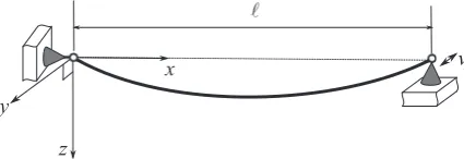
As an example we consider the dynamics of a horizontal taut cable, shown schematically inFig. 1. This is described using the modal equations of motion, derived in[16]and discussed in detail in[4], which include gravitational sag and tension effects. The dynamics for thekth in- and out-of-plane modes, denotedzkandykrespectively (where in-plane relates to the plane in which gravitational sag occurs with the sag acting in the positive direction) may be expressed as

€

zkþ2

ζ

k

ω

nkz_kþ

ω

2nkzkþ

X1

i¼1

ν

ki

mzk y 2

iþz2i

þX

1

i¼1 2

γ

ki

mzkziþ

X1

i¼1

γ

ik

m y 2

iþz2i

¼0;

€

ykþ2

ζ

~k

ω

~nky_kþ

ω

~

2

nkykþ

X1

i¼1

ν

ki

myk y2iþz2i

þX

1

i¼1 2

γ

ki

mykzi¼ 2ð1Þk

k

π

v€ℓ; (4)

where it is assumed that an inﬁnite number of modes exist in both the in-plane and out-of-plane directions. We note thatk

denotes the mode number, but for this structure there are two modes corresponding to each mode number: thekth

in-plane, and thekth out-of-plane mode, as is reﬂected in the equations above. Here we use tilde,, to denote an out-of-plane~

parameter, and later it is also used to distinguish the out-of-plane modal variables. Linear modal damping is assumed, with damping ratios

ζ

kand

ζ

~kfor thekth in- and out-of-plane modes respectively. It can also be seen that forcing takes the form of an out-of-plane support motion,v_ℓ, at thex¼ℓsupport, whereℓis the distance between supports. The parameterm describes the modal mass, and the nonlinear parameters

γ

ikand

ν

ikarise from the gravitational sag and from the dynamic tension respectively. These nonlinear parameters are deﬁned in[16]where it is shown that

ν

ik¼i

2

k2

ν

11and that, for evenk,

γ

ik¼0.

The linear natural frequencies of thekth in- and out-of-plane modes are written

ω

nkand

ω

~nkrespectively. Note that, for all out-of-plane modes and the even in-plane modes, these natural frequencies are proportional to the mode numberk, while the natural frequencies of the odd in-plane modes are slightly higher than the equivalent out-of-plane ones. These equations have been used, for example, to analyse the onset of internal resonance[17,18]and whirling motion[12].

Here we consider the interactions between theath unforced in-plane mode and thebth forced out-of-plane mode of the cable. Usingq¼ za yb

T_¼ _q

2

na 0 0

ω

~2nb

" #

; f¼1 m

0 Rb

Ω

2cosðb

Ω

tÞ

! ;

N qð Þ ¼1 m

ν

aaq3aþ

ν

abqaq~

2

bþ3

γ

aaq2aþ

γ

baq~

2

b

ν

baq2aq~bþ

ν

bbq~

3

bþ2

γ

baqaq~b

0 @

1

A_; (5)

where it has been assumed that the support motion is sinusoidal, such thatvℓ¼Vcosðb

Ω

tÞ, and henceRb¼ m2ð 1Þ

b π bV. Additionally, it is assumed thatb

Ω

is close to the out-of-plane linear natural frequency

ω

~nb and so may be treated as resonant.

As part of the normal form technique, we write Nas a function of u, rather than ofq–see [5]for further details. Therefore, usinguk¼upkþumk, gives

N uð Þ ¼1 m

νaa upaþuma

3

þνab upaþuma

~

upbþu~mb

2

þ3γaa upaþuma

2

þγba u~pbþu~mb

2

νba upaþuma

2

~

upbþu~mb

þνbb u~pbþu~mb

3

þ2γba upaþuma

~

upbþu~mb

0 @

1

[image:3.544.163.376.57.130.2]

A: (6)

(4)

From this we can expressN uð Þas the matrix multiplicationN uð Þ ¼nuand calculate

β

using Eq.(A.1)to give

ba

0 2

ba

γ

ba 0

2

γ

ba 0

γ

ba 0

2 6 6 6 6 6 6 6 6 6 6 6 6 6 6 6 6 6 6 6 6 6 6 6 6 6 6 6 6 6 6 6 6 6 6 6 6 6 6 6 6 6 6 6 6 6 6 6 6 6 6 6 6 6 6 6 6 6 6 6 6 6 6 6 6 6 6 6 6 6 6 4 3 7 7 7 7 7 7 7 7 7 7 7 7 7 7 7 7 7 7 7 7 7 7 7 7 7 7 7 7 7 7 7 7 7 7 7 7 7 7 7 7 7 7 7 7 7 7 7 7 7 7 7 7 7 7 7 7 7 7 7 7 7 7 7 7 7 7 7 7 7 7 5

; u¼ u3

pa

u2

pauma

u2

pau~pb

u2

pau~mb

upau2ma

upaumau~pb

upaumau~mb

upau~2pb

upau~pbu~mb

upau~2mb

u3

ma

u2

mau~pb

u2

mau~mb

umau~2pb

umau~pbu~mb

umau~2mb ~

u3pb ~

u2pbu~mb ~

upbu~2mb ~

u3mb

u2

pa

upauma

upau~pb

upau~mb

u2

ma

umau~pb

umau~mb ~

u2_pb

~

upbu~mb ~

u2_mb 2 6 6 6 6 6 6 6 6 6 6 6 6 6 6 6 6 6 6 6 6 6 6 6 6 6 6 6 6 6 6 6 6 6 6 6 6 6 6 6 6 6 6 6 6 6 6 6 6 6 6 6 6 6 6 6 6 6 6 6 6 6 6 6 6 6 6 6 6 6 6 6 6 6 6 6 4 3 7 7 7 7 7 7 7 7 7 7 7 7 7 7 7 7 7 7 7 7 7 7 7 7 7 7 7 7 7 7 7 7 7 7 7 7 7 7 7 7 7 7 7 7 7 7 7 7 7 7 7 7 7 7 7 7 7 7 7 7 7 7 7 7 7 7 7 7 7 7 7 7 7 7 7 5 ;

β

T_¼

_Ω

2

8a2 _–

0 –

– 4aðaþbÞ

– 4aðabÞ

0 _–

– 0

4bðaþbÞ –

0 –

4bðbaÞ –

8a2 _–

– 4aðabÞ

– 4aðaþbÞ

4bðbaÞ –

0 –

4bðbþaÞ –

– 8b2

– 0

– 8b2

3a2 _–

a2 _–

– aðaþ2bÞ

– aða2bÞ

3a2 _–

– aða2bÞ

– aðaþ2bÞ

4b2a2 _–

a2 _–

4b2a2 _–

2 6 6 6 6 6 6 6 6 6 6 6 6 6 6 6 6 6 6 6 6 6 6 6 6 6 6 6 6 6 6 6 6 6 6 6 6 6 6 6 6 6 6 6 6 6 6 6 6 6 6 6 6 6 6 6 6 6 6 6 6 6 6 6 6 6 6 6 6 6 6 4 3 7 7 7 7 7 7 7 7 7 7 7 7 7 7 7 7 7 7 7 7 7 7 7 7 7 7 7 7 7 7 7 7 7 7 7 7 7 7 7 7 7 7 7 7 7 7 7 7 7 7 7 7 7 7 7 7 7 7 7 7 7 7 7 7 7 7 7 7 7 7 5 : (7)

=T, whereTis the period of

the response. The elements in

β

containing dashes are not needed as they correspond to elements inn with a value

of zero.

From this expression for

β

it can be seen that some terms are zero regardless of the values ofaandb, these are referred to asunconditionally resonant terms[11]. In addition, there areconditionally resonant terms, which are zero if a relationship betweenaandbis met. From inspection of

β

it can be seen that conditionally resonant terms occur ifa¼b(elements ½1;10; ½1;14;½2;4and½2;12) or ifa¼2b(elements½1;28;½1;30;½2;24and½2;26). However for the case wherea¼2b, the corresponding values innare all a function of

γ

bawhich is zero ifais even, as it must be to satisfya¼2b. Hencea¼2b does not result in non-zero conditionally resonant terms.

To proceed, therefore, we consider two cases; (i) the case wherea¼bwhich contains conditionally resonant terms and (ii) the more general case whereaabwhich only contains unconditionally resonant terms. Keeping the resonant terms in the equation of motion and removing the non-resonant ones using theq-utransform results in the resonant equation of motionu€þ

_Γ

u_þ

_Λ

uþNuðuÞ ¼fwhere

NuðuÞ ¼1

m

3

ν

aaupaumauaþ2

ν

abu~pbu~mbuaþ

δ

a;b

ν

ab upau~2mbþumau~2pb

2

ν

baupaumau~bþ3

ν

bbu~pbu~mbu~bþ

δ

a;b

ν

ba u2pau~mbþu2mau~pb

0 B @ 1 C A; (8)

(5)

3. Backbone curves

To calculate the backbone curves, the trial solution, Eq.(2), is substituted into the unforced, undamped equations of motion,u€þ

_Λ

2

na

a;b

ν

abU~

2

be

2j ϕaϕ~b

Ua¼0; (11)

~

a;b

ν

baU2ae

2j ϕ~bϕa

~

Ub¼0: (12)

For the general case,aab, there is no phase relationship imposed by the equations of motion (as the Kronecker delta functions set the imaginary parts of Eq.(9)to zero) and we have the amplitude–response frequency expressions

foraab:

ω

2

na

ω

2raþ 1 4m 3

ν

aaU

2

aþ2

ν

abU~

2

b

h i

Ua¼0; (13)

~

ω

ϕ

a¼

π

=2;3

π

=2;… with e2j

~ ϕaϕa

¼ 1. Hence, we say that the

modes arephase-lockedwhen

fora¼b_:

ω

2

naa

2

_Ω

2 þ

ν

aa

4m 3U 2

aþð2þpÞU~

2

a

h i

n o

Ua¼0; (15)

~

ω

2

naa2

Ω

2_þ

ν

aa

4m ð2þpÞU 2

aþ3U~

2

a

h i

n o

~

Ua¼0; (16)

where p¼1 if the modes are in-phase or in anti-phase,

_ϕ

~a

ϕ

a¼0;

π

, and p¼ 1 if the modes are out-of-phase, ~

ϕ

a

ϕ

a¼

π

=2;3

π

=2.

Weﬁnd that there are two single-mode backbone solutions, which are independent of the relationship between modesa andb. These backbone curves are also independent ofp, which only appears in mixed-mode terms. By inspection of Eqs.(13)

and(14)and of Eqs.(15)and(16), these solutions (in terms of the resonant response) are the in-plane-only mode

S1: U~b¼0; a2

Ω

2 ¼

ω

2

naþ 3

ν

aa

4mU 2

a; (17)

and the out-of-plane-only mode

S2: Ua¼0; b2

Ω

2¼

ω

~2nbþ 3

ν

bb

4mU~ 2

b: (18)

In addition to these, there are mixed-mode solutions. To ﬁnd these,ﬁrstly the special case of a¼b will be considered followed by the general caseaab.

3.1. The phase-locked case: a¼b

Taking the case wherea¼b,UaandU~adenote the amplitudes of the in- and out-of-plane modes respectively. There are potentially four types of solution, as has been discussed for the case wherea¼b¼1 in[12]: two single-mode solutions,S1 andS2; and two mixed-mode solutions. These mixed-mode solutions may be found by setting the contents of the bracketed terms in Eqs.(15)and(16)to zero and eliminating the response frequency giving the amplitude relationship

ν

aa

4mð1pÞ U~ 2

aU

2

a

¼

_ω

2

na

ω

~

2

naZ0; (19)

(6)

The case wherep¼1 can only give valid solutions if

ω

na¼

ω

~na, which occurs whenais even. In this case there is no relationship between the amplitudes of the two modes. Using Eq.(15), for this case we can write

S3_a7¼b;evena: a

2

_Ω

2_¼

_ω

2

naþ 3

ν

aa

4m U

2

aþU~

2

a

; for evena; (20)

where, for S3þ and S3-_{, the phase difference is}

_ϕ

~

a

ϕ

a¼0 and

ϕ

~a

ϕ

a¼

π

respectively. Note that, for even values ofa, solutionsS1 andS2 are special cases of solutionS37. Physically, in a plane intersecting the chord line (seeFig. 1) we have a physical amplitude of oscillation at mid-span of

ffiffiffiffiffiffiffiffiffiffiffiffiffiffiffiffiffi U2aþU~

2

a

q

with a linear natural frequency of

ω

na¼

ω

~na.

Now considering the case wherep¼ 1, from Eq.(19)we have

ν

aa 2m U~

2

aU2a

¼

_ω

2

na

ω

~

2

naZ0: (21)

Here, using Eqs.(15)and(16), the resonant frequency may be written as

S4_a7¼b: a

2

_Ω

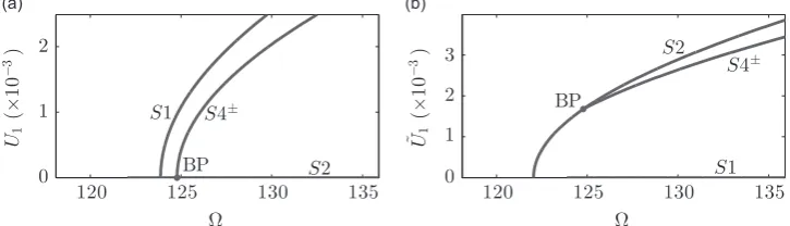
~na,S47 describes responses in whichUa¼U~aand the bifurcation occurs at zero-amplitude.

As an example, we now consider a cable with a length of 1.5 m, a diameter of 5 mm, a density of 3000 kg m3_{, Young's}

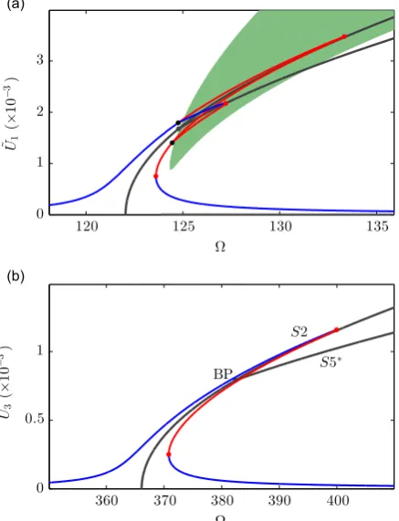
Modulus of 21011Pa and a static tension of 200 N, as originally described in[12].Fig. 2shows the backbone curves for the case wherea¼b¼1 for theﬁrst in- and out-of-plane modes. The non-zeroS1 andS2 solutions are conﬁned toU1, panel (a),

andU~1, panel (b), respectively. At approximately

Ω

¼124:8 rad s1, the mixed-mode backboneS47 bifurcates off theS2 solution branch withU1¼0, with increasingU1andU~1away from the bifurcation point.

3.2. The phase-unlocked case: aab

Considering the general case wherea_ab, Eqs.(13)and(14), we again have the two single-mode solutionsS1 andS2 (Eqs.

(17)and(18)). In addition, as witha¼b, it is possible to have solutions where both modes are present. Taking Eqs.(13)and

(14)and eliminating

Ω

¼

_ω

rk=kgive

2

ra¼

ω

~

2

nbþ

ν

11b2

4m 2a

2_U2

aþ3b

2_~ U2b

~

U2b¼

a2 b2U

2

aþ 4m a2_b2

_ν

11

ω

2

na

a2 b2

ω

~

2

nb

: (24)

Note that there is no phase condition imposed on the modal contributions, this is indicated by thesuperscript. HereUa¼0 is a valid solution and at this point the solution lies onS2, hence this solution branch bifurcates fromS2.

Fig. 3shows the case wherea¼1 andb¼3, in the projection of the response frequency,

Ω

, against the fundamental response amplitude of the third out-of-plane mode,U~3. It can be seen that it is qualitatively similar to the plot shown in

[image:6.544.93.456.557.661.2]

(7)

panel (b) ofFig. 2, although it should be noted that on theS5branch the corresponding response in theﬁrst in-plane mode, with response amplitudeU1, will be at one-third the frequency of theU~3component. We note that, to get a full picture of the dynamic interactions in the cable, all combinations of modes must be considered; however here we show an example interaction between a pair of modes.

4. Internal resonance

Now we consider the potential for the system to exhibit internal resonance, i.e. to respond in a mode that is not directly excited. This will be achieved by considering the amplitude response stability of an unforced mode. If the zero-amplitude response solution is unstable, due to the presence of another mode, then an internal resonance of the unforced mode will be observed. Theﬁndings will be applied to our example system by considering the response of theath in-plane

mode when the cable is excited out-of-plane close to the frequency of thebth out-of-plane mode. From the backbone

analysis, it is revealed that the two-mode cable system is likely to exhibit internal resonance due to the presence of mixed-mode backbone curves. This potential internal resonance is examined by considering the stability of the zero-amplitude response solution to theath in-plane mode.

To assess the stability of the zero-solution of an unforced mode in a general system, we must consider the response of the mode when subjected to a perturbation away from zero. This is achieved by allowing the amplitude and phase of the response to vary slowly in time which, for thekth mode, may be expressed using

uk¼upkþumk¼

Upkð Þ

ε

t

2 e

jωrktþUmkð Þ

ε

t

2 e

jωrkt; ₍₂₅₎

where, from comparison with Eq.(2),Upk¼UkejϕkandUmk¼Ukejϕk. Here we have two time-scales: the oscillatory motion at frequency

ω

rk, and a slowly varying amplitude represented by the amplitude dependence on

ε

twhere

2

rk

2 Upkþj

ω

rkU_pk

!

ejωrkt; _u€

mk¼

ω

2

rk

2 Umkj

ω

rkU_mk

!

ejωrkt: ₍₂₆₎

Here the ﬁrst derivatives are expressed to order

ε

0_{as they will only be used in small terms in the equations of motion}

(damping is assumed to be small), whereas the second derivatives are expressed to order

ε

1_{as they will be used in large}

terms, hence preserving the accuracy of the solution to order

ε

1_.

To proceed, this solution is substituted into the resonant equation of motion for an unforced mode

€

ω

2

nk

ω

2rk

Upkþ2NukþðuÞ

2

_ζ

k

ω

nk

ω

rkUpk

;

_

Umk¼ 1 2

ω

rk

j

ω

2

nk

ω

2rk

Umkþ2NukðuÞ

2

_ζ

k

ω

nk

ω

rkUmk

[image:7.544.163.380.55.198.2]

: (27)

(8)

Expressing this in the formz_¼fðz;tÞwherez¼ fUpk UmkgT, steady-state solutions,zs, may be found by solvingfðzs;tÞ ¼0. The stability of these steady-state solutions may be assessed, to theﬁrst order of accuracy of a Taylor series expansion, by examining the eigenvalues ofDfzðzs;tÞ, whereDfzðz;tÞis the Jacobian offðz;tÞ; if the real part of the eigenvalues are positive then the solution is unstable, see for example[4]. Using Eq.(27), the Jacobian may be expressed as

Dfzðz;tÞ ¼ 1 2

ω

rk

j

ω

2

nk

ω

2rkþ2∂N

þ

uk=∂Upk

; (28)

where we have used Eq.(10)to reﬂect that fact thatNukðuÞhas ejωrktand ejωrktterms. Since we are interested in the zero-amplitude response solution, we need to setz¼zs¼ ½0 0T. Additionally, it can be assumed that the perturbed solution is small, and hence any terms containingUi

pkU j

mkwhereiþj41 are considered to be negligible.

4.1. The form of the resonant nonlinearities

Before proceeding, it is worth considering further the form ofNukðuÞ. Firstly, we know that all terms contain at least one

Upk1 orUmk1 term, otherwise the zero-amplitude response solution would not exist. Secondly, we know that these terms are resonant, but, considering Eq.(A.1), we can see that there are two ways of satisfying this: either via a positive or a negative root. We also know that the higher order terms of½Upk; Umkdo not need to be considered in the stability assessment as they disappear when evaluating the Jacobian forz¼zs¼ ½0 0T. Finally, we know thatNukðuÞis real.

Considering a multimode system with the zero-amplitude response solution in modek, which has resonant frequency

ω

rk¼rk

Ω

, there are four possible types of resonant term which are functions of eitherUpk 1

orUmk 1

, these are

p1: upk ∏ i;iak

uspi

piu smi

mi with:

X

i;iak

riðspismiÞ ¼0; (29)

p2: upk ∏ i;iak

uspi

piu smi

mi with:

X

i;iak

riðspismiÞ ¼ 2rk; (30)

p3: umk∏ i;iak

uspi

piu smi

mi with:

X

i;iak

riðspismiÞ ¼2rk; (31)

p4: umk ∏ i;iak

uspi

piu smi

mi with:

X

i;iak

riðspismiÞ ¼0: (32)

Possibilitiesp1 andp4 place no condition on the response frequency

ω

rkand hence are phase-unlocked terms with respect

to the kth mode. They also result in a positive and negative complex exponential in time for the upk and umk terms

respectively, and so appear in the leading-diagonal terms of the Jacobian. Furthermore, as these terms may be writtenNuukuk, whereNuku is time-independent, it may be seen thatNuku must be real. In contrast,p2 andp3 require a frequency relationship between the kth mode and the other modes in the system. Using Eq.(2), this results in a phase of the nonlinear term, relative to the linear term, of2

_ϕ

kþ

P

i;iak½

ϕ

iðspismiÞ ¼n

π

for both solutions. Asp2 is a negative complex exponential in time andp3 a positive one, these phase-locked terms will appear in the off-diagonals of the Jacobian, and these terms form a complex conjugate pair, ensuring thatNukðuÞis real.

Using the response solution given by Eq.(25), this allows us to write

NukðuÞ ¼NuukUpkejωrktþNuukUmkejωrktþNlukUpkejωrktþN l

ukUmkejωrktþh:o:t ., (33) where superscriptsuandlindicate phase-unlocked and locked terms respectively, and the overbar indicates the complex conjugate, and we note thatNuukis real. Additionally, note that these terms are in the orderp1,p4,p2 andp3.

Using this, the form of the resonant nonlinearities allows the Jacobian matrix, Eq.(28), to be rewritten as

Dfzðz;tÞ ¼ 1 2

ω

rk

j

ω

2

nk

ω

2rkþ2N u uk

2

_ζ

k

ω

nk

ω

rk j2Nluk j2Nl_uk j

ω

2

nk

ω

2rkþ2N u uk

₂

_ζ

k

ω

nk

ω

rk

0 @

1

2

k

ω

ω

4mU~pbU~mb; N

2aa 16m2U~

4

a; (38)

where we have noted thatU~paU~ma¼U~

2

aby comparing Eqs.(2)and(25).

Note that in the cable analysis we could have considered the forcing of many out-of-plane modes. This would have shown that theith in-plane modes can only be triggered, but will not necessarily be triggered, by a response in theith out-of-plane mode as it is just this mode which provides a phase-locked coupling. It is also interesting to note that there are no phase-locked terms between different in-plane or between different out-of-plane modes (the equations take the same form as between an in- and an out-of-plane mode). A special case is when the cable is inclined, when additional parametric forcing terms are introduced due to the inclination, allowing a 1:2 resonance, see for example[17,18].

Fig. 4(a) shows the forced response of the cable due to out-of-plane support excitation when theﬁrst in-plane and the

ﬁrst out-of-plane modes are considered. For this, and subsequent ﬁgures, the forced response was calculated using

numerical continuation, whereas the backbone curves were generated from the analytical solutions derived earlier. Note that forced responses may also be found analytically using the second-order normal form technique_–see, for example,

[5,14]. Here, however, numerical continuation is employed to validate the assumptions used toﬁnd the backbone curves. The transitions between the white and the green background toFig. 4(a) mark the resonant tongue, given by Eq.(38). The points at which the primary forced response curve, containing only the out-of-plane mode, meets this boundary, coincide with bifurcation points. An additional branch, containing both the in- and out-of-plane modes, emerges from these bifur-cation points and envelops theS47 backbone. In the case of the upper bifurcation point, it can be seen that the solution followingS2 becomes unstable at the bifurcation, indicating the loss of stability of the zero-amplitude response solution of the in-plane mode. In contrast, for the case where theﬁrst in-plane and the third out-of-plane modes are considered,Fig. 4

(b), there is no resonant tongue, and the response envelopsS2 throughout.

5. Stiffening effects

We have seen that, to observe internal resonance between a forced and an unforced mode, phase-locking resonant terms are necessary but not sufﬁcient. In the case of the cable example such terms only exist between thekth in- andkth

out-of-plane modes. The resulting motion envelops a mixed-mode backbone curve (or NNM branch), namely theS47 solution

branch for the cable example. We now consider the effect of other modes on the onset of internal resonance between a forced and an unforced mode that have phase-locking resonant terms. For this discussion we consider the cable example and, speciﬁcally, we investigate the inﬂuence of an additional out-of-plane mode that is subjected to near-resonant forcing.

The cth out-of-plane mode may experience near-resonant excitation when the support motion is

vℓ¼Vbcosðb

Ω

tÞþVccosðc

Ω

tÞ. From Eq.(4), this leads to the modal equations of motion, written

mq€aþ2

ζ

a

ω

naq_aþ

ω

2naqa

_þ

_ν

aaq3aþ

ν

abqaq~

2

bþ

ν

acqaq~

2

cþ3

γ

aaq2aþ

γ

baq~

2

bþ

γ

caq~

tÞ;

(39)

whereRij¼ m2ð 1Þ

i

iπ j

2

Vj, and where, from Eq.(4),qa¼za,q~b¼ybandq~c¼yc.

(10)

out-of-plane response terms are large compared to the forcing terms and soecan be neglected when compared tov. This allows us toﬁnd, albeit approximate, solutions using the analysis outlined in the previous sections.

Using this approximation, we now consider how the presence of the cth out-of-plane mode inﬂuences the modal

interactions between theath in-plane andbth out-of-plane modes (wherea¼b). The analysis used to identify the NNMs relating to theath in-plane andbth out-of-plane modes is modiﬁed to include terms due to the presence of the directly excitedcth out-of-plane mode, due to the

ν

acqaq~

2

c and

ν

bcq~bq~

2

c terms in the equations of motion. Redeﬁning the resonant response vector asu¼ ½uau~bu~c>¼ ½uau~au~c>, the vector containing the resonant nonlinear terms for the three modes, formerly Eq.(8), is given by

Nuð Þ ¼u 1

cau~pau~mau~cþ3

ν

ccu~pcu~mcu~c

0 B B B @

1 C C C

A: (40)

Here we have made use of the fact that we are interested in the case wherea¼b(and soaac).

Considering the unforced systemu€þ

_Λ

uþNuðuÞ ¼0, theS2 (i.e.ath out-of-plane-only response) andS47 (i.e.ath in-plane andath out-of-plane phase-locked response) now have the additional condition thatU~c¼0. However, if thecth mode exhibits a response, the backbone curves are affected due to the action of the last term in each of theﬁrst two rows ofNu. The phase-locked, free response equations, Eqs.(15)and(16), are now

ω

2

naa2

Ω

2_þ

ν

aa 4m 3U

2

aþð2þpÞU~

2

aþ2U~

2

c

h i

n o

Ua¼0; (41)

~

ω

2

naa2

Ω

2_þ

ν

aa 4m ð2þpÞU

2

aþ3U~

2

aþ2U~

2

c

h i

n o

~

Ua¼0: (42)

[image:10.544.167.386.58.344.2]

Hence the response solution is modiﬁed away from the backbone expression forS2 due to the presence of theU~ca0

Fig. 4.Forced response of the cable using a two-mode model consisting of theath in-plane mode and thebth out-of-plane mode, where (a)a¼b¼1 and (b)a¼1 andb¼3. Backbone curves are shown in dark grey, stable and unstable forced responses are shown in blue and red respectively and the loss of stability of the zero-amplitude response solution for the in-plane mode is shown as a transition between the white and the green backgrounds. These backbone curves correspond to those shown in Figs. 2 and 3, and are computed using the parameters m¼0:04418 kg, ωn1¼122:04 rad s1,

~

(11)

response resulting in

Ua¼0; a2

Ω

2¼

ω

~2naþ

ν

ac 2mU~

2

c

þ3

ν

aa 4mU~

2

a: (43)

Likewise,S4_a7¼bbecomes

a2

Ω

2¼

ν

aa 2m U~

2

aþU

2

a

þ

ν

ac 2mU~

2

c

þ1

2

ω

2

naþ

ω

~

2

na

; (44)

~

U2a¼U

2

aþ 2m

ν

aa

ω

2

na

ω

~

2

na

: (45)

It can be seen that the effect of theU~cresponse is to shift the solutions in the frequency plane. Note that these solutions are not necessarily backbones capturing a NNM response of the system, as NNMs require a periodic motion, whereas here the frequency of thecth out-of-plane mode is unconstrained, i.e. it is not necessary that

ω

~rc¼c

Ω

. However they do demon-strate that the presence of other modes makes the system appear stiffer. Physically, this can be interpreted as a change in the tension of the cable, due to the presence of other modes–the dynamic tension of a cable contains zero-frequency response terms of the form

θ

2kUk, where

θ

kis the modeshape of thekth mode[4]. Related to this, theﬁnal example in[14]shows that, when excited out-of-plane, the zero-frequency cable response in all the in-plane modes is equivalent to a correction to the static sag. It can be shown that the forced response of theath out-of-plane mode is similarly affected, namely the cable appears stiffer.

We now consider the effect of thecth out-of-plane mode on the resonant tongue, recalling that this marks the onset of a response in theath in-plane mode, triggered via the correspondingath out-of-plane mode, due to phase-locking terms between these modes. Due to the additional nonlinear terms for theath in-plane mode, due to thecth out-of-plane mode, see Eq.(40), theNuuaterm, see Eq.(33), is modiﬁed to

Nu ua¼

ν

aa

4mU~paU~maþ

ν

ac

4mU~pcU~mc: (46)

Using Eq.(36), the stability condition, for the case where there is a constantU~cresponse, may be written as

ac 2mU~

2

c

2

¼

ν

2aa 16m2U~

4

a: (47)

As with the solution curves, the effect of a non-zeroU~ccan be viewed as a shift in the frequency domain, equivalent to having an adjusted natural frequency,

ω

^na, of the form

^

ω

2

na¼

ω

2naþ

ν

ac 2mU~

2

c: (48)

This adjustment to the effective linear natural frequency is identical to the adjustment for the solution curves.

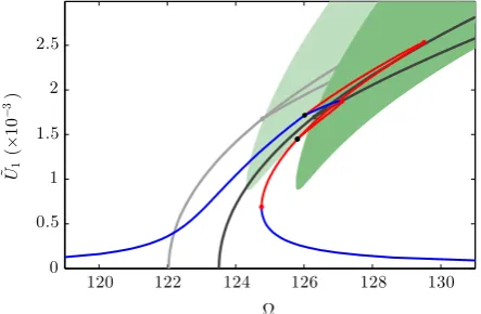
[image:11.544.160.382.507.652.2]

Considering the cable system used in the previousfigures, we can view the effect of thecth out-of-plane mode. Firstly we explore the somewhat artificial example where the forcing is such that the resonant response amplitude of thecth out-of-plane mode,U~c, is constant and the harmonics are assumed to be small.Fig. 5considers the case wherea¼b¼1 andc¼3, and shows the response of the cable in terms of the resonant amplitude of theath, i.e.first out-of-plane mode. The single-mode response to the forcing is shown, along with the bifurcation points at which the mixed-single-mode response is triggered (black dots) and the subsequent mixed-mode response. To aid comparison with the case where the resonant response amplitude of the third out-of-plane mode,U~3, is zero, the backbone curves and resonant tongue for theU~3¼0 case,Fig. 4

(12)

(a), are shown in light grey and green respectively. It can be seen that the resonant tongue and unforced-undamped responses are both shifted in frequency due to the presence of the third out-of-plane mode. Likewise, the forced response is shifted, but here we note that the peak amplitude of the response is also affected due to the increased frequency at which the peak response occurs (this can be seen when compared withFig. 4(a)).

These responses can be represented on a 3D plot, seeFig. 6. Here the backbone curve (whereU~3¼0) has been projected onto the unforced, undamped system response surface (shaded in blue) and the resonant tongue onto a resonant tongue surface (shaded in green). The two forced responses (corresponding toFigs. 4(a) and5) are also shown for the case where there is no in-plane response, and where black dots indicate the points at which the in-plane response is triggered.

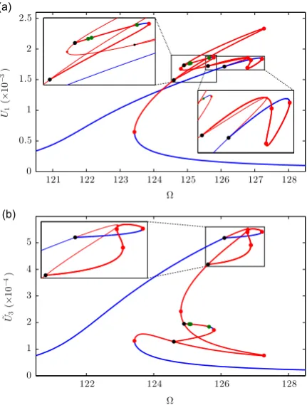
Now, considering the more realistic case in which the third out-of-plane mode is excited at a constant amplitude of support motion, due to the interactions between the two out-of-plane modes the stiffening effect varies with excitation frequency.Fig. 7shows the response for the case where the in-plane resonant motion is zero, along with the internally resonant branches. It can be seen that the resonant tongue, which shifts asU~3increases, due to the stiffening effect, captures these trigger points well.

[image:12.544.151.399.58.220.2]

This discussion indicates that, when multiple out-of-plane modes are present, while the in-plane mode is only triggered by the corresponding out-of-plane mode, i.e. whena¼b, the presence of other out-of-plane modes will alter the behaviour

Fig. 6.Forced response of the cable using a three-mode model consisting of thefirst in-plane mode, thefirst and third out-of-plane modes, showing the plane of unforced undamped responses and the resonant tongue. This represents the artificial case where the resonant response amplitude of the third out-of-plane mode, U~3, is constant. These responses have been computed using the same parameters as those used in Fig. 5; i.e.m¼0:04418 kg, ωn1¼122:04 rad s1, ω~n1¼123:9 rad s1, ν11¼1:417107kg m2s2, γ11¼1:188104kg m1s2, γ31¼1:069105kg m1s2, ζ1¼ζ~1¼0:002 andV¼0:015 mm. (For interpretation of the references to colour in thisfigure caption, the reader is referred to the web version of this paper.)

[image:12.544.150.401.289.452.2]

(13)

of this interaction. Therefore, these non-resonant out-of-plane modes must be considered in order to accurately predict the dynamic behaviour, and the points at which an internal resonance is triggered.

6. Conclusions

In this paper, the phenomenon of phase-locking between modes, and its inﬂuence on internal resonance has been

considered in detail. In particular, using the example of a taut cable, expressions for both phase-locked and phase-unlocked backbone curves were developed. This analysis was initially based on two modes–one in-plane and one out-of-plane. From this it was shown that phase-locking may only occur between corresponding modes, i.e. theath in-plane andath out-of-plane, while two non-corresponding modes do not exhibit phase-locking. Both the phase-locked and the phase-unlocked cases lead to mixed-mode backbone curves that bifurcate from single-mode backbone curves. However, these mixed-mode backbone curves are distinct as, notably, no speciﬁc condition between the linear modes is present for the phase-unlocked case.

Taking a general, two-mode, weakly nonlinear system, a stability analysis was used to show that phase-locking is necessary for an internal resonance to occur. Considering the out-of-plane forced responses of the cable, it was shown that the mixed-mode, locked backbone curves correspond to internally resonant interactions, whereas the phase-unlocked backbone curves do not. This stability analysis was also applied to the cable system to demonstrate that the resonant tongue, described using the analysis, could accurately predict the onset of internal resonance.

[image:13.544.163.379.55.340.2]

As phase-unlocked interactions do not lead to internal resonance, it might, atfirst, appear that they are of little interest in the analysis of nonlinear behaviours. However, in thefinal section of this paper, it was demonstrated that the presence of phase-unlocked modes may lead tostiffeningeffects in the system. These were shown to influence the internally resonant responses observed between other, phase-locked, modes. This was demonstrated by extending the two-mode model of the cable, where corresponding in- and out-of-plane modes exhibit phase-locked responses, to include a third, phase-unlocked, out-of-plane mode. The stiffening effect of this third, phase-unlocked mode was shown to cause an apparent shift in the response frequency of the interactions between the other modes.

Fig. 8. Two projections fromFig. 7, showing the forced response of the cable using a three-mode model consisting of theﬁrst in-plane mode, theﬁrst and third out-of-plane modes, for the case whereV3is constant. (a) showsU~1vsΩ, and (b) showsU~3vsΩ. Blue curves denote stable periodic solutions and red curves, unstable periodic solutions. Black dots indicate the intersection with the resonant tongue surface (not shown), and the bifurcations onto the internally resonant responses. The boxes show the internally resonant regions in detail. As inFig. 7, the parameters used here are:m¼0:04418 kg,ωn1¼122:04 rad s1,

~

(14)

For the somewhat artiﬁcial case where the fundamental response of the third mode was held at a constant amplitude, this frequency shift was demonstrated to be constant. The more realistic case, where the response of the third mode varies under forcing, was then shown to exhibit more complex behaviours. However, these behaviours were accurately predicted by the analytical descriptions of the unforced, undamped equivalent responses, and the onset of internal resonance was predicted using the resonant tongues. This demonstrated that, while the phase-unlocked modes do not lead to internal resonance, they can alter the nature of the internal resonance between phase-locked modes.

Acknowledgements

The authors would like to acknowledge the support from the Engineering and Physical Sciences Research Council. S.A.N. and T.L.H. are supported by EP/K005375/1 and D.J.W. is supported by EP/K003836/1.

The data presented in this work are openly available from the University of Bristol repository athttp://dx.doi.org/10. 5523/bris.1veiinwd99sbw1rko1sp034qv4.

Appendix A. Normal form transformation

In this work we use the second order normal form technique, originally developed by[5], to apply a nonlinear transform to Eq.(1)that removes harmonic terms leaving just the resonant terms–writtenhandurespectively. Note thatsecond orderrefers to the order of the differential equations, in this normal form approach the usual transformation to state-space coordinates (see for example [21,19]) is avoided, instead the transforms are applied directly to the oscillator equations resulting in more compact expressions [15,4]. Considering the transformation of the modal equation of motion to the resonant equation of motion, Eq.(3), with the restrictions that the damping is modal and the forcing in any mode is near-resonant. The derivation toﬁndNuandhðuÞinvolves Taylor series expansions allowing the degree of accuracy (and resulting complexity) to be selected. Discussions on accuracy are given in [5,20]. Adopting theﬁrst degree of accuracy gives the approximation NðuþhðuÞÞ NðuÞ ¼Nðup;umÞ where the transformed coordinates have been split using u¼upþum, resulting in a trial solution of the form given in Eq.(2). By writingNðup;umÞ ¼nuallowsNto be separated into the vector

u, which is of lengthLand contains all the combinations ofupiandumi, and the matrixn, containing the corresponding coefﬁcients. The transform and transformed nonlinear terms may then be written ashðup;umÞ huandNuðup;umÞ nuu, where the approximations indicate that higher-order Taylor series terms have been neglected. For theith mode (ofN) and theℓth element inuthe relationship betweenn,handnuis given by

ni;ℓ¼nu;i;ℓþ

β

i;ℓh

i;ℓ with:

β

i;ℓ¼

XN

n¼1

ðspnℓsmnℓÞ

ω

rn

!2

_ω

2

ri; (A.1)

wheres is deﬁned via the general form for theℓth element inu,

u_ℓ¼ ∏N n¼1

uspnℓ

pnusmnmnℓ

: (A.2)

When

β

i;ℓ¼0, the term is resonant and we setni;ℓ¼nu;i;ℓ, otherwise the term is placed in the transform usinghi;ℓ¼ni;ℓ=

β

i;ℓ. Note that we generate matrix

β

with the½i;ℓth element being

_β

i;ℓhowever this cannot be used in matrix multiplications as the relationship withnis indicial. See, for example,[5,15,4]for a derivation of the expressions presented above. These references also deal with the case where the forcing is non-resonant and the damping is not necessarily resonant.

References

[1]J. Guckenheimer, P. Holmes,Nonlinear Oscillations, Dynamical Systems, and Bifurcations of Vector Fields, Springer-Verlag, New York, 1983. [2]M. Cartmell,Introduction to Linear, Parametric and Nonlinear Vibrations, Chapman and Hall, London, UK, 1990.

[3]A. Nayfeh, P. Pai,Linear and Nonlinear Structural Mechanics, Wiley, Weinheim, Germany, 2004.

[4]D.J. Wagg, S.A. Neild,Nonlinear Vibration with Control, second edition, Springer-Verlag, Berlin, Germany, 2014.

[5] S.A. Neild, D.J. Wagg, Applying the method of normal forms to second-order nonlinear vibration problems,Proceedings of the Royal Society, Part A: Mathematical, Physical and Engineering Science467(28) (2011) 1141–1163.

[6]A.F. Vakakis, L.I. Manevitch, Y.V. Mikhlin, V.N. Pilipchuk, A.A. Zevin,Normal Modes and Localization in Nonlinear Systems, Wiley, New York, 1996. [7]A.F. Vakakis, R.H. Rand, Normal modes and global dynamics of a two-degree-of-freedom non-linear system–I. Low energy,International Journal of

Non-linear Mechanics27 (5) (1992) 861–874.

[8]G. Kerschen, M. Peeters, J.C. Golinval, A.F. Vakakis, Nonlinear normal modes, Part I:a useful framework for the structural dynamicist,Mechanical Systems and Signal Processing23 (Sp. Iss. (SI) 1) (2009) 170–194.

[9]R. Lewandowski, Solutions with bifurcation points for free vibration of beams:an analytical approach,Journal of Sound and Vibration177 (1994) 239–249.

[10]R. Lewandowski, On beams, membranes and plates backbone curves in a cases of internal resonance,Meccanica31 (1996) 323–346.

(15)

[12] T.L. Hill, A. Cammarano, S.A. Neild, D.J. Wagg, Out-of-unison resonance in weakly-nonlinear coupled oscillators,Proceedings of the Royal society, Part A: Mathematical, Physical and Engineering Science471 (2015) paper 20140332.

[13]T.L. Hill, A. Cammarano, S.A. Neild, D.J. Wagg, Interpreting the forced responses of a two-degree-of-freedom nonlinear oscillator using backbone curves,Journal of Sound and Vibration349 (2015) 276–288.

[14]S.A. Neild, A.R. Champneys, D.J. Wagg, T.L. Hill, A. Cammarano, The use of normal forms for nonlinear dynamical systems,Philosophical Transactions of the Royal Society, Part A: Mathematical, Physical and Engineering Science373 (2015). paper 20140404.

[15] S.A. Neild, Approximate methods for analysing nonlinear structures, in: L.N. Virgin, D.J. Wagg (Eds.)Exploiting Nonlinear Behaviour in Structural Dynamics, Springer-Verlag, Berlin, Germany, 2012.

[16]P. Warnitchai, Y. Fujino, T. Susumpow, A non-linear dynamic model for cables and its application to a cable-structure system,Journal of Sound and Vibration187 (1995) 695–712.

[17] A. Gonzalez-Buelga, S.A. Neild, D.J. Wagg, J.H.G. Macdonald, Modal stability of inclined cables subjected to vertical support excitation,Journal of Sound and Vibration318 (3) (2008) 565–579.

[18]J.H.G. Macdonald, M.S. Dietz, S.A. Neild, A. Gonzalez-Buelga, A.J. Crewe, D.J. Wagg, Generalised modal stability of inclined cables subjected to support excitations,Journal of Sound and Vibration329 (21) (2010) 4515–4533.

[19]A.H. Nayfeh,Method of Normal Forms, Wiley, Weinheim, Germany, 1993.

[20] S.A. Neild, D.J. Wagg, A generalized frequency detuning method for multidegree-of-freedom oscillators with nonlinear stiffness,Nonlinear Dynamics 73 (2013) 649–663.