Modeling the dispersion of drilling muds using the bblt model: the effects of settling velocity

Modeling the dispersion of drilling muds using the bblt model: the

effects of settling velocity

Haibo Niu

Adam Drozdowski

, Tahir Husain

, Brian Veitch

,

Neil Bose

, and Kenneth Lee

a

Memorial University of Newfoundland, St. John’s, NL, Canada, A1B 3X5 b

Bedford Institute of Oceanography, Dartmouth, NS, Canada, B2Y 4A2

c

Australian Maritime College, Launceston, Tasmania, Australia, 7250

Key Words: drilling muds, dispersion, settling velocity, benthic boundary layer model

Abstract

The benthic boundary layer transport (bblt) model was widely used in the Atlantic

Canadian offshore region to assess the potential impact zones from drilling wastes

discharges from offshore oil and gas drilling. The current version of the bblt uses a

single-class settling velocity scenario which may affect its performance, as settling

velocity is size, shape and material dependent. In this study, the effects of settling

velocity on bblt predictions were assessed by replacing this single-class settling velocity

scenario with a multi-class size dependent settling velocity scenario. The new scenario

was used in a hypothetical study to simulate the dispersion of barite and fine-grained

drilling cuttings. The study showed that the effects of settling velocity on bblt predictions

are spatial, temporal, and material dependent.

1. Introduction

The exploration and extraction of offshore oil and gas from beneath the ocean floor

requires the disposal of drilling wastes such as spent drilling muds and rock cuttings. In

disposal of drilling wastes. However, the discharge of drilling wastes into the marine

environment may pose adverse impacts, such as growth inhibition, mortality, and

smothering, of marine organisms (Gordon et al., 2000; Cranford et al., 1999). In order to

give operators and regulatory agencies the ability to assess the fate of drilling wastes

under a variety of ocean conditions, mathematical modeling of the transport processes of

drilling muds become important.

To date, a number of transport models for drilling wastes have been developed. These

include: the Offshore Operators Committee (OOC) model (Brandsma and Saucer, 1983),

bblt model (Drozdowski et al., 2004), NewCut model (Carles, 1996), MUDMAP model

(ASA, 2006), ParTrack model (Rye et al. 2006), and PROTEUS model (Sabeur and

Tyler, 2001). It was shown by a systematic review (Khondaker, 2000) that the ultimate

accuracy of transport models relies on our knowledge of complex transport processes

(such as settling and flocculation) of drilling wastes. This has been proved by the study of

Carles and Bryden (1999) in which they found that the transport models are very

sensitive to the type of settling equations used and therefore to the size and shape of the

drilling cuttings. Khondaker (2000) also concluded there is no single, fully validated and

universal drilling waste transport model, due to the still only partially understood

transport processes.

Over the past two decades, extensive laboratory work has been conducted on the

settling and flocculation processes of drilling wastes (Huang 1992; Chien, 1992; Gerard

1996; Carles, 2000; Curran et al. 2002; Niu et al., 2003) and this makes it possible to

improve the transport models with the latest findings. The benthic boundary layer

process and it has been used widely in the Atlantic Canadian offshore region as part of

the environmental impact assessment for a number of projects (Gordon et al., 2000;

Cranford et al., 2003; Thomson et al., 2000; Hannah et al., 2006; Tedford et al., 2002,

2003). A limitation of these previous studies is that they use of a single class of settling

velocity, rather than multi-class settling velocities that are size and shape dependent.

Therefore, the focus of the present paper is to use the bblt model with an improved

settling velocity scenario to characterize the drift and dispersion of drilling wastes. The

simulation results are compared with previously used settling velocity scenarios to show

the effects of the new simulation strategy.

bblt Model

The bblt was developed by Bedford Institute of Oceanography to predict the transport

and dispersion of particulate drilling wastes in the benthic boundary layer. The model

assumes that all the discharge materials enter the benthic boundary layer and thus neglect

the mechanism of plume surfacing. The primary mechanisms modeled by bblt are the

horizontal dispersion due to the interaction of vertical mixing and vertical shear, mud

flocculation and break-up, drift, and vertical mixing. The latest version, bblt v7.0, also

integrated a biological impact module (Drozdowski et al., 2004).

The bblt is a particle based model which treats the drilling wastes load mass M as N

pseudo-particle packets with mass m=M/N and settling velocity w. The basic output of

the bblt is the time series packet positions, Xn(t), Yn(t), Zn(t). The movement of the

packets has two components: horizontal dispersion and vertical distribution. The

horizontal dispersion of the packets is measured by the horizontal variance of the packets

distribution (m2_{). The effective diffusivity}

K (m2/s) is defined as (Csanady 1973)

2

t K ∂ ∂ = 2 2 1

σ

where the overbar denotes a time averaging. In two dimensions, the variances, and

, along the major and minor axes of the horizontal projection of the distribution are

calculated. The effective diffusivity for this case is defined as

2 max σ 2 min

σ

D= (2)

where Kmax and Kmin are the effective horizontal diffusivities along the major and minor

axes, respectively. The Kmax and Kmin are defined by equation (1).

The vertical distribution of the packets is parameterized by a sediment concentration

Rouse profile c(z) as

⎪⎩ ⎪ ⎨ ⎧ > ≤ = δ δ δ

δ z z

c z z a c z c p p a ) / ( ) / ( ) ( 2 1 (3)

where z is the vertical coordinates, a is the sediment reference height below which the

particle motion is negligible, ca is the reference concentration c(a) at height a,

δ

height of the current-wave boundary layer, c_δ is the reference concentration c(δ)at

height

δ

* u w p

κ

= (4)

where the κ is the von Karman constant κ=0.4, w is the settling velocity, u_* =

τ

ρ

is the friction velocity,

τ

water.

The settling velocity in the current bblt can be either fixed (typically 0.5 cm/s or 0.1

cm/s) or stress dependent. The stress dependent settling velocity (as shown in Fig. 1)

considers the flocculation effect by using a three-point velocity. It is assumed that the

velocity w0 (typically 0.5 cm/s). The flocs will remain at this velocity until the friction

velocity exceeds the critical value , at which point the flocs break up into their

individual components and settle at a very low velocity w2 (typically 0.01cm/s). When

the velocity falls below the critical value again, the drilling wastes will be

incorporated into the background marine flocs and settle at a speed of w1 (typically 0.1

cm/s). Thereafter, the settling velocity will be either w1 or w2 depend on the value of

(Drozdowski et al., 2004).

*

u c

u_*

*

u c

u_*

*

u

The bblt calculates the concentration (mass per unit volume) by counting the packets

in a user specified volume, for example a cylinder of radius r, from z1 to z2. The bblt also

allows the user to use a user defined rectangular grid to calculate the concentration.

Simulation Strategy

As the settling velocity equation used is very important for the accuracy of a drilling

waste transport model (Carles and Bryden, 1999), the performance of the bblt is

expected to be improved by replacing the current single-class settling scenario with a

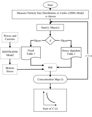
more validated multi-class size dependent scenario. A new simulation strategy is

proposed in this paper as illustrated in Fig 2.

The first part of the new simulation strategy is characterizing the drilling wastes. This

becomes essential because the settling velocity of drilling wastes depends on the particle

size, shape, and type of drilling fluids used.

The discharge generally comprises drilling muds (or fluids) and drilling cuttings. The

drilling fluids are a suspension of solids (mainly barite and bentonite) and dissolved

discharging varies from country to country and from case to case, most regulations permit

four types of discharges: water-based muds (WBM); cuttings produced by using water

based muds (WBC); synthetic-based muds (SBM); and cuttings produced by using

synthetic based muds (SBC). The later two are only permitted in certain conditions. The

particles modeled by the bblt were forced to agree with the Rouse vertical profile, thus a

coarse particle with large settling velocity will hardly be moved by the bottom stress.

Therefore, the bblt should only be used for WBM, SBM and the fine-grained portion of

WBC and SBC. The cut-off size for WBC and SBC is case dependent. In this study, only

the cutting particles with settling velocities less than 1.5 cm/s are considered; this

corresponds to about 70 percent of the total cutting mass according to the data of Rye et

al. (2006).

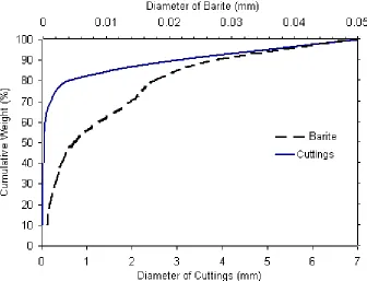
Once the material is identified, information about the particle size distribution of the

material is needed. This can be obtained either from measurements or from a database.

An example of the measured particle size distribution for both drilling cuttings and barite

is given in Fig 3. If the particle size distribution data is unavailable, a database software

(Carles 2000) may be used to generate a distribution according to the drilling conditions

(for example the size of well, depth of well, type of drill-bit, type of drilling muds used

etc.). The whole discharge material can then be divided into n classes of particles with

diameter di and weight Wi(i=1, n).

According to the material, and particle size distribution, different settling velocity

equations (as shown in Table 1) will be used for each of the n particle classes.

The WBC and WBM (mainly barite) both have a particle structure. Once discharged,

descend independently at the early stage. The settling velocity correlation from Chien

(1994) can be used for the individual particles. The equation is given in Equation 5:

⎥ ⎥ ⎦ ⎤ ⎢ ⎢ ⎣ ⎡ − ⎟⎟ ⎠ ⎞ ⎜⎜ ⎝ ⎛ ⎟ ⎟ ⎠ ⎞ ⎜ ⎜ ⎝ ⎛ − +

=_{0.0002403 1 920790.49} − _{1 1}

2 030 . 5 03 . 5 e f f p f e d d e d e w

μ

ρ

ρ

ρ

ρ

μ

where ψ a sphericity factor,

μ

diameter of the particle, ρp is the density of the particle, andρf is the density of the

ambient water.The coarse particles tend to settle rapidly around the discharge point while

the fine particles gradually start to collide together and form flocs which have faster

settling velocities than their originally individual constituent particles. The laboratory

equations developed by Huang (1992) can be used to simulate the settling of flocs, as

shown in Equation (6):

f jd

w= (6)

where j is an empirical constant with values ranging from 12.85 to 23.26, and f is also an

empirical constant with values ranging from 0.52 to 0.59.

The discharged SBC behaves differently than WBC. The synthetic based fluid has low

water solubility and it tends to bind the drilling cuttings and barite together. Therefore,

SBC normally descend fast and will not spread in the water column. The equations by

Niu et al. (2003) can be used to simulate the settling of coarse SBC particles, as shown in

equation (7) d a gd a b b w f f f p

ρ

ρ

ρ

ρ

μ

μ

3 ₊ 2 2 _{+ −} 3

−

= (7)

where a and b are constants dependent on the particle sphericity ψ . Niu et al. (2003) also

32 . 0 84 . 1 07 . 1 4 10 22 .

2 _{x G d}G

w= − (8)

where G is the shear rate or velocity gradient (1/s).

The input of bottom stress can be computed by using the SEDTRAN96 (Li and Amos,

2001) model with measured oceanographic data. The bblt model can then be executed for

each of the n particle classes by using settling velocity equations from Table 1. Total

concentration can be obtained by taking the sum of the n individual concentration

outputs.

Case Study

To test the simulation strategy described above, a hypothetical study was performed

using the data from the North Triumph site south of Sable Island off the south east coast

of Canada. The dispersion of barite near this site has been studied by Hannah et al.

(2003).

Although Carles and Bryden (1996) have concluded the dispersion models are very

sensitive to settling velocity equations, it is still unclear to what degree the bblt will be

affected by it. Therefore, a sensitivity study using only barite and eight different settling

velocities was conducted to show the sensitivity of the bblt to settling velocity equations

before conducting a full analysis using different types of drilling wastes and different

classes of particle sizes.

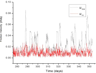
The same discharge rates and the same friction velocity due to current and waves

( ) and due to currents ( ) used by Drozdowski et al. (2004) was used for this study.

The stress is plotted in Fig 4. The period simulated for the sensitivity study was 5 days. cw

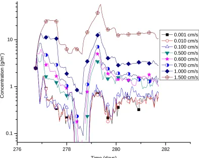
The results of the sensitivity study for this site are shown in Fig 5. It can be seen from

the plot that bblt is very sensitive to the settling velocity. By increase the settling velocity

from 0.1 cm/s to 1.5 cm/s (increased 15 times), the center of mass concentration

(deposited solids in gram per square meter seabed) increased from 0.5 g/m2 to about 20

g/m2 (increased 40 times).

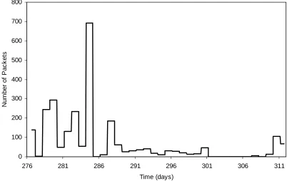
In order to get a result comparable to previous studies, the first set of simulations

considered only the barite from WBM. The time series discharge of barite for this site is

available from Drozdowski et al. (2004) and is presented in Fig 6. According to the

particle size distribution of barite (as shown in Fig. 2), ten particle classes of equal

percentage of weight were used (Table 2). For simulation 1, the total number of packets

was 59935 and the mass associated with one packet was 3.536 kg. Similarly, 59935

packets were used for each of the ten classes of simulation 2 and each packet had a mass

of 0.3536 kg. The total mass discharged for both simulations was the same.

To assign the initial settling velocity w0 for flocs, the size of the flocs is needed. As

the current version of the bblt does not have a flocculation process model, assumptions

must be made for the floc size. According to Huang (1992), the floc size of WBM ranges

from 30 μm to 300 μm. It was assumed in this study that the 30 μm floc was produced by

the 0.7 μm particle and the 300 μm floc was produced by the 50 μm particle. Linear

interpolation was performed to derive floc sizes for other particles between 0.7 μm and

50 μm. The w0 was then computed using Equation (6). The w2 in Table 2 was calculated

using Equation (5). Because of the sphericity (in equation 5) distribution is unavailable, a

mean value of 0.8 was used as suggested by Chien (1994). The w0 for large flocs in Table

has a porous structure which reduces its effective density. The settling velocity value for

background marine flocs w1 is the same as that used by Drozdowski et al. (2004).

The materials considered in the second sets of simulations (No.3 and 4 in Table 3)

were fine-grain drilling cuttings (70% of total cuttings). The densities of the drilling

cuttings are normally smaller than barite and therefore their settling velocities are also

smaller. The information about the amount of discharged drilling cuttings is unavailable

and a cutting to barite ratio of 8:1 was assumed based on Rye et al. (2006). For

simulation 3, the total number of packets was 59935 and the mass associated with one

packet was 19.801 kg. Similarly, 59935 packets were used for each of the seven classes

of simulation 4 and each packet had a mass of about 2.829 kg. The total mass discharged

for both simulations was the same.

Results and Discussions

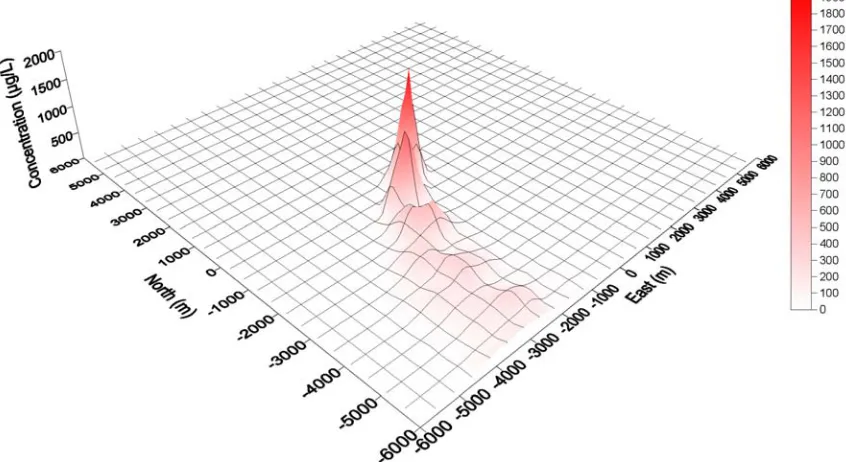
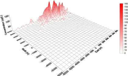
The results for the first set of simulations for barite are shown in Fig. 7 and Fig. 8. Fig.

7 shows the predicted near bottom depth averaged concentration after 120 hours (5 days).

The barite was dispersed to the southwest with a very high concentration near the rig

(East 0 m, North 0 m). Fig. 8 shows the concentration after 900 hours (37.5 days). It can

be seen that the center of mass has moved to the northeast with a very low concentration

near the rig.

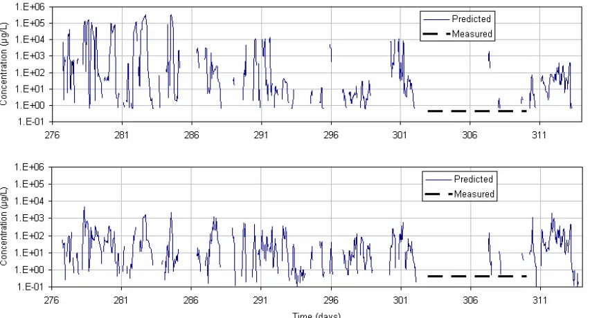
Environmental Effects Monitoring (EEM) data are available for the North Triumph

site. Barite concentration at 38 locations at distances from 250 m to 20 km to the rig were

determined by sampling the bottom sediment and sampling the water and suspended

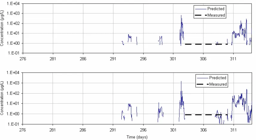
NT-250-7-D3 (250 m southwest) and NT-5000-6-D3 (5000 m southwest) were used to

compare with model predictions. The results are shown in Fig 9 and Fig 10.

It can be seen from the Fig 9 that the new settling velocity strategy does affect the

concentration prediction at early stages of simulation (before day 286) for locations close

to the discharge. The concentration predicted by the multi-class scenario (simulation 2) is

much lower (about two-orders) than the single-class scenario (simulation 1). The reason

is that the new strategy used a set of w0 which are much smaller than the previously used

typical value of 0.5 cm/s. It is also shown by Fig 9 that this effect becomes insignificant

at the later stage of simulation. The concentrations for both simulations are about the

same after day 301. The is because of the initial flocs settling velocity w0 was no longer

in effect after the stress reached the critical value . This can also be seen from Fig. 10

for site NT-5000-6-D3. Overall, although a few sudden variations of concentration have

been predicted over the 7 days EEM period, the majority of the predicted concentrations

are in the same order as the measured values.

cw u_*

The simulation results for fine-grain drilling cuttings are shown in Fig 11 and Fig 12.

For the same location NT-250-7-D3 (see Fig. 11), the simulation 3 is only slightly higher

than simulation 4 at the early stages of discharge (before day 290). The concentrations lie

between 105 _{μg/L and 10}6 _{μg/L. This is different from the barite case in which the}

concentration from the new simulation strategy (No.2) is about two-orders smaller than

the single class simulation (No.1). The predicted later stage concentration for cuttings is

also different from that for barite. The cutting concentration predicted by simulation 4 is

higher than that predicted by simulation 3, while the barite concentration predicted by

although the w0 in simulation 4 is still smaller than that for simulation 3, the high settling

velocity of the coarse particles in cuttings made the difference insignificant. In simulation

3, the cuttings were dispersed away in later stage and resulted in a low concentration as a

smaller w2 were used. On the contrary, the higher w2 for coarse particle in simulation 4

made them less dispersible and resulted in a high concentration.

For location NT-5000-6-D3 (see Fig. 12), because it is far from the rig, the effects of

w0 and w2 become less important. Although the predicted concentrations are still

different, they are of the same magnitude. This does not imply that the choice of settling

velocity is not important for the simulation. This is only because the selected settling

velocity (in Tables 2 and 3) in this study lies within the less sensitive region for bblt

model. Fig 5 shows clearly that the bblt is more sensitive for w greater than 0.1 cm/s and

less sensitive for w smaller than 0.1 cm/s.

Conclusions

The single class settling velocity scenario has been replaced with a multi-class

size-dependent settling velocity scenario. The new scenario was applied in a hypothetical

study to model the dispersion of both barite and fine-grained drilling cuttings. The

simulation showed that the new settling velocity scenario does affect the predicted

concentration.

At locations close to the rig, the new settling velocity scenario predicted a much

smaller barite concentration than the single-class settling scenario at the early stages of

simulation. This is the result of the smaller w0 that were used in the multi-classes

scenario. The predicted concentrations from both scenarios are of same magnitude at the

less than the critical value. Same magnitudes of concentration were also predicted by

both scenarios for locations far from the rig at later stages of simulation (the early stage

concentrations at these locations are zero).

For drilling cuttings, the predicted concentration by the new multi-class scenarios is

only slightly smaller than that predicted by the single-class scenario for locations close to

the rig. This reduced difference between the two scenarios is due to the fast deposition of

relatively coarse drilling cutting particles. Furthermore, the predicted concentration by

the new multi-class scenarios is much higher than that predicted by the single-class

scenario for locations close to the rig. The reason is that the large w2 in the multi-class

scenario makes the coarse particles remain at the site and results in a high concentration

at later stage. On the contrary, the smaller w2 in the single-class scenario makes the

cuttings easily dispersed away and results in a low concentration at later stage.

Similar to the barite, approximately same magnitudes of cutting concentration were

also predicted by both scenarios for locations far from the rig at later stages of simulation.

This does not imply that the choice of settling velocity is not important for these far

locations. This is only because the selected settling velocity (in Tables 2 and 3) in this

study lies within the less sensitive region for the bblt model.

Finally, it should be pointed out that there is still disagreement about w0 amongst

researchers. The values used in this study were based on laboratory measurements

(Huang, 1992, Niu, 2003), which are much smaller than that suggested by Milligan and

Hill (1998). Future research on field observations of w0 is needed to get more accurate

Acknowledgements

The Natural Sciences and Engineering Research Council (NSERC) of Canada and the

Petroleum Research Atlantic Canada (PRAC) provided financial support for this study.

References

Applied Science Associates (ASA). (2006). http://www.appsci.com/mudmap/index.htm.

Brandsma, M. G., Saucer, R. C. (1983). The OOC model: Prediction of short term fate of

drilling fluids in the ocean. Proceedings of Mineral Management Service Workshop

on Discharged Modeling, Santa Barbara, CA, US, February 7-10, 1983.

Carles, L. J. (1996). Simulating the dispersion of offshore drill-cuttings. M.Sc Thesis,

Heriot-Watt University, U.K.

Carles, L. J. (2000). Physical characteristics and aquatic settlement properties of offshore

drill-cuttings. PhD Thesis, Robert Gordon University, Aberdeen, Scotland, U.K.

Carles, L. J., Bryden, I. G. (1999). The sensitivity of a dispersion model to cuttings

settling speeds. Society of Underwater technology Journal, 24, 19-24.

Chien, S-F. 1992. Settling velocity of irregular shaped particles. SPE paper No. 26121.

Cranford, P. J., Gordon, Jr, D. C., Lee, K., Armsworthy, S. L., Tremblay, G. H. (1999).

Chronic toxicity and physical disturbance effects of water and oil-based drilling fluids

and some major constituents on adult sea scallops (placopecten magellanicus). Marine

Environmental Research. 48, 225-256.

Cranford, P.J., Gordon, Jr., D. C., Hannah, C. G., Loder, J. W., Milligan, T. G.,

Muschenheim, D. K., Shen, Y. (2003). Modelling potential effects of petroleum

exploration drilling on northern geoges bank scallop stocks. Ecological Modelling

Csanady, G. T. (1973). Turbulent Diffusion in the Environment. D. Reidel Publishing

Company.

Curran, K., Hill, J. P. S., Milligan, T. G. (2002). The role of particle aggregation in

size-dependent deposition of drill mud. Continental Shelf Research, 22, 405-416.

Drozdowski, A., Hannah, C., Tedford, T. (2004). bblt Version 7 user’s manual. Canadian

Technical Report of Hydrography and Ocean Science, 69 pp.

Gerard, A. L. D. (1996). Laboratory investigations on the fate and Physicochemical

properties of drilling cuttings after discharged into the sea. Physical and Biological

Effects of Processed Oily Drill Cuttings, E&P Forum Report, Paper 3, 16-24.

Gordon, Jr., D. C., Cranford, P.J., Hannah, C.G., Loder, J.W., Milligan, T. G.,

Muschemheim, D. K., Shen, Y. (2000). Modelling the transport and effects on

scallops of water-based drilling mud from potential hydrocarbon exploration on

Geoges Bank. Can. Tech. Rep. Fish. Aquat. Sci. 2317, 115 pp.

Huang, H. (1992). Transport properties of drilling muds and Detroit River sediments.

PhD Thesis. University of Santa Barbara, CA, U.S., May 1992.

Khondaker, A. N. (2000). Modeling the fate of drilling waste in marine environment – an

overview. Computer & Geosciences, 26, 531-540.

Li, M. Z., Amos, C. L. (2001). SEDTRAN96: the upgraded and better calibrated

sediment-transport model for continental shelves. Computers & Geosciences, 27,

619-645.

Milligan, T. G., Hill, P. S. (1998). A laboratory assessment of the relative importance of

turbulence, particle composition, and concentration in limiting maximal floc size and

Niu, H., Husain, T., Veitch, B., Bose, N. (2003). Transport Properties of Offshore

Discharged Synthetic Based Drilling Cuttings, Proceedings of MTS/IEEE Oceans

2003 Conference, Sep 22-26, 2003, San Diego, CA, U.S., Vol 1, 411-416.

Rye, H., Reed, M., Frost, T. K., Utvik, T. I. R. (2006). Comparison of the ParTrack

mud/cuttings release model with field data based on use of synthetic-based drilling

fluids. Environmental Modelling & Software, 21, 190-203.

Sabeur, Z.A., Tyler, A.O. (2001). “Validation of the PROTEUS Model for the Physical

Dispersion, Geochemistry and Biological Impacts of Produced Waters,” In

Proceedings of the 5th International Marine Environmental Modeling Seminar, Oct 9-11, 2001, New Orleans, Louisiana, USA, 209-228.

Tedford, T., Drozdowski, A., Hannah, C. G. (2003). Suspended sediment drift and

dispersion at Hibernia. Can. Tech. Rep. Hydrogr. Ocean Sci. 227, 57 pp.

Tedford, T., Hannah, C. G., Milligan, T. G., Loder, J. W., Muschenheim, D. (2002).

Flocculation and the fate of drill mud discharges. In: SpauldingM. L. (Ed.), Estuarine

and Coastal Modelling: Proceedings of the 7th International Conference. ASCE,

294-309.

Thomson, D. H., Davis, R. A., Belore, R., Gonzalez, E., Christian, J., Moulton, V. D.,

Harris, R. E. (2000). Environmental assessment of exploration drilling on Nova

Scotia. Report prepared for Canada - Nova Scotia Offshore Petroleum Board and

Mobil Oil Canada Properties, Shell Canada Ltd., Imperial Oil Resources Ltd., Gulf

Canada Resources Ltd., Chevron Canada Resources, EnCana Petroleum Ltd., Murphy

Oil Company Ltd., and Norsk Hydro Canada Oil & Gas Inc. Report Prepared by LGL

Hannah, C. G., Drozdowski, A., Loder, J., Muschenheim, K., Milligan, T. (2004). An

assessment model for the fate and environmental effects offshore drilling mud

discharges. Estuarine Coastal and Shelf Science, 70, 577-588.

Start

Measure Particle Size Distribution or Carles (2000) Model

n classes

Size(i), Mass(i)

bblt

d

Fixed

Table 1 Stress depedentTable 1 50μm< <50μm

Concentration Map (i)

i=1,n

Sum ofC(i)

Bottom Stress SEDTRAN96

Model Waves and

Currents

276 278 280 282 0.1

1 10

C

oncentr

a

ti

on (

g

/m

2 )

Time (days)

0.001 cm/s 0.010 cm/s 0.100 cm/s 0.500 cm/s 0.600 cm/s 0.700 cm/s 1.000 cm/s 1.500 cm/s

0 100 200 300 400 500 600 700 800

276 281 286 291 296 301 306 311

Time (days)

N

um

b

er

of

P

ac

k

et

s

Table 1. Settling velocity scenario

Material Sizes Scenario w w0 w2 w1

>50µm F Equation (5) WBF

<50µm S Equation (6) Equation (5) 0.1cm/s

>50µm F Equation (5) WBC

<50µm S Equation (6) Equation (5) 0.1cm/s

>50µm F Equation (7) SBC

<50µm S Equation (8) Equation (5) 0.1 cm/s

* F – Fixed, S – Stress dependent

Table 2 Barite in drilling mud particle diameter, and settling velocity distribution

No Diameter _(μm) Weight _(%) Packets _{Mass (kg)} Packet Floc Size (μm)

w0 (cm/s) w2 (cm/s) w1 (cm/s)

1 Single _Size 100 59935 3.536 Single _Size 5.00E-01 1.00E-02 1.00E-01

2 0.7 10 59935 0.3536 30 1.73E-02 3.89E-05 1.00E-01 1.0 10 59935 0.3536 32 1.79E-02 7.93E-05 1.00E-01 2.0 10 59935 0.3536 37 1.96E-02 3.17E-04 1.00E-01 3.0 10 59935 0.3536 43 2.13E-02 7.14E-04 1.00E-01 9.0 10 59935 0.3536 54 2.44E-02 1.98E-03 1.00E-01 9.0 10 59935 0.3536 75 2.98E-02 6.42E-03 1.00E-01 14.0 10 59935 0.3536 103 3.58E-02 1.55E-02 1.00E-01 18.0 10 59935 0.3536 125 4.01E-02 2.57E-02 1.00E-01 28.0 10 59935 0.3536 180 4.97E-02 6.21E-02 1.00E-01 50.0 10 59935 0.3536 300 6.73E-02 1.98E-01 1.00E-01 Sum 100 3.536

Table 3 Drilling cuttings particle diameter, and settling velocitydistribution

No Diameter _(μm) Weight _(%) Packets _{Mass (kg)} Packet

Floc Size (μm)

w0

(cm/s) (cm/s) w2 (cm/s) w1

3 Single _Size 100 59935 19.8016 Single _Size 5.00E-01 1.00E-02 1.00E-01

4 7 14.28 59935 2.828706 30 1.73E-02 1.69E-03 1.00E-01 15 14.28 59935 2.828706 80 3.08E-02 7.74E-03 1.00E-01 25 14.28 59935 2.828706 143 4.34E-02 2.15E-02 1.00E-01 35 14.29 59935 2.828706 206 5.39E-02 4.21E-02 1.00E-01 50 14.29 59935 2.828706 300 6.73E-02 8.59E-02 1.00E-01

75 14.29 59935 2.829036 1.93E-01

200 14.29 59935 2.829036 1.29E+00