Dynamic response testing method of damage detection in fibre composite structures

(1)

University of Southern Queensland

Faculty of Engineering and Built Environment

DYNAMIC RESPONSE TESTING METHOD OF DAMAGE DETECTION IN FIBRE COMPOSITE STRUCTURES

Dissertation By James Kerr u1004780

Supervised by

Dr Jayantha Epaarachchi

(2)

Abstract

This dissertation analyses the practicality of the use of vibration signatures as a method to monitor structural health of a glass pultrusion square hollow section member and to detect the existence, magnitude and location of damage. 12 nodes spaced evenly along the 1m long beam were the test locations where an accelerometer was placed and an impact hammer was used to cause the forced oscillation. The data was collected using an LMS data acquisition system coupled with the LMS Xpress testware.

Two methods of identifying damage were applied. The empirical mode decomposition and the Hilbert-Huang transformation. The empirical mode decomposition proved inadequate at signifying damage, however, the Hilbert-Huang transformation showed clear indication of damage introduction. Figures of all numerical analysis and results are included. Also pictures to aid in understanding of the experiments are also included. A copy of the entire Matlab code used in the numerical analysis of the oscillatory signal.

Based on the results of the experiments and numerical analysis it is deemed that with further research it may be possible to build a industrially suitable dynamic testing method for a wide variety of complex materials that avoids the requirement of specialised technicians, abundant apparatus, lengthy time and costly processes.

(3)

University of Southern Queensland

Faculty of Health, Engineering and Sciences

ENG4111/ENG4112 Research Project

Limitations of Use

The Council of the University of Southern Queensland, its Faculty of Health, Engineering &

Sciences, and the staff of the University of Southern Queensland, do not accept any

responsibility for the truth, accuracy or completeness of material contained within or associated

with this dissertation.

Persons using all or any part of this material do so at their own risk, and not at the risk of the

Council of the University of Southern Queensland, its Faculty of Health, Engineering &

Sciences or the sta

ﬀ

of the University of Southern Queensland.

(4)

Certification

I certify that the ideas, designs and experimental work, results, analyses and conclusions set

out in this dissertation are entirely my own e

ﬀ

ort, except where otherwise indicated and

acknowledged.

I further certify that the work is original and has not been previously submitted for assessment

in any other course or institution, except where speciﬁcally stated.

(5)

4.3 Experimental Validation ... Error! Bookmark not defined. 4.3.1 Literature ... Error! Bookmark not defined. 4.3.2 Finite Element Analysis ... Error! Bookmark not defined. 4.3.3 LMS Test Ware ... Error! Bookmark not defined. 4.3.4 Supervisory Verification ... Error! Bookmark not defined. Chapter 5| Data Results and Analysis ... 57

5.1 Results from experiment ... Error! Bookmark not defined. Chapter 6| Discussion ... Error! Bookmark not defined. Chapter 7| Conclusion ... 73

References ... 74

Appendices ... 83

Appendix A| Apparatus ... 83

Appendix A1: Fibre-optic Bragg grating sensor ... 106

Appendix A2: Power amplifier ... 106

Appendix A3: Signal generator ... 106

Appendix A4: Solenoidal Shaker ... 107

Appendix B| Drawings ... 84

(8)

Table of figures

Figure 1: Low-frequency ultrasonic tomograph for concrete testing (BISHKO, SAMOKRUTOV et al.

2010) ... 18

Figure 2: Example of the application of visual die inspect of weld joints (Larson 2002) ... 19

Figure 3: Corrugated resign reinforced glass fibre composite (Kittinger-Sereinig 2015) ... 25

Figure 4: Glass fibres (Jean-Pierre 2009) ... 25

Figure 5: Carbon fibre matting (Hadhuey 2005) ... 27

Figure 6: Aramid fibre matting (Jean-Pierre and Jaybear 2012) ... 27

Figure 7: Accelerometer components diagram (Raki 2013) ... 29

Figure 8: Fibre-optic Bragg grating sensor optical function diagram (Rusaw 2010)... 30

Figure 9: LDV system diagram (Wang, Li et al. 2011) ... 30

Figure 10: Two data point example of the trapezoidal rule (Alexandrov 2007) ... 31

Figure 11: Midpoint rule geometry example (Alexandrov 2007) ... 32

Figure 12: Graphical example of the Simpson’s integration method (Alexandrov 2005) ... 33

Figure 13: Sinusoidal waveforms (Storr 2015) ... 36

Figure 14: Square waveforms (Storr 2015) ... 36

Figure 15: Triangular sawtooth waveforms (Storr 2015) ... 37

Figure 16: Pulse waveforms (Storr 2015) ... 37

Figure 17: Original signal to be analysed (UC-San_Diego 2014) ... 39

Figure 18: IMF 1, Iteration 0 and 2 displaying residue (UC-San_Diego 2014) ... 39

Figure 19: USQ supplied accelerometer used for the experiments ... 46

Figure 20: USQ supplied instrumented force hammer ... 46

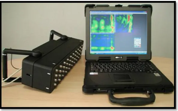
Figure 21: LMS VB8 data acquisition system ... 47

Figure 22: USQ supplied stands used to support beam during experiments ... 48

Figure 23: Graphical representation of the EMD process (Hassan 2005) ... 51

Figure 24: Experimental Process and System Overview Diagram ... 54

Figure 25: Cross-sectional area ... 55

Figure 26: USQ supplied marked composite beam with accelerometer fixed in place ... 57

Figure 27: Raw imported data and calibration ... 58

Figure 28: Truncated acceleration data ... 59

Figure 29: Single and double pass filter examples ... 59

Figure 30: Velocity data ... 60

Figure 31: Deflection data ... 60

Figure 32: IMF stage 1, node 1 ... 61

Figure 41: Instant. frequency and amplitude stage 1, node 1 ... 67

(9)

List of tables

Table 1: Damage introduction scale ... 56

List of equations

Equation 1: Trapezoidal rule (Mathews and Fink 2004) ... 32

Equation 2: Midpoint method of integration (Mathews and Fink 2004) ... 32

Equation 3: Simpson’s method of integration (Mathews and Fink 2004) ... 33

Equation 4: Short-time Fourier transformation (Barnhart 2011) ... 35

Equation 5: Refresh of Simpson’s method of integration (Mathews and Fink 2004) ... 50

Equation 6: Expression of the sifting process (Huang, Shen et al. 1998) ... 51

Equation 7: Hilbert transformation (Huang, Shen et al. 1998) ... 52

Equation 8: Phase angle (Donnelly 2006) ... 52

Equation 9: Instantaneous frequency (Donnelly 2006) ... 52

(10)

Nomenclature

Abbreviations

HHT Hilbert-Huang Transformation

FFT Fast Fourier Transformation

EMD Empirical Mode Decomposition

IMF Intrinsic Mode Function

STFT Short-Time Fourier Transformation

FRF Frequency response function

FBG Fibre-optic Bragg Grating Sensor

LDV Laser Doppler Vibrometer

AC Alternating current

DC Direct current

PLM Product lifecycle management

SHS Square hollow section

Mathematical symbols

b Location of second data point with regards to the x axis

a Location of the first data point with regards to the x axis

f(x) Function with regards to variable x



Angular frequency (rad/s)

t Global time (s)



Local time (s)

h Extraction step toward an IMF

X(t) Signal X with respect to time

m Maxima and Minima envelope mean

H[h(t)] Hilbert transformation

PV Cauchy principle



Phase angle

f Frequency

a

Amplitude

A

(11)

Chapter 1| Introduction

Monitoring structural health is of increasing interest and significance in the world of engineering as bigger and more complex projects go ahead in a time of great climactic uncertainty and with a vast and ageing established infrastructure. The need for cheap and accurate methods of monitoring and identifying structural damage is of increasing importance. Many of the current methods of damage detection are too slow, localised, costly and inaccurate to be practically applied to new complex materials and the pressure of the demand of the current infrastructure. Therefore the intention of the researcher is to assist in the promising expanse of the body of knowledge relating to the use of dynamic (vibrational) response in monitoring structural health. Specifically for monitoring the structural health of composite structures with and without damage.

There has been considerable development in the techniques used for dynamic response analysis and these techniques show great promise as a solution to the engineering problems ahead. Dynamic methods have a number of advantages over conventional methods as they are typically destructive, non-localised, and present the possibility of integrated real time application in the absence of an experienced technician. These methods also have the advantage of being capable of testing for a broad range of defects even below the surface of the material. These factors present the opportunity, given the necessary research, to develop cheaper and more effective means to monitor the safety of the structures we create. There are an increasing number of dynamic response analysis methods which will be briefly described in the literature review and compared to some traditional damage detection methods.

Composite materials were selected as the subject as they are becoming increasingly common in modern engineering applications due to their economic and mechanical advantages. However as these materials have such a brief phase between operation and catastrophic failure, careful analysis with practical methods are of great importance for maintaining acceptable levels of safety. Despite the promising theory and results produced in lab conditions, these techniques show limited practicality in real world applications due to the introduction of noise and the added requirements of apparatus.

(12)

1.1 Background

Structural health testing is highly significant in engineering applications. As the complexity of structures and materials we used increases, so too does the need for more complex and effective monitoring methods. Parallel to these increases in complexity is an aging existing infrastructure (Doebling, Farrar et al. 1998) and high uncertainty with regards to changing climatic conditions. These factors indicate the urgent requirement for innovative and efficient methods for testing structural health.

Non-dynamic testing methods can be highly localised, slow, and costly and can require specialist operators leading to the pressure for innovation in this area. During the last few decades there has been a growing interest in the use of vibration for structural health tests and there have been a number of developments. It works by applying vibration to the structure and monitoring the response using sensory apparatus. The sensory apparatus monitors some kind of physical behaviour containing some kind of modal response. This response can be processed to find the natural frequency, modal shape, damping ratio, or frequency response function to name a few. These results can then be compared to some kind of undamaged index derived from historical measurements or FEA projections. As mentioned earlier, these methods show promise in lab conditions and theory, however, it is suggested by Doebling. et al. (1998) that the reason for such slow development in establishing a clear dynamic response testing method capable of industry practice is because of the several confounding factors involved in the application of vibration based methods of damage identification. These factors will be discussed in more detail in the literature review.

Due to availability accelerometers were used as the sensory apparatus which yielded acceleration data from various nodes spaced along the test subject. This was integrated using the Simpson’s method of

integration to double integrate the data giving the deflection signal. An impact hammer was used for excitation and was chosen as the weight of a solenoid would introduce a high degree of error into the data. The deflection data could then be transformed using the HHT giving instantaneous frequency information used to produce a beam stiffness matrix (Huang and Shen 2005). By introducing progressive stages of damage these compiled matrices were compared using a finite difference algorithm (Maia, Silva et al. 2003). These experimental results could then be assessed for feasibility for damage detection. Undamaged experimental results were validated using FEA results acquired using Abaqus (Simulia 2015).

(13)

and frequency can then be derived from this expression allowing for an AM/FM time modulated signal representation. The EMD was developed by Norden E. Huang and published in his paper entailed ‘The

empirical mode decomposition and the Hilbert spectrum for nonlinear and non-stationary time series analysis’ in 1998 (Huang, Shen et al. 1998). The EMD decomposes a signal into Intrinsic Mode Functions (IMFs). These IMFs are separate summative physical representations of the original signal and are complete and almost orthogonal to the original signal. These can be processed and reassembled by the Hilbert spectral analysis. This paper also discusses key aspects such as signal processing techniques and briefly touches on composite materials.

The discussed methods were chosen after extensive review of the existing literature which is included in the paper which can be referred to for the convenience of the reader.

1.2 Research Objectives

It was hypothesised that the use of the chosen methods would empirically justify the use of such methods in dynamic testing procedures and display the practicality of industry application. There are a number of kinds of degradation experienced by materials and the structures they form which typically require unique and specific testing procedures. These forms of degradation can occur due to wear from use, seismic activity, erosive atmospheric conditions and varying intensities of weather interaction to name a few. These events cause the lifespan of the material or structure to deviate from the expected lifespan. With the added uncertainty of the application of new innovative materials, it is important to monitor their structural integrity to establish revisions of forecasted lifespans. This is relevant to the economic management and functional capacity of the structure, and also to ensure the safety of those whom of which use the structure. For these reasons, research relating to innovative methods of structural health monitoring have become an area of growing interest in both industrial and academic communities. Innovation has resulted from such interest, however, some of the most promising techniques derived from theory and performed in lab experiments, such as dynamic response techniques, does not prove as effective when applied to real world scenarios.

(14)

The intention of the researcher was to achieve some small contribution in the way of developing such an approach to dynamic testing. Because of the short duration of this research project, a final aim of this research tasks is to produce some useful suggestions for future research that can be conducted to achieve the primary objective of the practical and widely applicable use of dynamic response testing.

The process undertaken to complete the research objectives is outlined in the following:

 Extensive review of existing literature conducted relating to methods of structural health testing, dynamic methods of structural health testing, composite material types, properties and behaviour, methods of integration, signal transformation methods, data acquisition systems and related apparatus, methods of damage indexing, and techniques for signal processing

 Formulation of investigation and methods pertinent to achieving the initial research objectives both empirically and within the expected time limitations

 Data acquisition of dynamic response of chosen composite structure when subjected to forced resonance

 Numerically solve experimental data to draw comparison and establish the effectiveness of chosen methods

 Evaluate and discuss the results and practicality of the chosen methods for identifying damage severity and location for industrial applications in a cheap, timely and accurate manner

 Reflect and discuss the pertinent findings of the research including anomalies, successfully achieved objectives and suggestions for further research

1.3 Project overview

This research project took place over the course of a year during 2015, ending on the 29th_{of October,} 2015. During this time the following report was constructed. For the convenience of the reader, the researcher has included this section giving a brief outline of the report including relevant information, method of experimentation, results of experimental investigation, and conclusive remarks in reflection of the process.

1.3.1 Chapter 1| Introduction

(15)

1.3.2 Chapter 2| Literature

Chapter 2 consists of a review of all the research found pertinent to this project scope and its objectives. Other methods of structural health testing, dynamic methods of structural health testing, composite material properties and behaviour, sensor selection, methods of integration, signal processing methods, data acquisition systems, and other hardware and software selections relevant to this dissertation were extensively discussed and referenced. At the end of each topic, the viability of each topic is discussed with some preliminary remarks regarding what topic seems most applicable to the research objectives. The method chosen from such topic discussions is outlined clearly in Chapter 3.

1.3.3 Chapter 3| Project Specifics

The completion of this project involved the broad application of apparatus and methods of analysis. As such, it was deemed appropriate by the researcher to include a section dedicated to outlining the apparatus chosen and it’s relation to the system of experiments or analysis entailed. Chapter 3 includes a description of all the pertinent apparatus and software used in the project, including a description of the material that was used and the system of dynamic response testing applied. It also gives descriptions of the arithmetic used and how this arithmetic was logically translated into code usable by Matlab’s numerical analysis and processing.

1.3.4 Chapter 4| Experimental process methodology

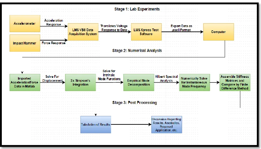
Chapter 4 outlines the procedure taken in completing the experiments involved, the data acquisition systems used, and numerical methods chosen. It has a full detailed explanation of steps and precautions taken to ensure correct scientific methods and has reference to related pictures and diagrams found in the appendix. For the preliminary report the safety procedures, inductions and timeline for important tasks are also included in this section. It also includes the resource requirements for the project. An important inclusion to the methodology section is a project system flowchart. This flowchart gives a clear and accurate description of the stages involved in the project, the systematic approach taken to completing them by the researcher, and the way in which each part of the project was related to each other with regards to analysis. This system flowchart can be found with description in Section 4.1 of Chapter 4.

1.3.5 Chapter 5| Discussion of Experimental Results

(16)

examples of the deformation achieved once the data had undergone the full double integration with all necessary applied filters. The interaction of the empirical mode decomposition was tabulated showing the results intrinsic mode functions. The instantaneous frequency of each node was then acquired by the Hilbert spectral analysis which were then assembled into a global stiffness matrix. The stiffness matrices are labelled corresponding to each particular stage of damage to which they are associated. Finally the results of the finite difference algorithm are shown and plotted. At the end of the chapter is an extensive comparison between the fast Fourier transformation results and the results of the Hilbert-Huang transformation. This comparison is presented in such a way that the physical characteristics of the response and the beam can be easily understood with brief discussions on the differences. These difference will be discussed in greater detail in Chapter 7. Each stage is briefly discussed with reference to its detailed description found in Chapter 4.

1.3.8 Chapter 6| Conclusion

(17)

Chapter 2| Literature

Before experimental investigation could begin, it was important to clarify the existing literature to gain sound knowledge regarding the concepts and to ensure that the research completed was novel and unique. A review of the literature was therefore necessary and included number of different methods for structural health monitoring and the advantages and disadvantages with relation to vibration signature methods. An explanation of the different viable methods for dynamic response testing for structural health and their respective advantages and disadvantages with relation to the method chosen in this paper is included. A review of existing software and hardware including sensory mechanisms, methods of integration and signal processing, and a method for indexing the severity of damage with relation to pristine conditions is discussed. Finally the available signal processing techniques such as filtering and transformations are discussed. The literature formed the basis for this research and in turn guided the researcher to the decision of the project aims and scope. Dynamic response methods shows limited success in industrial applications but showed potential for use without skilled operators at low cost and time required.

2.1 Traditional structural health monitoring methods

There are a number of traditional testing methods that have been used frequently in the past with moderate success regarding composites. Some of these methods include X-ray tomography, Ultrasonic tomography, dye penetration visual inspection, and coin tap testing. The literature relating to these methods, their advantages and disadvantages, and why they were not pertinent to the research is explained in this section.

2.1.1 X-ray Tomography

X-ray tomography damage detection is a non-destructive test method in which an entire structure can be screened and inspected for damage (Kinney and Nichols 1992). It involves the use of X-ray two or three dimensional imaging of an object which can then be developed by computer tomography (Kinney and Nichols 1992). However a limiting factor of the size of an object that can be practically examined by the X-ray tomography method is that the spatial resolution be kept small with respect to the microstructural properties of the material being examined. X-ray tomography has limited capabilities with regards to image micro structures such as fibres in fibre composites (Kinney and Nichols 1992).

(18)

2.1.2 Ultrasonic Tomography

[image:18.595.149.446.284.469.2]

Ultrasonic tomography is a local damage detection technique in which an ultrasonic signal is introduced to a structure. The signal is then monitored for deviations from the reference signal of an undamaged structure (Tsuda 2006). This technique uses similar principles to dynamic response techniques however the much higher frequency of ultrasonic signals (approx. 20-40 kHz according to HyperPhysics from Georgia State University) makes it only applicable for localised observation as the signal loses energy over a short distance. Once the ultrasonic signal from the object being tested is compared to the signal expected from an undamaged specimen, inconsistencies will display the nature of the damage. This technique is highly effective if prior knowledge of the location of damage is known. However this technique is not applicable for monitoring structural health of large civil structures and for the objective of this research.

Figure 1: Low-frequency ultrasonic tomograph for concrete testing (BISHKO, SAMOKRUTOV et al. 2010)

This technique has since been improved upon by (Dutta 2010). It was proposed that by the use of LAMB waves and modal data, or ultrasonic guided wave based techniques. This method was proposed to be a non-baseline technique capable of determining damage without comparison to an undamaged specimen. The data is gathered using piezoelectric wafer transducers and laser vibrometers. Vibrometers unfortunately are not applicable for the objectives of this project as it is restricted to monitoring the surface behaviour of an object. The analysis of the LAMB wave propagation is also deemed inappropriate for the objectives of this project as that testing equipment is quite costly and this method requires an experienced operator to determine the existence of damage.

2.1.3 Visual dye penetration inspection

(19)

crack. The surface dye can then be removed leave the dye that has entered the crack to stand out (Larson 2002).

Figure 2: Example of the application of visual die inspect of weld joints (Larson 2002)

Unfortunately the dye penetration method can only be used to identify surface cracks therefore is inappropriate for a range of situations. It is also highly dependent on the types of chemicals and the operators attention to detail (Larson 2002).

2.1.4 Coin tap testing

The coin-tap test is one of the oldest methods of non-destructive testing and is commonly used for testing laminated structures (Kim 2008). This method requires and operator to tap each point of a structure with a coin or hammer listening for changes in sound radiated from the structure (Kim 2008). The characteristics of the impact are highly dependent on the impedance of the structure and on the hammer or coin used (Kim 2008). The effectiveness however is highly dependent on the skill of the operator. The method is low cost due to no complicated or expensive testing equipment however it can be wrought with human inaccuracy and is limited by the thickness of the test object that can be observed. As the scope of this project is with regards to testing civil composite structures of thickness greater than a laminate this method is not relevant and will not be considered.

2.1.5 Viability of methods discussed

All the non-dynamic structural health monitoring methods discussed in this section have proven insufficient for the objectives of this project. Restrictions such as localised testing, high costs, the requirement for specialised operators, and the inability to detect at a resolution for microstructural damages have ruled out all methods discussed.

2.2 Existing dynamic structural health monitoring methods

(20)

methods. Dynamic response methods can be used to determine the existence, location and severity of the damage with varying degrees of success in each. It should be noted that the sensor system, the method of integration and the method of signal processing make quite a difference in the effectiveness of each method and are discussed in greater detail in sections 2.4, 2.5 and 2.6 respectively of the literature review.

It may seem strange that such inconclusive methods for dynamic response testing have been produced for industry application but as discussed by Doebling et al. (1998), there are a confounding number of factors making dynamic methods of damage identification difficult to apply in the practical conditions experienced in most real engineering situations. Standard modal properties represent the compression of a large spectrum of data. Modal properties are typically estimated experimentally from measured response time histories. These histories may have over one thousand data points each and if measurements are made at 100 points, there are now 100,000 pieces of data to be considered. As more innovative processing techniques are developed the method becomes more applicable to industrial applications and is now used for various industry applications in civil, mechanical and aerospace engineering.

Dynamic methods are used to analyse changes with regards to fundamental modal parameters such as the changes in natural frequency, modal strain energy, residual stress or force indicators, frequency response functions, neural networks, damping ratios and/or mode shapes (Bisht 2005). Within each of these fundamental modal parameters, various methods of acquiring the data and analysing it have been created with varying degrees of accuracy and success. Only the most common and effective methods are discussed in this section. With some less effective methods briefly mentioned in a final section.

2.2.1 Changes in natural frequency

Over the lifespan of a structure it will experience degradation in which its material properties will change accordingly. One of these material properties is the natural frequency of the object. Dynamic response testing with regards to changes in natural frequency is the practice of comparing the natural frequency of the object of interest with the expected or known natural frequency of the object in undamaged conditions (Chen, Spyrakos et al. 1995).

(21)

data. The power spectral density and magnitude of the frequency domain could be obtained by using the fast Fourier transformation. The data was then subject to linear regression to remove any noise and eradicate any baseline shift. This method concluded that an increase in damage typically decreased the expected frequency response. The location of the damage could be identified by noticing between which accelerometers showed varied frequency responses.

The accuracy of this method has been suggested that a 5% natural frequency change is the approximate requirement to be considered damage with a high reliability (Salawu 1997). However it is also mentioned that frequency changes can occur due to changes in ambient conditions. Salawu (1997) supplied notes that there have been occasions in which a 5% frequency shift has been tested conclusively when testing steel and concrete bridges in a single day.

2.2.2 Changes in modal strain energy

When a structure is subject to vibration there is strain as displacement occurs between modal nodes. Mode shapes can be recognised as the oscillating crests and troughs that form between the modal nodes. As this occurs the material experiences an increasing amount of strain on the outer minimum and maximums of the structure. Shi et al. (1998, 2000) presented a technique to identify the existence of damage by use of the mode shapes and elemental stiffness matrix. This technique requires no prior knowledge of the undamaged dynamic behaviour of the element which stands as a substantial advantage for this method. By monitoring the changes in the stiffness matrix between modal elements the location and severity of damage can be indicated. The limiting factor of this method is that the nodes of the structure being tested could introduce error in the response. The method requires a prevalent understanding of the modal nodes that is dependent on a number of factors. By analysing in a sub optimal location readings could give skewed data (Shi, Law et al. 1998, Shi, Law et al. 2000).

2.2.3 Residual force/stress indicators

Residual force indication utilises modal force vectors derived from a residual flexibility matrix to identify the existence of damage in structures (Ricles and Kosmatka 1992). The residual flexibility matrix can be found by measuring the contribution of the materials flexibility matrix from modes outside the measured bandwidth (Doebling, Farrar et al. 1998). This method was developed to solve iteratively for optimisation problems using the Gauss-Newton method (Chen and Nagarajaiah 2007).

(22)

2.2.4 Neural Networks

Neural networks, while in a primitive form, is a type of artificial intelligence. Digital computers operate in an entirely different manner than a natural brain however the function of a neural network is to create a systemic network connecting functions depending on events such as monitoring results data from sensory equipment and processing the data into a numerous amount of frequency response functions (Wu, Ghaboussi et al. 1992). This technique has been used by Castellini & Revel et al. (2000) involved the application of Laser Doppler Vibrometry as a sensory apparatus and the data was processed by the trained neural network. The sensory apparatus retrieved the vibration velocity spectra from a series of points on a test panel which could then be derived into displacement data by the neural network (Castellini and Revel 2000). The truly incredible thing about neural networks is the way in which it is trained. It becomes more functional by acquiring knowledge from its environment by use of learning algorithm which is capable of modifying synaptic pathways or synaptic weights (Haykin 2004).

This technique is highly promising and can be used to combine the advantages of multiple techniques to compile a more accurate hypothesis of the true nature and location of damage in a structure. However as such a technique requires much more time than available for the completion of this project this method was not chosen. It is however a desirable project in itself for further research and due to time constraints lies outside the scope of this project.

2.2.5 Changes in damping ratios

Damping is typically an irreversible process of converting mechanical vibration into heat as a result of motion(Rao 2005). It occurs due to friction factors internal or external of the material. Use of the change in damping ratio to analyse structural damage has been done by Abeykoon & Kawarai. et al. (2015) by decomposing modal damping ratios into mode-independent damping parameters of energy-dissipating sources in bridges (ABEYKOON, KAWARAI et al. 2015). Change in damping parameters can then be used to detect damaged structural components.

2.2.6 Changes in mode shapes

(23)

This method has been effective at identifying the location of damage subjected to a structure however is less effective at indicating the severity of the damage (Doebling, Farrar et al. 1998). This method has seen continual improvement. Such improvements include experiments by Kim & Stubbs (2002) in which have worked continually to improve the methods accuracy by removing erratic assumptions and limits existing in the related algorithms (Kim and Stubbs 2002).

This method was not considered viable for the project however as it has been noted by Maia & Silva et al. (2003) to be time consuming and fraught with numerous errors related to the curve fitting algorithms.

2.2.7 Changes in frequency response functions

There are several different definitions of frequency response functions. Frequency response functions (FRF) is a method similar to previously discussed methods in that it uses some combination of changes in natural frequency, damping and modal interaction (Lee and Shin 2002). however it involves the analysis of the structure at a range of different frequencies (Maia, Silva et al. 2003). Experiments completed by Maia & Silva et al. (2003) and Sampaio (1999) indicate that this method is much more accurate than the mode shape method. The FRF method works by collecting mode shape data at numerous standard frequencies for either a damaged and undamaged structure or section in order to detect local differences in the flexibility of the damaged and undamaged response. The four different types of analysis discussed in the mode shapes method being mode shape, mode shape curvature, mode shape curvature squared, and mode shape slope are the behaviours considered for analysis in this method also (Sampaio, Maia et al. 1999, Maia, Silva et al. 2003).

The FRF method works by analysis of several sets of deflection and oscillating force data. This data can then be used to construct a flexibility matrix. This matrix can then be analysed by use of a damage index algorithm. This method typically requires a lot of nodes as accuracy is lost with large nodal spacing (Fu and He 2001). FRF methods typically require smaller frequency ranges as higher frequency range bring about the inclusion of a large number of modal frequencies. Increased modal frequencies also require more intensive calculations (Sampaio, Maia et al. 1999, Fu and He 2001). This is because the FRF relies on higher stiffness changes which becomes less significant when compared to the amplitude difference of the frequency shift due to resonance (Sampaio, Maia et al. 1999, Fu and He 2001). For the FRF to be effectively applied, frequencies close to but before the first resonance or anti-resonance frequency is desirable.

(24)

frequency response of the model” the location and extent of the damage can be identified to a high degree of accuracy (Schulz, Pai et al. 1996). This optimisation comes at a large increase in required computational capability.

2.2.8 Change in mechanical impedance

Impedance based structural health monitoring have been developed using the electromechanical coupling property of piezoelectric materials (Sun, Rogers et al. 1995). This is a non-destructive testing method that utilises the electromechanical coupling property of piezoelectric materials. Because structural mechanical impedance measurements are difficult to obtain, changes in electromechanical impedance reactions of piezoelectric sensory equipment is more effective. This sensory system is used to monitor changes in structural stiffness, damping and mass (Park and Inman 2005).

2.2.9 Viability of methods discussed and method chosen

The frequency response functions and changes mode shapes are both desirable methods for the purpose of this project according to the literature that has been reviewed. However, a decision between the two is highly dependent on the transform method chosen in further sections. The final decision on viable dynamic response method was to monitor the variations instantaneous frequency response functions. Changes in mode shapes was considered as a secondary tasks however was highly dependent on time as the project was conducted over only one year.

2.3 Composite materials

A composite material is required for vibration based structural health testing and the literature relating to composites is discussed in this section including a brief explanation of what constitutes a composite. There is also an explanation with regards to the viability of each composite type which said discussion indicates briefly the direction of thought involved in choosing the material used to collect experimental data.

(25)

This Section discusses some of the more common or advanced types of composites, their advantages and disadvantages and some practical applications for which they are used. It also outlines the feasibility of these materials with regards to the experimental investigation outlined in this report. While alloys can be considered a composite material, they lay outside the scope of this project as the purpose is to investigate the ability of structural health monitoring of a non-monolithic composite materials. Fibre composites are the focus and different kinds are discussed in this section as they present a difficult task to structural health monitoring. They do not consist of uniform material properties and are typically mechanically orthotropic. Other kinds of composites include Particle reinforced materials, nanomaterial reinforced materials and structural laminates or sandwich panel arrangements (William D. Callister and Rethwisch 2014). There are some less common composite materials that are not discussed in this section as they are not commonly used and these include boron, silicon, carbide and aluminium oxide and nanomaterial composites.

2.3.1 Glass fibre-reinforced polymers

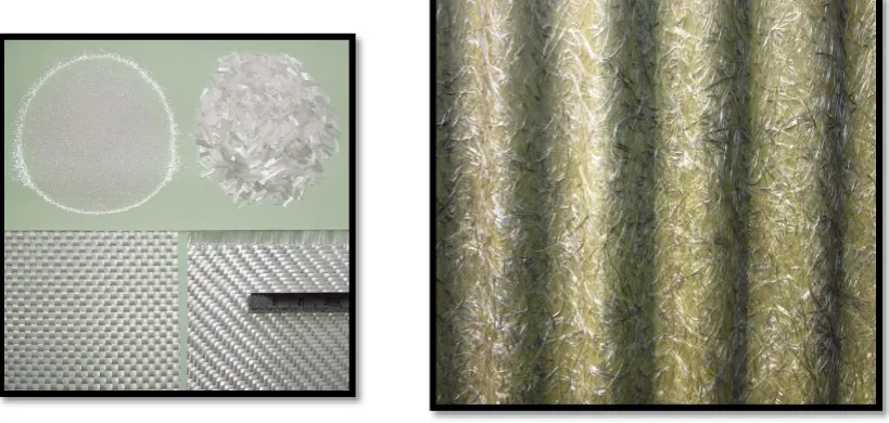
Fibreglass is one of the most common and familiar composites (William D. Callister and Rethwisch 2014). It was one of the first clearly classified composites as the field was being established in the mid-20th_{century as it became highly applicable to the construction of boats and soon storage tanks, houses} and plastic pipes to name a few of its applications. It consists of glass fibres, either in continuous or discontinuous arrangement, contained within a polymer matrix. This composite is the most vastly produced. Fibres are typically between 3 and 20 micrometres in diameter and are classified by either long or short length fibres (William D. Callister and Rethwisch 2014).

Figure 3: Corrugated resign reinforced glass fibre composite (Kittinger-Sereinig 2015)

[image:25.595.76.486.491.686.2]

Figure 4: Glass fibres (Jean-Pierre 2009)

This is most popular or the fibre composites due to the following advantages:

 Easily manufactured by drawing into high strength fibres from molten state

(26)

 Applicable to multiple shapes and component functions

 Wide variety of manufacturing techniques

 Glass fibres are relatively strong and when embedded in a polymer matrix yields a very high specific strength

 Various polymer types can yield high chemical resistance making it ideal for corrosive environments

 Resistance to heat, fire and maintains dimensional stability in high temperature environments

 Electrically inert

There are challenges to this material however as interaction with another hard material can introduce surface flaws. Surface characteristics of glass fibre composites are very important and small defects can change the tensile properties by a great deal (William D. Callister and Rethwisch 2014). Some disadvantages of this material include:

 Specific applications to ensure no interaction at surface with other hard materials

 Low stiffness and rigidity

 Limited to applications below approximately 200 degrees Celsius depending on the polymer matrix used but can be extended as high as 350 degrees Celsius if cast in high purity infused silica

 There are possible health risks in handling if necessary safety precautions are not considered and met in practice

 Low Fatigue performance limits compared to other fibre composites

2.3.2 Carbon fibre-reinforced polymers

Carbon fibre is typically used in high performance material used in advanced polymer matrix composites. Some of the advantages of carbon fibre-reinforced polymers include:

 Carbon fibres have high specific moduli (elastic modulus per mass density) and high specific strength

 They retain high elasticity and strength at elevated temperatures however at high temperatures the carbon can becoming reactive with oxygen

 At room temperature carbon is unaffected by moisture or a wide variety of acids, solvents and bases

 Diverse range of desirable material properties therefore is applicable for a number of engineering applications

 Carbon fibre and composite manufacturing methods have been developed that are reasonably inexpensive and cost effective

(27)

Figure 5: Carbon fibre matting (Hadhuey 2005)

While the price of manufacture has decreased considerably with modern techniques it is still high in comparison to other fibre composites which is one of the first disadvantages. This makes it for specific and advanced applications. The list of disadvantages experienced by this fibre composite are as follows:

 High cost of manufacture compared to other fibre composites

 Carbon fibres can have resign compatibility issues therefore epoxy resigns are typically used which causes a further increased cost in finished products

 Carbon fibres is not as easily manufactured and the materials are not as readily available as other fibre materials

2.3.3 Aramid fibre-reinforced polymers

[image:27.595.159.435.73.284.2]

Aramid fibres are high strength and high modulus materials that are commonly used in aerospace and military applications. There are a number of different types however the most common types are made from Kevlar or Nomex. These fibre composite materials have superior strength to weight ratios than metals.

Figure 6: Aramid fibre matting (Jean-Pierre and Jaybear 2012)

(28)

 High toughness, impact resistance, and resistance to creep and fatigue fracture

 High tensile strength

 Chemically resistant except by strong base or acid chemicals

 Even though they are thermoplastics they retain their mechanical properties from around -200 to 200 degrees Celsius

The disadvantages of aramid fibre-reinforced polymers are as follows:

 Poor compression strength due to micro buckling and poor performance when subject to traverse loading as bonding between fibres is typically weak

 Sensitive to ultraviolet radiation

 Absorbs moisture

2.3.4 Viability of composites discussed

Glass fibre-reinforced polymers were decided upon for the experimental analysis in this project for two reasons. Firstly because they are the most widely used in industrial applications, therefore increasing the body of knowledge surrounding this particular material will be widely beneficial to the engineering community. The second reason being that this material is cheap and readily available at the university as it is a common material made for other research here at USQ.

Glass fibre pultruded square hollow section beams are used as there are readily cast members available. Pultrusion is the process of pulling glass fibres of a spool through a polymer injection process. Long strands of glass fibre run right through the polymer giving high tensile strength in close to orthotropic uniformity.

2.4 Sensors for experimental data acquisition

Various data acquisition sensors are suitable for the analysis of dynamic response in structures. This section discusses the function, advantages and disadvantages of various sensors and the reason for the chosen sensor. As there are a number of dynamic response methods requiring different forms of data sensors are typically more suitable for certain methods therefore the type of sensor is primarily related to the chosen dynamic testing method chosen however as discussed in the following sections there are a number of suitable sensors for testing this projects chosen dynamic response method.

(29)

2.5.1 Accelerometers

Accelerometers are micro electromechanical systems used to convert acceleration into electrical voltage signals. Accelerometers require calibration so that the voltage response responds to the correct acceleration. The calibration is typically the largest source for error however accelerometers are proven to provide highly accurate data (Kuehnel and Sherman 1994). Accelerometers involve micro electromechanical structures made from piezoelectric materials such as quartz.

Figure 7: Accelerometer components diagram (Raki 2013)

Accelerometers are cheap components that are readily available at the university. Using this kind of sensory component would retrieve data in the form of acceleration therefore an effective integration method would be necessary to convert this data into displacement if this were to be chosen for experimental data acquisition.

2.5.2 Fibre-optic Bragg Grating Sensors

(30)

Figure 8: Fibre-optic Bragg grating sensor optical function diagram (Rusaw 2010)

Optical fibre sensors are immune to electromagnetic interference, light weight, small, have a high sensitivity, a large bandwidth and are easily implemented. While they have high sensitivity, their sensitivity to the specific application of sensing low amplitude vibrations is only of a moderate standard (Lee 2003). Spectral decoding methods cannot be utilised to detect high frequency signals due to the inherent low speed of the optical fibre sensing method (Wild and Hinckley 2010).

2.5.3 Laser Doppler Vibrometers

Laser Doppler Vibrometers (LDV) is a remote, non-destructive and high spatial recognition method of vibration based structural health monitoring. LDV has a high frequency bandwidth, up to 20 MHz, a velocity range of ±30 m/s, resolution of about 8 nm and displacements of 0.5 μm/s (Castellini, Martarelli et al. 2006). LDV’s monitor instantaneous velocity data of objects subjected to oscillating loads. The LDV produces a laser directed at the surface of interest. Any vibratory behaviour will cause a Doppler shift in the reflected laser beam frequency (Castellini, Martarelli et al. 2006). The beams instantaneous frequency shifts can be translated to yield the instantaneous changes in velocity experienced at the surface.

Figure 9: LDV system diagram (Wang, Li et al. 2011)

(31)

2.5.5 Viability of Sensory Systems Discussed

Both FBG sensors and accelerometers are available for use in the present experimental facilities. However, as previously mentioned LDV systems are of high cost and unavailable for use in these experiments. A comparison made by reference to the literature suggests for detecting vibration in a solid object that the accelerometer will yield more accurate results. Therefore it was decided that the accelerometer would be the correct sensory apparatus for use in this projects experiments.

2.5 Methods of Integration

Using accelerometers to collect the dynamic response data, as suggested above, will lead to the acquired dynamic response consisting of acceleration data. It is required that acceleration be integrated twice in order to acquire the displacement data. Only then can the data be applied to a signal transformation and graphically represented for clear analysis. There are three suitable methods of integration that will be discussed and considered in this section (Heaton 2011).

Other important considerations are the sources of error in these methods and some of the proposed optimisation techniques that have surfaced in scientific literature. Noise is a major contributor to the error introduced to these techniques (Stiros 2008). Some unavoidable error can of course be contributed to the characteristic limitations of sensory apparatus, however, the majority of error during dynamic response tests will be attributed to the overwhelming effects of noise.

2.5.1 Trapezoidal Rule

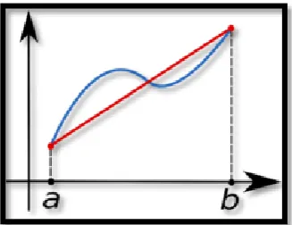
[image:31.595.215.379.594.720.2]

The trapezoidal rule, or trapezium rule, is considered the simplest numerical methods for integrating. It works by breaking the function up by each of its data points and calculating each section based on strips where the data points are connected in a linear fashion (James 2008). The area of a series of trapezoids can be easily found therefore calculating the area under the curve is an easy tasks for numerical analysis. It should also be noted that the more dense the data points, the greater the accuracy of this method (James 2008). The area under a curve can be approximated by the trapezoidal rule which is expressed as the following:

(32)

Equation 1: Trapezoidal rule (Mathews and Fink 2004)

( )

(

)

2

b a

f a

f b

f x dx

  

b a















Where:

b

is the location of the second data point with regards to the ‘x axis’

a

is the location of the first data point with regards to the ‘x axis’

This formula can be applied to a function with ‘n’ number of data points ‘n-1’ times yielding the approximate area under the curve of a data set or signal. As the figure suggests, having more frequent data sets spaced more closely together yields a more accurate integration.

2.5.2 Midpoint Rule

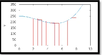
[image:32.595.211.385.367.461.2]

The midpoint rule, or rectangle rule, is an integration technique used to integrate data in which two points are used as boundaries and an equation to find a suitable midpoint between the data points can be found (Burden and Faires 2011). This midpoint is then included as a data point and a typical integration method such as the Trapezoidal is used to integrate (Burden and Faires 2011).

Figure 11: Midpoint rule geometry example (Alexandrov 2007)

This method can be considered an extension of another method to possibly increase the accuracy of the base method. This method was improved by Fink and Mathews et al. (2004) in which it was demonstrated how an error factor can be considered depending on the method and midpoint function used (Mathews and Fink 2004). The midpoint rule can be expressed as the following:

Equation 2: Midpoint method of integration (Mathews and Fink 2004)

1 0

( )

N b n a n

f x dx

h

f x











(

) /

h



b



a

N

n

x  a nh

Where:

b

a

N

is the number of equally divided subintervals

h

is the length of subintervals

n

(33)

2.5.3 Simpson’s Rule

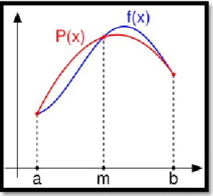
[image:33.595.220.375.171.313.2]

This numerical method of integration is an approximation of definite integrals using quadratic and Lagrange polynomial interpolation between data points (James 2008). This method is said to be significantly superior in comparison to the midpoint and trapezoidal rule in almost all situations by a number of sources (Mathews and Fink 2004, James 2008, Burden and Faires 2011).

Figure 12: Graphical example of the Simpson’s integration method (Alexandrov 2005)

One of the main advantages that the Simpson’s rule has over other more conventional methods of integration is that it can be used to more accurately estimate the curve as the shape between data points can be estimated more accurately. Its advantage over the other methods becomes more apparent as the distance between data points increases. The equation used in this method corresponding to the figure above is shown below:

Equation 3: Simpson’s method of integration (Mathews and Fink 2004)

( )

4

( )

6

2

b

a

b

a

b

f x dx



 



f a



f













f b















Where:

b

a

After the review of the literature numerous sources have pointed to the Simpson’s method of integration as the most accurate. This is because it is best capable of fitting the curve between data points using both quadratic and Lagrange polynomials as a method of interpolation.

2.6 Damage Indexing

(34)

sensors in multiple locations, the location in which the signal experienced an abnormal change could conclusively be determined to be near where the damage occurred (Maia, Silva et al. 2003). By identifying at exactly what location this abnormality occurred, it could be determined that the damage lie between that sensor and the sensor preceding it. This method requires closely localised sensory arrangements to be effective with current techniques making it slow and costly.

It may be possible to employ this technique in a more effective way by using it in cognition with a different transformation process. Research using the Hilbert-Huang technique of transformation has demonstrated the possibility of finding damage location based on a moving force generator, with known location related to time, with only one data acquisition node. The known force creation device, such as a car driving across a bridge monitored by one sensor location, is one such example of how this technique could be applied (Roveri and Carcaterra 2012). This works as the Hilbert-Huang transformation allows the user to analysis nonlinear and non-stationary signals. If the force creating apparatus moves the signal can still be analysed and a change can be noticed depending on at what position the apparatus is when a change of signal behaviour occurs. This method is highly dependent on the range of the sensor and with increasing distance, noise is to be expected. Over larger distances more sensors would still be required in order to establish effective dynamic response sensing.

Once the response has been translated into data by sensory apparatus, processing and indexing the location and severity of damage can be conducted. Indexing the damage severity can be done in a number of ways and is dependent on the dynamic or non-dynamical method chosen for damage detection. As only dynamic methods are to be considered in this research, they will be solely discussed.

2.7 Signal Transformation Method

Methods for signal transformation, also known as signal processing, are the possible ways of interpreting the results received by the data acquisition system. They work by converting the mechanical vibratory displacement signal into a series of fundamental signals used creating a series frequency dependant functions and possibly time-frequency dependant. These signals are more easily analysed for changes in behaviour once separated.

2.7.1 Fast Fourier Transformation

The fast Fourier transform (FFT) is a Fourier transformation with discrete boundaries which reduces

the computations needed for

N

number of points from 2

(35)

This transformation method proves problematic when the waveform deviates from sinusoidal and is for analysing stationary data. In typical structural health monitoring situations sinusoidal and stationary vibratory response may not be a practical or achievable outcome. While given that in the controlled circumstances of experiments this may be met, the purpose of this project is to optimise methods capable of practical application therefore this method was deemed inappropriate for the scope of this project.

2.7.2 Short-Time Fourier Transformation

The short-time Fourier transform (STFT) is a computationally simple method of estimating sinusoidal frequency and phase content of local sections of a signal. To compute the STFT a signal is divided into smaller sections that can then be separately analysed by use of the Fourier transform. A Fourier spectrum is then constructed out of the segments which can be plot as a function of time (Griffin and Lim 1984).

Equation 4: Short-time Fourier transformation (Barnhart 2011)

1

( , )

( ) (

)

2

i

STFT



t

f t h t



e



d

















Where:

STFT

is the short-time Fourier transformation (Hz)

h

is the window function

t

is the global time value (s)



is the local time value (s)



_{is frequency (rad/s)}

This approach is typically optimised by use of the continuous-time STFT. This requires that the function is then multiplied by a window function, which performs a similar function to that of dividing the signal into smaller sections, however it operates on a continually repetitive basis. The Fourier transform is then taken as the window function continually isolates segments of the signal. The results from such an operation can then be used to construct a two-dimensional (time and frequency) representation of the data (Allen and Rabiner 1977).

There is considerable error introduced by the window function’s refresh frequency. Many techniques using similar repetitive application methods similar to the window function all suffer from the same accumulative error (Kadambe and Boudreaux-Bartels 1992).

2.7.3 Wavelet Shape Matching

(36)

frequency and amplitude, but with particular attention paid to the application of peak detection algorithms (Du, Kibbe et al. 2006). For such algorithms to function effectively, signals are typically subject to operations known as smoothing and baseline correction. This causes the shape of the signal function to substantially change in the case of complex signal responses (Belongie, Malik et al. 2002). Most peak detection algorithms simply identify peaks and amplitude while ignoring any additional information present in the signal. Belongie et al. (2002) produced a continuous wavelet transform based peak detection algorithm that identifies peaks at different scales and amplitudes (Belongie, Malik et al. 2002). While this innovative technique greatly increased the robustness of peak detection under a variety of conditions, the error introduced by the shape matching factor still proves to be of considerable magnitude. This technique becomes more effective as the signal approaches one of the shape of one of following waveforms:

1. Sine waveform – The sine waveform is the most common of all the electrical waveforms as it is the function explaining the behaviour of alternating current (AC). This is used for AC mains which is the form that current is transferred over distances (Storr 2015).

Figure 13: Sinusoidal waveforms (Storr 2015)

2. Square-wave waveform – These waveforms are used extensively in electronics for timing and control signals. These symmetrical square waveforms are of equal duration, each representing each half of a cycle and used in nearly all digital input and output logic gates.

Figure 14: Square waveforms (Storr 2015)

(37)

[image:37.595.162.428.383.497.2]

3. Triangular waveforms – Triangular waveforms are bi-directional waveforms that oscillate between positive and negative peak values. Generally, the positive slopes and negative slopes have the same cycle time giving each triangle a 50% duty cycle. Triangle wave forms can also be used in an unsymmetrical form known as sawtooth waveforms. Saw-toothed waveform properties make them highly applicable to harmonics and is the wave form aimed to be produced in music synthesis.

Figure 15: Triangular sawtooth waveforms (Storr 2015)

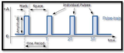
4. Triggers or pulses - The only difference between these two waveforms is that triggers can be positive or negative while pulses are only positive. Pulses and triggers are typically used to trigger something to begin such as an electromechanical system or event.

Figure 16: Pulse waveforms (Storr 2015)

This technique is highly sensitive to the amount of smoothing and baseline correction that the original signal is subject to and therefore introduces a great deal of error when analysing complex signal such as dynamic response of materials (Du, Kibbe et al. 2006). Even considering the optimisation conducted by Belongie et al. (2002) this method was deemed not accurate enough for application to the complex signal of fibre composite’s dynamic behaviour.

2.7.4 Hilbert-Huang Transformation

(38)

accuracy of the time span of the window (Donnelly 2006). One other method used to analyse a signal with regards to frequency and time, is by employing pre-defined functions to match portions of the signal. This technique proves insufficient as the complexity of the response increases. This leaves the method in question. The largest advantage of the HHT over previously discussed methods is that the

Hilbert-Huang transformation (HHT) (Huang, Shen et al. 1998) represent data in both the time and frequency domain simultaneously without a great burden on computational processing capabilities. The simplicity and robustness of the HHT are the main advantages of the technique but there are still sources of error inherent to this technique that will be discussed in detail further in this section.

After the Hilbert transform has been computed the arc tan of the real part divided by the complex part yields the phase. Unwrapping the phase causes the signal to increase monotonically. Finally the frequency is found as the derivative of the phase divided by 2pi and the amplitude is determined as the vector magnitude of the real and complex components. The arithmetic pertaining to the discussed method can vary therefore only the most pertinent equation forms have been included. These equations after selection can be found in section 3.4.

By use of the HHT, the instantaneous change in frequency, or frequency response data is used to analyse structural damage and location to a high degree of accuracy depending on the influence of noise (Roveri and Carcaterra 2012). The use of this processing technique can also remove the requirement for prior knowledge regarding dynamic response of the beam and reduces the number of data acquisition points to one assuming within reasonable distance of the damage location and that the source of the dynamic signal is non-stationary (Roveri and Carcaterra 2012). The HHT method is more accurately known as a combination of two fundamental mathematical formulations, which includes the empirical mode decomposition (EMD) and the Hilbert Spectral analysis (Huang, Shen et al. 1998). The Hilbert spectral analysis can also be broken down into sub-fundamental mathematical formulations as it performs a spectral analysis of the signal using the Hilbert Transform followed by an instantaneous frequency computation.

The empirical mode decomposition

The function of the EMD is to identify proper time scales that reveal elements representing the physical characteristics of a signal. These elements are intrinsic to the signal function which are referred to as

Intrinsic Mode Functions (IMF) (Huang, Shen et al. 1998, Zhang, Price et al. 2008). These IMFs must satisfy the two following basic conditions:

1. In the whole dataset of an IMF, the number of extrema and zero crossings must be equal or differ by at most one.

(39)

The EMD is an iteratively applied process that is continued until the above criteria are met. Suppose it is used to decompose the signal in the figure below.

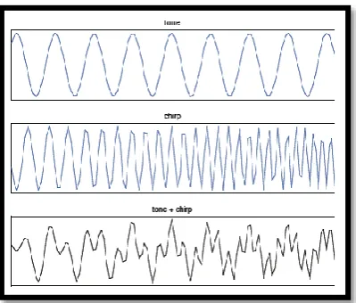
Figure 17: Original signal to be analysed (UC-San_Diego 2014)

[image:39.595.197.397.110.280.2]

The tone and the chip make for a signal more complex than a simple sin wave. This prevents analysis by means of conventional arithmetic. Using a cubic spline, the maxima and minima can be interpolated creating what is known as envelopes. The mean value between these envelopes will follow a progression between these peaks resembling a low frequency component of the signal. The positive, negative and mean interpolations are displayed in the following figures as the red, blue and purple lines respectively.

Figure 18: IMF 1, Iteration 0 and 2 displaying residue (UC-San_Diego 2014)

(40)

1. The absolute amplitude of the remaining signal is close to zero 2. The