University of Southern Queensland
Faculty of Health, Engineering and Science
Analysis of Steady State Vs Dynamic Modelling of
Groundwater Mounding in Development Areas in WA
A dissertation submitted by
Luke Rusconi
In fulfilment of the requirements of
ENG4111 and ENG4112 Research Project
towards the degree of
Bachelor of Engineering (Civil)
Page | i
Abstract
In Western Australia, a key design requirement in the land development industry is to ensure that finished lot levels have sufficient separation to groundwater levels. This is to ensure the practical and economic construction of dwellings, as well as to protect the amenity of the dwellings and provide recreational areas and gardens that are not water logged and fit for use. To achieve this there are two standard methodologies used within the industry being, the filling of lots to gain separation and/or the provision of adequate subsoil drainage to lower and control groundwater. The cost of importing fill to
Page | ii University of Southern Queensland
Faculty of Health, Engineering and Sciences
ENG4111 & ENG4112 Research Project
Limitations of Use
The Council of the University of Southern Queensland, its Faculty of Health, Engineering & Sciences, and the staff of the University of Southern Queensland, do not accept any responsibility for the truth, accuracy or completeness of material contained within or associated with this dissertation.
Persons using all or any part of this material do so at their own risk, and not at the risk of the Council of the University of Southern Queensland, its Faculty of Health, Engineering & Sciences or the staff of the University of Southern Queensland.
Page | iii
Certification
I certify that the ideas, designs and experimental work, results, analyses and conclusions set out in this dissertation are entirely my own effort, except where otherwise indicated and acknowledged.
I further certify that the work is original and has not been previously submitted for assessment in any other course or institution, except where specifically stated.
Luke Rusconi 07/10/2016
Page | iv
Acknowledgements
I would like to acknowledge the Executive General Manager of Calibre Consulting (Aust) WA, Wayne Edgeloe for his support over the last 6 years. Without the flexibility of being able to work my study time into my full time work hours this would not have been possible. I would also like to thank Wayne for his technical assistance on this research project and acknowledge that the idea of applying monthly averaged flows to steady state equations was first introduced by Wayne.
Page | v
Table of Contents
Abstract ... i
Acknowledgements ... iv
Table of Figures ... vii
List of Tables ... viii
1.0 Introduction ... 1
1.1 Aims and Objectives ... 2
2.0 Literature Review ... 3
2.1 Study Area ... 3
2.2 Location ... 3
2.3 Groundwater Characteristics ... 5
2.4 Unsaturated Flow ... 6
2.5 Saturated Flow ... 6
2.6 Hydraulic Conductivity ... 7
2.7 Specific Yield ... 8
2.8 Steady State Flow ... 8
2.9 Unsteady or Transient Flow ... 9
2.10 Swan Coastal Plain Groundwater Environment ... 9
2.11 Dwellings, Buildings, Development Issues... 9
2.11.1 An Overview of Western Australian Drainage Design Principles ... 9
2.11.2 Relevant Legislation and Guidelines in Western Australia... 12
2.11.2.1 Models ... 13
2.11.2.2 Boundary/Initial Conditions ... 13
2.11.2.3 Geotechnical and Hydrological Parameters ... 14
2.11.2.4 Separation Distances ... 15
3.0 Steady State Equations ... 17
3.1 Darcy’s Law ... 17
3.2 Dupuit Theory ... 17
3.3 Darcy’s Law Hillman and Cocks Application ... 18
3.4 Hooghoudt Equation ... 20
4.0 Dynamic Model - Unsteady state ... 22
4.1 MODFLOW GMS (Aquaveo) ... 22
5.0 Methodology ... 24
5.1 Collation of Site Specific Data ... 24
5.2 Model Development ... 25
5.2.1 Hooghoudt Equation ... 25
Page | vi
5.2.3 Darcy/Dupuit Equation ... 26
5.2.4 MODFLOW – Steady State ... 27
5.2.5 MODFLOW – Transient ... 28
6.0 Analysis ... 30
6.1 Theoretical Test Case One (90m Separation) ... 30
6.1.1 Results ... 30
6.2 Theoretical Test Case Two (90m Separation Soak wells at Rear) ... 32
6.2.1 Results ... 34
6.3 Theoretical Test Case 3 and 4 (60m, 35m Separations) ... 36
6.3.1 Results Test Case 3 ... 36
6.3.2 Results Test Case 4 ... 37
6.4 Theoretical Test Case 5 (90m Separation No Soak wells) ... 40
6.4.1 Results Theoretical Test Case 5 ... 40
6.5 Theoretical Test Case 6 (60m Separation No Soak wells) ... 42
6.5.1 Results Theoretical Test Case 6 ... 42
6.6 Theoretical Test Case 7 (35m Separation No Soak wells) ... 43
6.6.1 Results Theoretical Test Case 7 ... 43
6.7 Theoretical Test Case 8 (Capped Daily Maximum Rainfall) ... 45
6.7.1 Results Theoretical Test Case 8 ... 45
6.8 Theoretical Test Case 9 (Hillman Cocks Modifications) ... 46
6.8.1 Results Theoretical Test Case 9 ... 47
6.9 Theoretical Test Case 10 (90m Transient Soak wells at Rear, Soak wells at Front Comparison) ... 49
6.9.1 Results Theoretical Test Case 10 ... 49
6.10 Theoretical Test Case 11 (60m Transient Soak wells at ... 50
Rear, Soak wells at Front Comparison) ... 50
6.10.1 Results Theoretical Test Case 11 ... 51
6.11 Theoretical Test Case 12 (Street Drainage Model) ... 51
6.11.1 Results Theoretical Test Case 12 ... 53
6.12 Theoretical Test Case 13 (One Out of the Box!) ... 53
6.12.1 Results Theoretical Test Case 13 ... 54
7.0 Results Discussion ... 57
7.1 Steady State Vs Transient ... 57
7.2 Soak Wells at Back Vs Soak Wells at Front ... 57
7.3 Soak Wells Vs Drain Connected ... 58
7.4 Validity of the IPWEA Guidelines ... 59
7.5 Efficiencies in Design ... 59
Page | vii
8.0 Conclusion ... 62
9.0 Recommendations ... 64
10.0 References ... 65
11.0 Appendix A (Project Specification) ... 67
Table of Figures
Figure 1 – Typical soil Characteristics (Calibre Consulting (AUST) Pty Ltd) ... 4Figure 2 – Dunsborough Rainfall Intensities (Bureau of Meteorology) ... 5
Figure 3 – Groundwater definitions Source: USGS Sustainability of Ground Water Resources 1999 (Alley, MA, Reilly, TE, Franke, OL 1999 p6) ... 6
Figure 4 – Typical Particle Size Distribution for Fill Sand in the Dunsborough Region. (Calibre Consulting (Aust) Pty Ltd) ... 7
Figure 5 – Typical mounding under steady state conditions: Drainage Principles and Applications (Ritzema HP 1994) ... 8
Figure 6 – Typical Subsoil Details (Calibre Consulting (Aust) 2016) ... 10
Figure 7 – Typical Residential Onsite Drainage Systems ... 10
Figure 8 – Groundwater mounding requirement (Calibre Consulting (Aust) Pty Ltd) ... 11
Figure 9 – Correlation between phreatic surface and deemed to comply separation - Draft Specification distances for groundwater-controlled urban development (IPWEA 2016 p12) ... 16
Figure 10 – Hillman Cocks Method ... 19
Figure 13 - MODFLOW cells (U.S. Geological Survey) ... 22
Figure 14 – Steady State Flow Spreadsheet Hooghoudt Equation ... 25
Figure 15 – Steady State Flow Spreadsheet Hillman Cocks Method... 26
Figure 16 – Steady State Flow Spreadsheet Darcy/Dupuit Equation ... 27
Figure 17 – XY Grid Layout MODFLOW ... 28
Figure 18 – Theoretical Case 1 Comparison ... 30
Figure 19 – Distribution of Recharge ... 33
Figure 20 – Head distribution for soak wells located at the front of lot... 33
Figure 21 – Head distribution for soak wells located at the rear of lot ... 34
Figure 22 – Theoretical Case 2 Comparison ... 34
Figure 23 – Theoretical Case 3 – 60m Comparison ... 36
Figure 24 – Theoretical Case 4 – 35m Comparison ... 38
Figure 25 – Theoretical Case 5 – 90m Comparison (no soak well recharge) ... 41
Figure 26 – Theoretical Case 6 – 60m Comparison (no soak well recharge) ... 42
Page | viii Figure 28 – Theoretical Case 8 – Comparison 62mm event replaced by 30mm event Soak
wells at Rear ... 45
Figure 29 – Theoretical Case 8 – Comparison 62mm event replaced by 30mm event drains connected ... 46
Figure 30 – Theoretical Case 9 – Comparison Drain Connected to modified Hillman Cocks Method. ... 49
Figure 31 – Theoretical Case 10 – Comparison Soak wells at front to transient models.. 50
Figure 32 – Theoretical Case 11 – Comparison Soak wells at front to transient models.. 51
Figure 33 – Typical road profile. ... 52
Figure 34 – MODFLOW Grid layout. ... 52
Figure 35 – Street Drainage Mounding Distribution. ... 53
Figure 36 – Alternative Groundwater Control Method. ... 54
Figure 37 – Theoretical Case 13 – Comparison Alternative Subsoil Model. ... 55
Figure 38 – Theoretical Case 13 – Mounding Distribution. ... 55
List of Tables
Table 1 – Indicative saturated hydraulic conductivity values for various soil mediums (UNSW 2007) ... 8Table 2 – Summary of groundwater modelling requirements – Draft Specification distances for groundwater-controlled urban development (IPWEA 2016 p4) ... 13
Table 3 – IPWEA recommended groundwater recharge rates - Draft Specification distances for groundwater-controlled urban development (IPWEA 2016 p7) ... 14
Table 4 – Drainage infrastructure separation distance - Draft Specification distances for groundwater-controlled urban development (IPWEA 2016 p10) ... 15
Table 5 – Residential lots separation distance - Draft Specification distances for groundwater-controlled urban development (IPWEA 2016 p10) ... 15
Table 6 – Turfed Public open space separation distance based on typical soil types - Draft Specification distances for groundwater-controlled urban development (IPWEA 2016 p11) ... 16
Table 7 – Standard IPWEA Requirements relevant to the Analysis. ... 25
Table 8 – Theoretical Test Case 1 Maximum Mounding. ... 31
Table 9 – Theoretical Test Case 2 Maximum Mounding ... 35
Table 10 – Mounding comparisons for Theoretical Test Cases 1, 3 and 4 ... 39
Table 11 – Mounding comparisons for Theoretical Test Cases 1 and 5 ... 41
Table 12 – Mounding comparisons for Theoretical Test Cases 5, 6 and 7 ... 44
Page | 1
1.0
Introduction
In Western Australia, the design principles employed in the land development industry are significantly influenced by the practices of the Building and Construction Industry, specifically, the market value of development lots due to site classification, construction techniques and costs. Residential property builders have for a long time required
residential development lots to have a geotechnical classification of ‘A’ or ‘S’ class. This is the highest classification and requires that the lots will experience minimal settlement. For this classification minimal footings and slabs are require for building construction and as a result are the most cost effective option from a building point of view. Because this style of building has become the “norm” in Western Australia, if lots of a lower classification are produced they are subject to significantly increased construction costs for larger footings and slabs and as a result are difficult to sell in the market. Because of this market driven requirement, land developers are required to import large quantities of fill material to site to fill proposed lots and achieve the required site classification. This construction technique has an unwanted effect on clay sites. The effect of placing clean sand fill on clayey impermeable layers is the creation of a perched groundwater level within the clean sand profile. Engineers are required to design adequate drainage systems and earthwork levels to control and provide separation to these groundwater levels.
Another common scenario facing the land development industry in Western Australia is high, naturally occurring water table. Sandy pervious sites with high groundwater levels at or close to natural surface are common. On these sites, imported sand fill is placed in combination with subsoil drainage, not to achieve site classification, but to achieve a required separation to groundwater. This separation is required to allow the construction of footings and pads for buildings, protect houses from rising damp, and to ensure the general amenity of recreational areas.
In Western Australia the common method of disposing of stormwater on lots is to connect roofs and hardstand areas to soak wells. Stormwater is recharged to the sand profile as concentrated flow contributing to the mounding of groundwater levels. Rainfall also soaks through turf and garden areas as a more uniform infiltration to the sand profile. This recharge of stormwater within the sand layer can cause considerable groundwater mounding. If there is insufficient separation to the groundwater table, building
foundations can be affected and the efficiency of stormwater drainage systems can be reduced. Prolonged surface inundation can degrade recreation areas and in extreme cases can affect the integrity of road pavements. Engineers are required to carry out
calculations to assess the degree of groundwater mounding so that drainage systems and earthwork levels can be designed to ensure that relevant specifications for clearance to groundwater are met.
Page | 2 Given these economic and environmental costs there is a strong focus on minimising the amount of fill required on development sites. It is critical that engineers use the most relevant and accurate methods for the calculation of groundwater mounding and
ultimately the determination of the required fill level. This project will review a selection of the methods available to engineers for calculation of the mounding and will compare and make comment on the variances and relevance of each method.
1.1
Aims and Objectives
The aims of this project are to conduct an analysis on a typical test case or test cases using a selection of groundwater mounding calculations and to review and comment on the results and the factors that affect the calculations. The main objectives of this research are:
To apply a selection of equations/methodologies for the calculation of groundwater to a typical test case scenario.
To compare and analyse the variance in the results.
Page | 3
2.0
Literature Review
This literature review provides information that gives an overview of groundwater mounding and the relevant components and equations that affect groundwater mounding. An overview of Western Australian drainage design principles and relevant guidelines is included also.
2.1
Study Area
For the purpose of the proposed analysis a theoretical model will be prepared based on the site characteristics experienced in Dunsborough, Western Australia. The theoretical model will be based on a standard back to back lot configuration commonly seen in urban development and will represent a perched groundwater situation.
2.2
Location
The theoretical site will be assumed to be relatively flat which is characteristic of the Dunsborough/Quindalup region and the majority of the Swan coastal plain.
Page | 5 Dunsborough has a typically Mediterranean climate, with the majority of annual rainfall occurring in winter. The wettest month according to the Bureau of Meteorology website is June with a mean monthly rainfall of 162.9mm. The annual average rainfall for Dunsborough is 805mm. The IFD chart for Dunsborough is shown below.
Figure 2 – Dunsborough Rainfall Intensities (Bureau of Meteorology)
2.3
Groundwater Characteristics
Page | 6 In the perched water table conditions to be analysed in the theoretical model, two zones exist within the soil profile that are described in terms of their moisture content, these being the unsaturated zone and the saturated or phreatic zone. In the unsaturated zone, the pore spaces in the soil profile are only partly filled with water. The saturated zone exists where the pore spaces in the soil profile are completely filled with water. Capillary action can cause further rise of the groundwater surface above the phreatic surface and is shown in the figure below as the capillary fringe.
Figure 3 – Groundwater definitions Source: USGS Sustainability of Ground Water Resources 1999 (Alley, MA, Reilly, TE, Franke, OL 1999 p6)
Capillary rise occurs as moisture adheres to the surface of sand grains. The rate of capillary rise is generally a lot slower than fluctuations of the phreatic surface due to stormwater recharge. After a storm event the time required to see a fluctuation in the water surface due to capillary rise is a lot longer than the time required for the phreatic surface to rise and then begin to return to prior levels, as such the relevance of capillary rise to groundwater mounding is minimal.
2.4
Unsaturated Flow
The region above the phreatic surface is where unsaturated flow occurs. In the case being used for this theoretical model this flow will be due to rainfall infiltration and stormwater recharge from soak wells. This rate of movement of water in the unsaturated zone is described by the unsaturated hydraulic conductivity which (Ritzema 1994) suggests is the single most important parameter affecting water movement in the unsaturated zone.
2.5
Saturated Flow
Page | 7
2.6
Hydraulic Conductivity
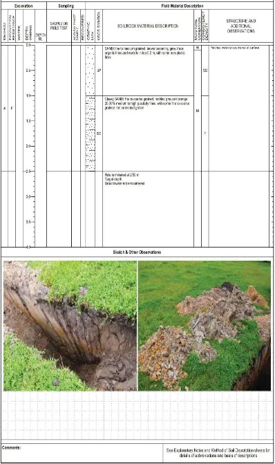
[image:17.595.134.462.182.615.2]Hydraulic conductivity or permeability of a soil is the most significant soil parameter influencing subsurface drainage design. (Hillman and Cocks 2007), advise that the hydraulic conductivity of sand in the Perth area varies as a result of fines content, which is defined as the percentage fines less than 0.075 mm particle size. Values vary from less than 1 m/d to 10 m/d. Figure 4 shows a typical PSD for imported fill sand used in the Dunsborough region.
Figure 4 – Typical Particle Size Distribution for Fill Sand in the Dunsborough Region. (Calibre Consulting (Aust) Pty Ltd)
Page | 8 Table 1 – Indicative saturated hydraulic conductivity values for various soil mediums (UNSW 2007)
2.7
Specific Yield
Specific yield is another soil property that is significant when considering subsurface flow. Hillman Cocks 2007 define this as the “amount of water released as the sand is drained, measured as a proportion by volume, or conversely the amount required to fully saturate the soil”. When the soil profile is free draining, a percentage of water is held due to capillary forces which means that the specific yield is less than the porosity as the pore space is partially filled with water. A figure of greater than 0.2 but less than 0.25 is indicative imported fill sands (Davidson, 1995).
2.8
Steady State Flow
[image:18.595.133.461.71.292.2](Leach and Volker 2005) summarise steady state flow as, a flow that occurs when, the magnitude and direction of the flow at any point in an area of analysis are constant with time. Steady State flow produces a curved surface as shown in the diagram below. The maximum mounding generally occurs at the midpoint between subsoil drains except when concentrated recharge occurs that may cause localised mounding.
Figure 5 – Typical mounding under steady state conditions: Drainage Principles and Applications (Ritzema HP 1994)
Page | 9 Isotropic and as such there would be no variance in hydraulic conductivity throughout the soil profile.
2.9
Unsteady or Transient Flow
Transient flow occurs when recharge rates, or infiltration varies with time. Transient flow is common and equations representing this type of flow are regularly used in software packages to calculate subsurface flow for use in engineering situations, infiltration problems and pump tests (Leach and Volker 2005).
2.10
Swan Coastal Plain Groundwater Environment
Barber 2005, reported that aquifers exist within the Aeolian sands and coastal limestone that exist on the Swan Coastal Plain. These aquifers are recharged by infiltration from rainfall. There are extensive swamps and wetlands that exist along the Swan Coastal Plain that rely on groundwater systems. Ephemeral streams exist on the eastern extremity of the plain into which groundwater also discharges as well as significant river systems like the Swan and Moore Rivers.
Mounding of the groundwater occurs across the plain due to recharge from rainfall infiltration, with the highest point of the mounding occurring centrally, then tapering off to the discharge points in the east and west. The phreatic surface breaks to the surface in some locations due to the undulating shape of the natural surface. These are the locations at which swamps, wetlands and damp lands have formed, with the size and depth of these features fluctuating with groundwater rise and fall. In areas of urban development and horticultural land uses many of these waterbodies have become eutrophic. Management strategies including artificial recharge, groundwater use limitations, groundwater monitoring and modelling have all been employed with varying degrees of success, however they have not prevented a decline in groundwater levels at a steady rate since the 1950s. In extreme cases some wetlands no longer exist (Barber 2005).
2.11
Dwellings, Buildings, Development Issues
2.11.1
An Overview of Western Australian Drainage Design
Principles
In Western Australia, drainage design principles are generally developed and enforced by the various local governments and the Department of Water. In general, small 1 year 1hr events are captured and soaked in bio-retention systems located at source within road reserves. These are designed in accordance with “Water Sensitive Urban Design”
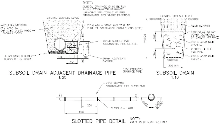
Page | 10 Figure 6 – Typical Subsoil Details (Calibre Consulting (Aust) 2016)
For residential developments there is generally two alternatives for the onsite treatment of stormwater for individual lots. Generalised figures showing these are shown below.
Figure 7 – Typical Residential Onsite Drainage Systems
[image:20.595.103.354.346.686.2]Page | 11 soak wells per lot is determined by the overall drainage design but in general they are normally sized to cater for a portion of the 1 in 5-year event with the remainder of the storm event accounted for in the street drainage design. There are pros and cons to this method of onsite stormwater disposal.
Pros: Stormwater is recharged to the groundwater profile at or close to the source of the rainfall. It is a tried and true drainage system that requires little to no maintenance and its design is very simplistic and does not require professional expertise for maintenance or construction. It is also a standalone system that has no interconnection to the local government street drainage.
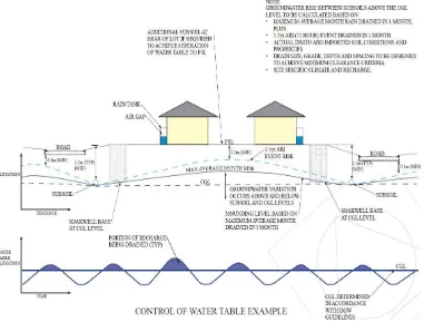
[image:21.595.102.483.305.594.2]Cons: Soak well disposal of stormwater results in a high level of water recharge to the soil profile. This causes increased groundwater mounding and as a result increased levels of fill to achieve the required separation distances. Subsoil drainage is also required to reduce the effect of mounding. Subsoil is generally placed in the street running parallel to street drainage but in some instances may also be required in the rear of properties as the shorter the separation between subsoil drains the less the mounding.
Figure 8 – Groundwater mounding requirement (Calibre Consulting (Aust) Pty Ltd)
The second option available for onsite treatment of stormwater is to install solid walled sub surface tanks (not perforated) that connect to the local government street drainage. These tanks do not allow soakage with their sole purpose being to store and detain flow. A throttled outlet is installed from the tanks to a connection point in the street drainage, this outlet is sized so that the tanks fill up during the peak storm event but do not over flow. There are also pros and cons to this method of stormwater disposal.
Page | 12 obvious economic benefit as well as an environmental benefit in the reduction of carting and extraction of sand fill.
Cons: It could be argued that transporting the stormwater away from the source via piped stormwater systems and disposing or soaking it at an end point location is interrupting the local cycle and movement of groundwater. There is also a direct interaction between the onsite disposal system and the local government street system which can cause
complications with maintenance responsibilities.
2.11.2
Relevant Legislation and Guidelines in Western
Australia
The land development industry in Western Australia has developed a series of accepted groundwater separation distances and guidelines through individual’s experience and general industry discussion. The “IPWEA Draft Specification for Separation distances for groundwater controlled urban development” was developed to formulate these guidelines and provide a guide to engineers working within the industry. The following is a
summary of this guideline with detail removed that is not seen as relevant to this project. The objective of the groundwater separation distance guidelines, as described in the document, “is to provide criteria (specifications) for groundwater separations appropriate to acceptable levels of risk and amenity for critical elements of built form and
infrastructure and provide guidance regarding appropriate methodology (design) for assessment and approval of groundwater levels and separations” (IPWEA 2016). When designing subsurface infrastructure, modelling is required to ensure that drainage systems will be sufficient for their purpose. Generally, when assessing subdivisions and their subsurface drainage requirements, analysis will be conducted on several typical locations within the development. This would include a section through a typical back to back lot configuration and potentially any recreational areas where drainage and
groundwater mounding may be an issue.
The design of groundwater systems is integral to the performance of: Roads and service infrastructure.
Earthworks design.
Landscape elements including public open space and water quality treatment systems.
Page | 13 Table 2 – Summary of groundwater modelling requirements – Draft Specification distances for groundwater-controlled urban development (IPWEA 2016 p4)
2.11.2.1
Models
The IPWEA document gives guidance on model selection for various tasks.
A selection of modelling methodologies are currently used by the industry. The various model types which the document considers appropriate are:
• Steady state calculations which are typically spreadsheet based.
• Dynamic models which can be spreadsheet based or developed within software packages.
2.11.2.2
Boundary/Initial Conditions
The IPWEA guideline summarises the use of boundary conditions and what is deemed appropriate for design.
Page | 14 the drain discharge capacity. In areas where no subsoil drainage exists it is suggested that a worst case groundwater level at the boundary may need to be considered.
For two dimensional or three dimensional models fixed or variable boundary conditions should be established using regional or district scale modelling and or, if available, groundwater monitoring data meeting the requirements of the Australian groundwater modelling guidelines (Sinclair Knight Merz).
2.11.2.3
Geotechnical and Hydrological Parameters
(IPWEA 2016) defines the following parameters to be applied when undertaking design calculations:
• Specific yield for imported fill = 0.2 • Hydraulic conductivity for imported fill = 5 m/day
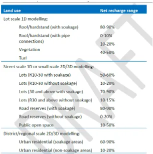
[image:24.595.145.451.301.609.2]The guideline also proposes recommended net recharge ranges for different scales of groundwater investigation. See Table 3 below.
Table 3 – IPWEA recommended groundwater recharge rates - Draft Specification distances for groundwater-controlled urban development (IPWEA 2016 p7)
A typical back to back lot cross section is assumed for the ranges shown in table 3, these are made up of portioned recharges from different surfaces as detailed below:
Hardstand = 0% recharge
Street soakage = 90% recharge
Turf = 50% recharge
Mixed turf/vegetation = 30% recharge
Page | 15 These recharge rates are combined to give a proportioned rate to be used for uniform recharge. The recommended values are
Small backyards with soak wells = 80% recharge based on a ratio of 100% for roof/hardstand and 50% for turf.
Large backyards with soak wells = 60% recharge based on a ratio of 100% for roof/hardstand and 50% for turf and gardens.
It was noted that there was no specific detail given in the guideline for what constitutes a “small backyard” or a “large backyard” assumptions would have to be made by the reader to categorise various sites.
2.11.2.4
Separation Distances
The following tables detail “deemed to comply” separation distances for various land uses as outlined in the IPWEA guide. These will be used for further analysis in this project.
Table 4 – Drainage infrastructure separation distance - Draft Specification distances for groundwater-controlled urban development (IPWEA 2016 p10)
Page | 16 Table 6 – Turfed Public open space separation distance based on typical soil types - Draft Specification distances for groundwater-controlled urban development (IPWEA 2016 p11)
The guideline’s generalised approach to subsurface drainage design is to select an appropriate model, calculate the phreatic surface and then add the deemed to comply separation distance to achieve a finished earthwork level. It’s worth noting from the figure below that the capillary fringe is not included in the separation distance. This is likely due to the time that capillary effects take place being a lot longer than the time a groundwater mound returns to a normal state after a storm event.
Page | 17
3.0
Steady State Equations
3.1
Darcy’s Law
In 1856 a French engineer named Henry Darcy published a report that described his study of the flow of water through a sand medium (Leach & Volker 2005). Darcy performed an experiment that measured the head and rate of flow. He observed that that the rate of water flowing through a sand profile per unit of time had a relationship to the difference in head of the water levels from one end of the sample to the other and to the length that the water had to flow.
The result of these findings is known as Darcy’s Law and is described in the equation below:
Q = -KA𝛥ℎ 𝛥𝑙
Where:
Q = Discharge measure in units of volume per time (m3/s); K = hydraulic conductivity distance per time (m/s);
𝛥ℎ
𝛥𝑙= hydraulic gradient;
A = cross sectional area, units of area (m2).
Darcy’s Law assumes slow laminar groundwater flow, which is the case in the majority of situations. Ritzema 1994, defines laminar flow in terms of Reynolds number and indicates that a value equal to or less than 1 will allow the use of the Darcy equation. The equation for Reynolds number:
Re = v x d50 x ρ 𝜂
Where:
v = Apparent velocity or discharge per unit area (m/s) d50 = mean diameter of soil grain (m);
p = mass density (kg/m3); and n = dynamic viscosity (kg/ms).
In general, Darcy’s Law can be used for saturated flow, steady state flow, unsteady or transient flow. It can be used in homogeneous materials and heterogeneous materials, isotropic and anisotropic situations (Leach & Volker 2005).
3.2
Dupuit Theory
Page | 18
𝑣 = −𝐾(𝑑𝑦
𝑑𝑥)T
The equation for the hydraulic gradient between two points is: S = (𝑑𝑦
𝑑𝑥)
These assumptions can under estimate the water surface in the vicinity of subsoil drains given the steep slope of the surface water in these locations (Ritzema 1994).
3.3
Darcy’s Law Hillman and Cocks Application
M.O. Hillman and G.C. Cocks are two engineers that were employed by Coffey Geotechnics Pty Ltd. They prepared a paper titled “Subsoil Drainage Design – Perth Residential and Road Developments” that was published in Australian Geomechanics Vol 42 No 120 on the 3rd of September 2007. The method of subsoil drainage design detailed in this paper is based on Darcy’s Law and the Hooghoudt equation. The following is a summary of the Hillman Cocks paper.
(Hillman and Cocks 2007) summarised that the important aspects to subsoil drain design in Perth sand environments are:
1. Thickness of sand layer overlying an impermeable layer and
2. The degree of groundwater mounding above the impermeable layer.
(Hillman and Cocks 2007) suggested that the time frame required to see a rise in water table due to capillary action is weeks and potentially longer. When a soil profile is subject to recharge from rainfall infiltration or stormwater recharge the phreatic surface will rise as water moves through the sand to subsoil drains, capillary rise associated with this new level could take a lot longer to achieve a significant rise than it will take the subsoil drains to drain the recharged water and reduce the water table to the previous level. Thus it is the reader’s interpretation that capillary rise can be neglected in the calculation of mounding within sand fill layers. This supports the IPWEA paper where the capillary fringe is neglected in the separation requirements.
The typical scenario discussed in the paper and as detailed in previous sections of this report involves parallel drains that intercept groundwater and control the level of the phreatic surface between the drains. Groundwater fluctuates due to rainfall infiltration from the surface and stormwater discharge from concentrated sources such as soak wells. The model assumes steady state conditions and a soil profile consisting of sand over an underlying impermeable layer.
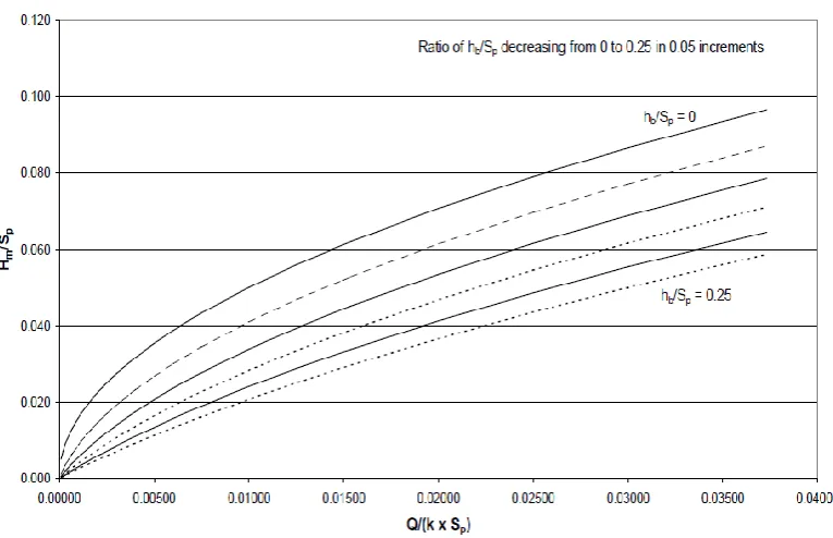
As detailed in figure 10 the height (Hm) of the mound is a function of the distance between the subsoil drain and the midpoint of the mound which is defined as (Sp). Other inputs required are the hydraulic conductivity of the sand layer, and recharge to the water table that occurs within section being analysed (Hillman & Cocks 2007).
Hm = Height of the mound at the midpoint between drains. (m) Sp = The distance from a drain to the midpoint. (m)
Hb = the level of subsoil drainage above the impermeable layer (m) K = Hydraulic Conductivity (m/day)
Page | 19 Figure 10 – Hillman Cocks Method
(Hillman and Cocks 2007) reported that Darcy’s Law can be used to calculate the height (Hm) under assumed conditions, and listed the assumptions as:
The hydraulic gradient varies from crest of mound to drain invert.
Distributed infiltration from rainfall will start flowing toward the drain locations at a flow rate increasing from 0 at the mound to its maximum at the drain. The method described the integration of the Darcy equation for ΔHm / ΔSp, resulting in two sets of equations as listed below:
Uniformly Distributed Rainfall
Concentrated Infiltration (at crest of mound)
These equations were then used to develop the figures below.
Page | 20 Figure 12 – Concentrated infiltration at crest of mound (Hillman & Cocks 2007)
A combination of the two conditions represented in the figures would commonly occur in land development where soak wells are regularly used for onsite stormwater disposal. Hillman and Cocks suggest that judgement needs to be made about the type of
distribution of rainfall within the section being analysed. The two charts can be used to assess a range or limits of the mound height based on a given recharge to the section being analysed. When using the charts engineering judgement needs to be used to assess the degree of uniform and concentrated flow for the site.
An approximate estimate of the height of the phreatic surface at any point between the drain and the mound is given by:
A = 0.175 ln B + 1 (3) for the uniformly distributed case. A = 0.4 + 0.6 B (4) for concentrated infiltration.
A = ratio of height at point of interest, to total mound height.
B = ratio of distance from drain at point of interest to distance to crest of mound. When applying the above method to residential lots the (Hillman & Cocks 2007) summarised method is given below.
A rainfall should be selected that represents an event most suitable for design. The rainfall intensity selected should be factored to give the actual recharge or
infiltration rate;
Refer to the design charts to assess upper and lower values of the height of mounding.
3.4
Hooghoudt Equation
Page | 21 The Dupuit-Forchheimer theory is based on the principle that Darcy’s formula can be used to calculate flow through a vertical plane at a selected distance from subsoil drainage. Considering this plane at the subsoil drain location the continuity principle is true when the water that enters the soil profile in the area between the plane and the midpoint of the subsoil drains passes through the vertical plane to enter the drain (Ritzema 1994).
The Hooghoudt Equation shown below was developed based on these principles. q=8𝐾𝑑ℎ+4 𝐾ℎ2
𝐿2 Where:
q = drain discharge (m/d)
K = hydraulic conductivity (m/d); d = equivalent depth (m)
L = spacing between drains (m)
h = height of mounding above the drain (m).
Hooghoudt developed the concept of an imaginary impervious layer that relates to an equivalent depth. When drains are positioned above the impervious layer, extra head loss is required to achieve the same flow rate in the drains. The equivalent depth accounts for this head loss.
The equivalent depth d was further developed by (Van der Molin and Wesseling 1991) (As cited in Ritzema 1994) who developed formula for the exact calculation of d.
Where:
Two important assumption of the Hooghoudt equation are that: Flow is to a height of half the subsoil drains
Page | 22
4.0
Dynamic Model - Unsteady state
4.1
MODFLOW GMS (Aquaveo)
(Harbaugh, Banta, Hill and McDonald 2000), describe MODFLOW as a computer program that simulates three-dimensional groundwater flow through a porous medium by using a finite difference method. It uses a modular structure which groups programs of similar function together, options in the model are constructed so that they are
independent of each other. MODFLOW can be used to compute two or three dimensional models.
The below partial-differential equation describing the movement of groundwater is used in MODFLOW.
Where:
Kxx, Kyy, and Kzz represent hydraulic conductivity in the x, y, and z coordinates, which the model assumes are parallel to hydraulic conductivity major axes (L/T).
h = potentiometric head (L)
W = represents volumetric flux per unit volume from recharge sources i.e. rainfall infiltration, wells etc. (W<0.0 represents out flow and w>0.0 flow into system (T-1) Ss = the porous materials specific storage (L-1)
t = time (T).
Figure 13 - MODFLOW cells (U.S. Geological Survey)
The above equation is what is used to describe transient, three-dimensional groundwater flow once combined with initial and boundary conditions, and assumes a heterogeneous and anisotropic profile.
The equation above is solved using the finite element method. The software divides the groundwater flow system into a series of cells, as per Figure 13, and assigns each cell a node for which the head is calculated.
Page | 23 Where:
h = the head at each individual cell reference for a time step (m). CV, CR, CC = Hydraulic conductance’s between adjacent nodes.
P = the sum of coefficients of head for recharge terms for each cell reference.
Q = the constants from recharge terms summed for each individual cell. Q is negative for outflow from the system and positive for inflow.
SS = the specific storage for each cell. This is only relevant to transient simulations. DELR = the width of cells in the specific column.
DELC = the width of cells in the specific row.
Page | 24
5.0
Methodology
[image:34.595.101.496.507.741.2]As already discussed the theoretical analysis will be based on soil conditions, climate conditions and hydrogeological characteristics representative of Dunsborough in Western Australia. The drainage condition to be analysed will consist of a 2 layered soil profile made up of permeable sand fill over impermeable natural clays creating a perched water table. This design scenario is typical of that experienced in the Dunsborough region. The main objective is to compare the methodology and results associated with the calculation of the peak mounding of the phreatic surface within the permeable sand layer.
An analysis will be conducted using steady state models, which will be compared for variations and accuracy in calculating the degree of mounding. Transient models will then be used to analyse the site to provide a further comparison. Various stormwater disposal methods will also be analysed to assess which method provides the most efficient design in minimising the phreatic surface mounding.
The steady state models to be used in the analysis are: Darcy/Dupuit Equation
Hillman and Cocks method Hooghoudt Equation
MODFLOW
The Dynamic Model to be used in the analysis is:
MODFLOW
5.1
Collation of Site Specific Data
Below is a table that summarises the required inputs as listed in the literature and the values that will be used in the selected test case analysis. These values will be constant across all the analysis cases.
Value as suggested in Guidelines Value selected for Test case Remarks Hydraulic Conductivity (m/day)
1 – 10 5 This is industry accepted
value for typical imported fill sand compacted to 95% MMDD.
Separation Distance (mm)
300 300 As required by the IPWEA
Guideline. Subsoil Drain
spacing
30-40 when subsoil located at rear of lots. 60 – 90 road reserve to road reserve
35, 60 and 90
The intention is test all cases.
Rainfall recharge rates (%) uniformly distributed - soak wells
Page | 25 Rainfall recharge
rates (%) Uniformly distributed - No soakage, connected to street drainage.
10% -20% 20% This is based on the area
of the lot and proportion of hardstand and vegetated surfaces.
Rainfall recharge rates for detailed lot analysis (%)
Turf Areas 50% Hardstand Areas 90%
50% 90%
Rainfall Event 1 in 2 yr 72hr event 1 in 2 yr 72hr event Rainfall Intensity
(mm/hr)
[image:35.595.99.496.360.668.2]- 1.21 As provided by the Bureau of Meteorology
Table 7 – Standard IPWEA Requirements relevant to the Analysis.
5.2
Model Development
5.2.1
Hooghoudt Equation
A spreadsheet was prepared that calculates the maximum mounding based on the Hooghoudt equation using the required inputs. A graph displaying the distribution of mounding between the subsoil drain and the maximum mounding height was included.
Figure 14 – Steady State Flow Spreadsheet Hooghoudt Equation
5.2.2
Hillman Cocks Method
A spreadsheet was prepared based on the calculations required for the Hillman Cocks method. The two cases for concentrated flow and uniformly distributed flow are
calculated separately and then a ratio is applied to achieve the final calculated mounding height. The ratio applied in this theoretical model is based on the proportion of hardstand
Hooghoudt Equation
Project: x (m) h (m)
0 45 0.05
Input Data 5 40 0.89
10 35 1.25
Insitu Soil Permeability (m/day) K 5 15 30 1.53
1:2yr 72 hr event (mm/hr) 1.21 20 25 1.77
Recharge (%) 60 25 20 1.98
Depth to impermeable layer below subsoils (m) d 0 30 15 2.17
Drain Spacing (m) L 90 35 10 2.34
40 5 2.50 1:2yr 72 hr event total rain (mm) 87.12 45 0 2.66 Total design recharge rate (m/d) q 0.0174
a= 4K= 20
b= 8KD= 0
c= -QL2 -141.13
maximum rise between subsoils (m) h 2.66
0.00 0.50 1.00 1.50 2.00 2.50 3.00
0 10 20 30 40 50
Page | 26 area to lawns and gardens as the hardstand area is assumed to be directed to soak wells, which is concentrated flow, and lawns/gardens uniformly distributed flow. The hardstand to lawn/garden ratio is calculated for each test case based on the lot size and assuming a constant house area for all test cases. A graph showing the distribution of the mound over the distance between the subsoil drain and the midpoint has been included. This is calculated using the Hillman Cocks recommended method. It should be noted that in this method the discharge q = the recharge rate and this is represented in (m3/day).
Figure 15 – Steady State Flow Spreadsheet Hillman Cocks Method
5.2.3
Darcy/Dupuit Equation
(Fetter 2001) detailed that a combination of the Darcy Equation, Q = -KA𝛥ℎ
𝛥𝑙, and the Dupuit Equation q’ = 1
2𝐾( ℎ12−ℎ22
𝐿 ), can be derived to produce the equation below:
ℎ = √ℎ12−(ℎ1
2− ℎ22)𝑥
𝐿 +
𝑤
𝑘(𝐿 − 𝑥)𝑥
Where:
h = the head at a distance x (m).
x = the distance from the subsoil drain (m).
h1 = the head at the origin point (m). In this instance h1 is at the subsoil drain. The drain is assumed to be a diameter of 150mm and flowing half full, so h1 has a value equal to 0.075m.
Hillman Cox
x(m) B A Hm (Uniform) A Hm (Concentrated) Hm (factored) Sp (m) 45 Distance from drain to midpoint 0 0.05
hb (m) 0 Distance of drain above impervious 5 0.111111 0.615486 1.633879795 0.4666667 1.751958904 1.687015394
Q (m3/d) 0.783 0.0174 10 0.222222 0.736786 1.955887041 0.5333333 2.002238747 1.976745309
K(m/d) 5 15 0.333333 0.807743 2.144249206 0.6 2.25251859 2.192970429 20 0.444444 0.858087 2.277894288 0.6666667 2.502798434 2.379101154
Uniform Hm (m) 2.654619 Max HM 3.149429 25 0.555556 0.897137 2.381557468 0.7333333 2.753078277 2.548741832
Concentracted Hm (m) 3.754198 30 0.666667 0.929044 2.466256452 0.8 3.003358121 2.707952203 35 0.777778 0.95602 2.537868424 0.8666667 3.253637964 2.859964717 40 0.888889 0.979388 2.599901535 0.9333333 3.503917807 3.006708857 45 1 1 2.654618617 1 3.754197651 3.149429182
0 0.5 1 1.5 2 2.5 3 3.5
0 5 10 15 20 25 30 35 40 45
Page | 27 h2 = the head at L (m). When calculating the maximum mound at the midpoint this value is also 0.075m as it represents the second subsoil pipe and L represents the spacing between the two pipes.
K = the hydraulic conductivity of the soil (m/d) w = the recharge rate (m/d).
This equation is valid for steady state flow and is based on the principle that any change of flow is equal to a change in the water table. In this instance the change is a gain and is due to stormwater infiltration. This infiltration is represented by w (recharge rate). The equation calculates the elevation h of any point between h1 and h2 allowing for a recharge between h1 and h2.
[image:37.595.99.490.292.539.2]A spreadsheet was developed using this formula to calculate the maximum (h) given the required inputs. This equation was also used to develop a graph showing the variance in the mound between the subsoil drainage and the crest of the mound.
Figure 16 – Steady State Flow Spreadsheet Darcy/Dupuit Equation
5.2.4
MODFLOW – Steady State
Steady state analysis in MODFLOW works on the principle that all flows entering and exiting the individual cells sum to zero at the end of the simulation. Steady state
simulations utilize a single stress period and exclude any storage effects within the cells. MODFLOW utilizes a backwards difference approach in solving the finite difference equation for steady state flow. The equation used for steady state solutions is the same as used for transient solutions with the storage terms removed.
For the steady state analysis, a grid approach was adopted as this method is best suited to small scale scenarios. A grid 100m long by 40m wide and 3m deep was created to represent 4 residential lots in a back to back configuration as shown in figure 17. Darcy Dupuit Formula
x(m) h (m) h1 (m) (head at origin) 0.075 0 0.05
h2 (m) (head at L) 0.075 5 1.219391
L (m) 90 10 1.671534
K (m/d) 5 15 1.981641
2yr 72hr event (mm/hr) 1.21 20 2.210324
Recharge Rate (%) 60 25 2.38116
w recharge (m/d) 0.017424 30 2.506008 35 2.591523
h max (m) 2.6575073 40 2.641527 45 2.658025
0 0.5 1 1.5 2 2.5 3
0 5 10 15 20 25 30 35 40 45
Page | 28 Figure 17 – XY Grid Layout MODFLOW
This three-dimensional box was then divided into 1m x 1m x 1m cells. The bottom of the box represents the clay layer as an impermeable surface with zero hydraulic conductivity. Each cell was assigned a hydraulic conductivity of 5m/day as per the recommended guidelines. This value was the same in both the vertical and horizontal directions to replicate a homogenous soil type.
The optional “Drains” package was utilized to replicate the slotted subsoil drains running parallel within the road reserves. MODFLOW applies a drain function on a cell by cell basis. A row of cells on either side of the grid at the bottom layer were converted to drain cells. These drain points are applied central to the cell with an elevation of 0.05 to simulate a drain laid just above the impermeable surface. MODFLOW requires a conductance to be specified for the drainage cells, for the purpose of this analysis it is assumed that the drains would be suitably designed to handle the subsurface flow rates so that the controlling factor influencing mounding will be the hydraulic conductivity of the soil and not the capacity of the subsoil drains. As such, a high value of conductance was applied to the drainage cells of 1000 m2/d.
The solver package selected for the analysis was the Preconditioned Conjugate-Gradient Package. This package utilizes inner and outer iterations that must be user defined. For all the analyses conducted iterations of 50 and 100 for inner and outer were selected
respectively. The wetting of cells option was enabled which allows for the calculation of the variance in head between when the cell is wet and dry.
The “Recharge” package was used to simulate rainfall recharge to the soil profile. This package was configured so that recharge was applied at the “highest active cell in the model”.
These basic setup configurations remained constant for all the scenarios that were modelled.
5.2.5
MODFLOW – Transient
Page | 29 The mean annual rainfall for Dunsborough as listed on the Bureau of Meteorology
website is 805.3mm. The rainfall experienced in the year 2000 was chosen for the analysis, as this year had a total rainfall 881.2mm which is slightly above the mean rainfall value and so was seen to be conservative. This year contains 5 daily rainfalls equal to or above the steady state modelled rainfall of 29mm per day.
Page | 30
6.0
Analysis
6.1
Theoretical Test Case One (90m Separation)
The first case to be analysed will be a typical back to back lot configuration with a separation of 90m between subsoils. The site is assumed to consist of natural clay soils with no or very low permeability. Fill is required over the site to achieve site
classification and to allow for disposal of stormwater through soak wells. Subsoil drainage will be placed in the street verge at the natural clay level. The theoretical site will consist of lots 40m deep giving a separation of 90m between subsoil drains when allowing for a 5m alignment of the drain within the road reserve. The remaining inputs are:
Rainfall intensity – 121mm/hr Recharge rate – 60%
Recharge to water table (m/d) – 121 x 72/3 x 0.6 = 0.0174m/d Recharge to water table (m3/d) – 0.0174 x 45 = 0.783 m3/d L = 90m
K = 5m/d
The purpose of this first analysis is to compare the steady state methods against a transient model. With the exception of the Hillman and Cocks model a uniform distribution of recharge across the lots will be assumed.
6.1.1
Results
Below is a graph showing the groundwater mounding height as calculated by the four steady state models and the MODFLOW transient model.
Figure 18 – Theoretical Case 1 Comparison
There are two obvious trends that can be seen in the graph. The Hooghoudt and Hillman Cocks results are relatively parallel with the Hillman Cocks values being slightly higher by a consistent value of approximately 0.5m. This can be attributed to the Hillman Cocks method’s allowance for concentrated flow. The concentrated flow equation multiplies the flow rate by a multiple of 2. Although it is not clearly documented this appears to be an
0 0.5 1 1.5 2 2.5 3 3.5
0 10 20 30 40 50
G ro u n d w at er m o u n d in g (m )
Distance from Subsoil Drain (m)
Theoretical Case 1 Comparison
Page | 31 allowance for 2 soak well systems, one for each lot (back to back) applied at the midpoint or close to the maximum mounding height.
The second trend can be seen in the comparison between the Darcy/Dupuit and
MODFLOW calculations. The results calculated by these two models run parallel in the graph with the MODFLOW results consistently higher by a value of approximately 0.3m. The MODFLOW literature documents that the MODFLOW programme utilises the principles of Darcy’s equation to calculate the flow, or specifically the conductance from one cell to another, so it seems reasonable that the two sets of results would be
comparable. The variance between the two models could be attributed to MODFLOW’s ability to calculate a head variance for individual cells between when they are wet and dry.
The Darcy/Dupuit and Hooghoudt models both converge to the same maximum mounding height while the Hillman Cocks model has the closest result to the MODFLOW software model.
Both the Hooghoudt and Hillman Cocks models have a relatively steep, almost linear, distribution of the groundwater mound between the maximum height and the end of the model at 5m. When reviewing the literature for the two methods, both utilise the recharge rate in calculating the maximum recharge height but ignore this value when calculating the distribution of mounding with (x) distance from the subsoil drain. The other methods consider the recharge when calculating the mound distribution for (x) and as a result have a significantly more curved distribution.
The results for the transient analysis are significantly lower than all of the steady state analysis. The maximum mounding occurs on September the 7th in response to a rainfall event of 62mm, this occurred after 6 consecutive wet days including 4 days where over 10mm of rainfall was recorded. Of the 16 days prior to the maximum mound 13 experienced rainfall. From this data it can be surmised that the maximum mounding occurred on this day due to a long period of inundation plus a significant rainfall event of 62mm recharging the soil profile.
In practice construction sites will have anywhere between 1.0m to 1.5m of sand fill. Through years of application this range of fill has been proven to handle fluctuations in groundwater mounding adequately. Considering this range as a bench mark, the results produced by the transient method are reasonable whereas the steady state results appear to be conservative. A table is shown below listing all of the maximum values and their percentage variance to the transient solution as a comparison.
Method
Maximum Mounding
(m)
% variance to Transient
Model
Hooghoudt 2.66 116%
Hillman Cocks 3.15 156%
Darcy/Dupuit 2.66 116%
MODFLOW 2.95 140%
MODFLOW Transient 1.23 0%
Page | 32
6.2
Theoretical Test Case Two (90m Separation Soak wells at
Rear)
With the exception of the Hillman Cocks model the analysis in case 1 assumes uniform recharge of rainfall to the soil profile. However, in a residential context this is unlikely to occur. In practice recharge from rainfall is collected by gutters and hardstand areas and then piped to soak wells, where recharge to the soil is then concentrated at specific locations. To try and simulate these concentrated conditions three additional simulations were run in MODFLOW.
The first simulation was setup to replicate soak wells being positioned at the rear of the property. A house area of 18 x 20 metres was assumed. The cells that represent the house had their recharge value set to zero. The standard requirement for the sizing of soak wells is to allow 1m3 per 65m2 of hardstand area. Based on an area of 360m2 the requirement would be 5.5m3 of soak well. For the analysis 6 cells per lot were used, being 1m3 per cell, 6m3 in total. The rainfall runoff from the hardstand area was added together and applied evenly to the 6 cells. As per the IPWEA guidelines a recharge factor of 90% was applied to the hardstand runoff and 50 % was applied to the remaining uniformly
distributed recharge through lawns and gardens. Steady State
29.04mm/day x 360 x 0.9 = 9408.96mm
9408.96/6 = 1568.16mm = 1.57m/day per soak well. Transient
As per steady state but calculated for each daily time steps rainfall Other inputs:
Rainfall Intensity – 121mm/hr Combined Recharge rate – 60% Hardstand Recharge rate – 90% Lawns/Gardens recharge rate – 50% Spreadsheets
Recharge to water table (m/d) – 121 x 72/3 x 0.6 = 0.0174m/d Recharge to water table (m3/d) – 0.0174 x 45 = 0.783 m3/d L = 90m
K = 5m/d
A figure showing the application of the recharge values for the soak wells at rear analysis is shown below. The green areas are cells with a uniform recharge rate, the red represents 0 recharge while the 6 purple cells per lot are the theoretical soak well locations.
Page | 33 Figure 19 – Distribution of Recharge
A model was also prepared for the situation that occurs when soak wells are installed at the front of the house. The model was prepared on the same principles as the rear of the house simulation but with the six soak wells located within the front 6m of the lot. The figure below shows the distribution of head for this simulation, note the wave or mounded distribution around the soak well locations.
Figure 20 – Head distribution for soak wells located at the front of lot.
Page | 34 Figure 21 – Head distribution for soak wells located at the rear of lot
6.2.1
Results
The graph below represents the results of theoretical case one overlayed with the rear and front soak well simulations.
Figure 22 – Theoretical Case 2 Comparison
When considering the above results, the soak wells at rear results obtained from the MODFLOW steady state analysis are significantly higher than all other results. Applying a recharge of 1.57m per day in a steady state analysis appears to give a very conservative result with little design value for engineers when compared with the other methods. This degree of mounding is well in excess of what is seen in practice in Dunsborough. As previously stated the Hillman Cocks method allows for concentrated flow from soak wells by applying a factor of 2 to the flow, the maximum mounding is slightly higher at
0 1 2 3 4 5 6
0 5 10 15 20 25 30 35 40 45
G
ro
u
n
d
w
at
er
m
o
u
n
d
in
g (m
)
Distance from Subsoil Drain (m)
Theoretical Case 2 Comparison
Hooghoudt
Hillman Cocks
Darcy/Dupuit
Modflow (Uniform Distribution)
Modflow (Soak wells at Rear)
Modflow (Soak wells at Front)
Modflow (Transient)
Page | 35 the midpoint when compared with the other steady state methods, but the result converges to the MODFLOW uniformly distributed results quickly.
Between distance 10 and 30 the soak wells at rear results graph becomes linear for all three of the additional analysis in this test case. This represents the section beneath the house where the recharge is 0.
When comparing the uniformly distributed transient model to the soak wells at rear transient model, the latter has a higher maximum mounding value at the midpoint as would be expected. The soak wells at rear simulation then dips below the uniformly distributed simulation, this can be attributed to the 0 recharge beneath the house causing the curve to drop off steeply. When comparing the steady state simulations of
MODFLOW uniformly distributed and Hillman Cocks a similar pattern can be seen. The Hillman Cocks method is higher at the midpoint which is expected given its allowance for concentrated flow and then dips below the uniformly distributed curve.
As would be expected the soak wells at front results show a spike in the graph at distance 10m. Again it can be seen that there is a linear distribution for the area under the house where there is 0 recharge, although this section between 20 and 35 has moved further toward the rear of the block due to the additional recharge at the front of the block. Due to the uniform distribution of recharge in the rear of the theoretical lot the maximum
mounding matches the MODFLOW uniformly distributed result exactly. For this theoretical case the steady state equations are again significantly more
conservative than the transient models with the MODFLOW soak wells at rear simulation giving an extreme result. The Hillman Cocks method however appears to give a good steady state representation of concentrated flow with soak wells at or close to the midpoint when compared to the MODFLOW analysis ignoring its conservatism to the transient models.
The table below lists the maximum mounding heights for all of the models.
Method
Maximum Mounding (m)
Hooghoudt 2.66
Hillman Cocks 3.16
Darcy/Dupuit 2.66
MODFLOW 2.95
MODFLOW (Soak wells at
Rear) 5.27
MODFLOW (Soak wells at
Front) 2.95
MODFLOW Transient 1.23
MODFLOW (Transient
Soak wells at Rear) 1.59
Page | 36
6.3
Theoretical Test Case 3 and 4 (60m, 35m Separations)
The next set of analysis was run to test the sensitivity of distance between subsoil drains on mounding height between the various methods. In addition to the simulation modelled in theoretical test case 1, two additional sets of simulations were undertaken for a 60m drain spacing and a 35m drain spacing. The 35m spacing model best represents the onsite situation where a subsoil line would run parallel to the subsoil in the road verge but located at the rear of the property. The same rainfall intensities and methodology for applying discharge to soak wells was used as per the previous analysis. The theoretical house floor area is assumed to remain the same (360m2) while the length of the property is reduced. This will mean that the backyard areas will be reduced and intern the
uniformly distributed portion of the rainfall recharge will also be reduced. Inputs:
Rainfall Intensity – 121mm/hr Combined Recharge rate – 60% Hardstand Recharge rate – 90% Lawns/Gardens recharge rate – 50%
Recharge to water table (m/d) – 121 x 72/3 x 0.6 = 0.0174m/d Recharge to water table (m3/d) – 0.0174 x 45 = 0.783 m3/d L = 60m, 35m
K = 5m/d
6.3.1
Results Test Case 3
[image:46.595.100.498.503.732.2]Below is a graph showing the groundwater mounding height as calculated by the four steady state models and the MODFLOW transient models simulating theoretical test case 3 with 60m subsoil drain separation.
Figure 23 – Theoretical Case 3 – 60m Comparison 0 0.5 1 1.5 2 2.5
0 10 20 30 40
G ro u n d w at er m o u n d in g (m )
Distance from Subsoil Drain (m)
Theoretical Case 3 - 60m Separation
Hooghoudt Hillman Cocks Darcy/Dupuit Modflow (Uniform Distribution) Modflow (Transient)
Page | 37 From the graph above it can be seen that the Hillman Cocks method produces the highest maximum mounding compared with the other methods, this is consistent with the other two theoretical test cases. The MODFLOW uniformly distributed results compared with the Darcy/Dupuit results are again almost parallel. The Darcy/Dupuit and Hooghoudt equations result in the same maximum mounding value. The results produced by the MODFLOW transient simulation are significantly less than the steady state values, and the curve or rate of change in mounding is significantly less pronounced. The similarity in pattern between the two transient simulations and the MODFLOW uniformly distributed and Hillman Cocks method is again evident.
The maximum mounding values for the 90m and 60 transient soak wells at rear simulations are 1.59 and 1.37m respectively, while the 90m and 60m uniformly distributed values are 1.23m and 0.86m respectively. The variation in maximum
mounding height between the uniformly distributed transient model and the soak wells at rear transient model is 510mm, when compared to the previous test case variance of 360mm this is a significant increase. This is largely due to the concentrated flow rate remaining the same for both simulations while the uniformly distributed flow reduces, i.e. the house size remains the same regardless of the block size but the lawn/garden area reduces. This is a true representation of what happens in reality, as house sizes generally remain constant regardless of lot size.
With the exception of the transient models, in general, it could be said that the same patterns and similarities evident in the previous two test cases are again evident here. Perhaps the only slight variance is the difference in values at the 5m chainage for the MODFLOW uniformly distributed and Hillman Cocks results. The Hillman Cocks value is significantly less in this simulation compared with the previous and may indicate that the results obtained using this method are sensitive at or near the subsoil drain location.
6.3.2
Results Test Case 4
Below is a graph showing the groundwater mounding height as calculated by the four steady state models and the MODFLOW transient models simulating theoretical test case 4 with 35m subsoil drain separation. This theoretical test case has been created so that the subsoil drain is located on the rear boundary of the back to back lots as well as a subsoil drain in the street to give the 35m separation. For the steady state simulations replicating soak wells at the rear of the lots, this will mean that the subsoil drain is directly adjacent to the soak well locations. Because of this the steady state model for soak wells at the rear of the lot has been re-included into the set of simulations to see if this has an effect on its previous excessively conservative results.
Inputs:
Rainfall Intensity – 121mm/hr Combined Recharge rate – 60% Hardstand Recharge rate – 90% Lawns/Gardens recharge rate – 50%
Page | 38 K = 5m/d
Figure 24 – Theoretical Case 4 – 35m Comparison
From the graph above it can be seen that the steady state MODFLOW soak wells at rear method again produces the highest maximum mounding and has the highest distribution of mounding compared with the other methods. The graph has been extended for the full 35m between subsoil drains. This is to show that the maximum mounding location for the two soak well at rear simulations has moved to the rear of the lots from the midpoint between drains location. The MODFLOW uniformly distributed results compared with the Darcy/Dupuit results are again relatively parallel. The Darcy/Dupuit and Hooghoudt equations result in the same maximum mounding value, which is consistent with the previous theoretical case studies. The results produced by the two MODFLOW transient simulations are significantly less than the steady state values, and the curve or rate of change in mounding is significantly less pronounced.
The MODFLOW transient soak well at rear results show a dip at the midpoint between drains, this represents the area under the theoretical house where the recharge rate is 0. The mounding either side of this midpoint is due to point recharge at the soak well locations and uniformly distributed recharge in the theoretical front yards of the properties. The mounding due to the soak well recharge drops off severely as would be expected given that the subsoil drain is directly adjacent. When comparing the two transient models, although the mounding values at the midpoint are considerably different the maximum mounding values are similar, 0.57m for the uniformly distributed model, 0.54m for the soak wells at rear model, a 30mm difference, significantly less than the 510mm difference in these results in test case 3. It should also be noted that the soak wells at rear model is now less than the uniformly distributed due to the concentrated recharge location being directly adjacent to the subsoil drain.
In general, by introducing a subsoil drain at the rear boundaries of the theoretical lots the maximum mounding height across all the models has been significantly reduced.
Comparing the results of test theoretical test cases 1, 3 and 4 the results for the MODFLOW, Darcy/Dupuit, Hooghoudt and MODFLOW transient model follow a
0 0.2 0.4 0.6 0.8 1 1.2 1.4 1.6 0
2.5 5 7.5 10 12.5 15 17.5 20 22.5 25 27.5 30 32.5 35
G ro u n d w at er m o u n d in g (m )
Distance from Subs