Drought forecasting in eastern Australia using multivariate adaptive regression spline, least square support vector machine and M5Tree model
Ravinesh C Deo, Ozgur Kisi, Vijay P Singh
PII: S0169-8095(16)30450-1
DOI: doi:10.1016/j.atmosres.2016.10.004 Reference: ATMOS 3805
To appear in: Atmospheric Research Received date: 5 July 2016
Revised date: 4 October 2016 Accepted date: 10 October 2016
Please cite this article as: Deo, Ravinesh C, Kisi, Ozgur, Singh, Vijay P, Drought forecasting in eastern Australia using multivariate adaptive regression spline, least square support vector machine and M5Tree model, Atmospheric Research (2016), doi:10.1016/j.atmosres.2016.10.004
ACCEPTED MANUSCRIPT
Drought forecasting in eastern Australia using
multivariate adaptive regression spline, least square
support vector machine and M5Tree model
Ravinesh C Deo
1 *,Ozgur Kisi
2, Vijay P Singh
31
School of Agricultural Computational and Environmental Sciences International Centre of Applied Climate Sciences (ICACS) University of Southern Queensland, Springfield, AUSTRALIA
*Corresponding Author: [email protected]
2
Canik Basari University, Architecture and Engineering Faculty Civil Engineering Department, 55080 Samsun, TURKEY
3
Department of Biological and Agricultural Engineering and Zachry Department of Civil Engineering, Texas A&M University, 2117 TAMU, College Station, TX 77843-2117, USA
Abstract
Drought forecasting using standardized metrics of rainfall is a core task in hydrology and water resources management. Standardized Precipitation Index (SPI) is a rainfall-based metric that caters for different time-scales at which the drought occurs, and due to its standardization, is well-suited for forecasting drought at different periods in climatically diverse region. This study advances drought modelling using multivariate adaptive regression splines (MARS), least square support vector machine (LSSVM), and M5Tree models by forecasting SPI in eastern Australia. MARS model incorporated rainfall as mandatory predictor with month (periodicity), Southern Oscillation Index, Pacific Decadal Oscillation Index and Indian Ocean Dipole, ENSO Modoki and Nino 3.0, 3.4 and 4.0 data added gradually. The performance was evaluated with root mean square error (RMSE), mean absolute error (MAE), and coefficient of determination (r2). Best MARS model required different input combinations, where rainfall, sea surface temperature and periodicity were used for all stations, but ENSO Modoki and Pacific Decadal Oscillation indices were not required for Bathurst, Collarenebri and Yamba, and the Southern Oscillation Index was not required for Collarenebri. Inclusion of periodicity increased the r2 value by 0.5–8.1% and reduced RMSE by 3.0–178.5 %. Comparisons showed that MARS superseded the performance of the other counterparts for three out of five stations with lower MAE by 15.0–73.9% and 7.3– 42.2%, respectively. For the other stations, M5Tree was better than MARS/LSSVM with lower MAE by 13.8–13.4% and 25.7–52.2%, respectively, and for Bathurst, LSSVM yielded more
ACCEPTED MANUSCRIPT
MARS/M5Tree for Bathurst, Yamba and Peak Hill, whereas for Collarenebri and Barraba, M5Tree was better than LSSVM/MARS. Seasonal analysis revealed disparate results where MARS/M5Tree was better than LSSVM. The results highlight the importance of periodicity in drought forecasting and also ascertains that model accuracy scales with geographic/seasonal factors due to complexity of drought and its relationship with inputs and data attributes that can affect the evolution of drought events.
Keywords
Standardized precipitation index, drought forecasting, multivariate adaptive regression spline, least square support vector machine, M5 Tree model1.0 Introduction
Drought is an insidious natural hazard that occurs as a normal, yet a recurrent feature in an arid, semi-arid, desert or rain-forested region (Wilhite et al., 2000a; Keyantash and Dracup, 2002; Vicente-Serrano, 2016). Drought impacts are exacerbated by shifts to warmer and drier conditions, leading to increased water demand compounded by population growth and consequent expansion of industrial, agricultural and energy sectors (McAlpine et al., 2009; IPCC, 2012). As a critical environmental issue, challenges posed by drought elicit increased alertness among hydrologists, agriculturalists and resource planners in strategic decision-making (Bates et al., 2008; Mishra and Singh, 2011). Meteorological drought that transforms in a hydrological, agricultural and socio-economic events, onsets with a marked reduction in rainfall sufficient to trigger hydrometeorological imbalance for a prolonged period (Wilhite and Hayes, 1998; Mishra and Singh, 2010; Deo et al., 2016a). Drought is a costly hazard on socio-economic dimension, occurring on a year-to-year and season-to-season basis with detrimental outcomes due to its persistent effect on groundwater reservoirs, leading to water scarcity, crop failure, disturbed habitats and loss of social/recreational opportunities (Riebsame et al., 1991; Wilhite et al., 2000a; Mpelasoka et al., 2008). Effective strategies to forewarn drought are thus important for risk management.
ACCEPTED MANUSCRIPT
hydrological data (Stahl and van Lanen, 2014; Joaquín Andreu et al., 2015; Deo et al., 2016a). However, an understanding of future drought requires an evaluation of predictive models that are reliable enough to forewarn drought possibility (Mishra and Singh, 2011). Construction of a forewarning systems require action-oriented models that are implemented in a risk management program (Wilhite et al., 2000b; IPCC, 2007; Sheffield and Wood, 2008; Mishra and Singh, 2011).
Due to the complexity of drought that embeds localised, yet stochastic features and non-linearities between predictors and objective variable, modellers remain puzzled in adopting a model for all regions. Spiralling nature of drought makes it impossible to adopt a ‘one-size-fits-it-all’ so a deficiency in drought mitigation arises from inability to forecast the conditions well in advance (Mishra and Desai, 2005; Almedeij, 2015). Critical issues in drought modelling are: the inability to adopt a universal model, input selection, choice of index that sufficiently represents drought monitoring over different regions and the disproportionally areal and geographic impact that results in different model accuracy (Mishra and Desai, 2005; IPCC, 2012). In some regions, a model may not reflect the reality, thus, a rigorous testing of different models must be facilitated to establish a versatile framework that fits a prediction system. As drought evolves from meteorological to hydrological to agricultural to socio-economic dimensions (Wilhite et al., 2000b; Mpelasoka et al., 2008), the response of a predictive model also varies by the region and timescale, as does the need to select different predictors that best align with the model (Joaquín Andreu et al., 2015). A comparison of different approaches is a paramount task for achieving a robust forecasting model.
ACCEPTED MANUSCRIPT
it possible to monitor soil moisture conditions that respond to precipitation anomalies on a relatively short timescale, and hydrological reservoirs that reflect long-term rainfall anomalies (Svoboda et al., 2012). SPI is thus an ideal metric for management of not only hydrological but also agricultural drought events (Guttman, 1999).
Drought forecasting based on SPI and data-driven models where drought indicators are used for forecasting, has been researched attentively in different geographic locations. Cancelliere et al. (2007) designed an SPI-based methodology for computing drought transition probabilities for Sicily (Italy). Jalalkamali et al. (2015) compared a multilayer perceptron artificial neural network (MLP ANN), adaptive neuro-fuzzy inference systems (ANFIS), support vector machine (SVM), and autoregressive integrated moving average (ARIMAX) multivariate model to forecast SPI for Yazd (Iran). Shirmohammadi et al. (2013) used ANFIS, ANN, Wavelet-ANN and Wavelet-ANFIS model for forecasting SPI for Azerbaijan (Iran). Santos et al. (2009) generated SPI-based forecasts using ANN for San Francisco and Marj and Meijerin (2011) incorporated satellite-based images and climate indices in ANN to demonstrate drought predictions using North Atlantic and Southern Oscillation Index. Cancelliere et al. (2006) employed a non-parametric method to forecast SPI for Sicily and Belayneh and Adamowski (2012) compared ANN, SVR and wavelet neural network models for SPI forecasting in Awash River (Ethiopia). Choubin et al. (2016) developed SPI forecasts by ANFIS, M5 model tree (M5Tree) and an MLP algorithm.
ACCEPTED MANUSCRIPT
knowledge, there is not any published work on SPI modelling for this important socio-economic region.
Considering the foresaid, this paper illuminates the use of multivariate adaptive regression spline (MARS), least square support vector machine (LSSVM) and M5Tree models for SPI forecasting in drought-prone region of eastern Australia using predictors for five meteorological sites (Figure 3). Except for the far-eastern (Yamba) station, all other sites are situated in Murray Darling Basin that hubs Australia’s agricultural belt. The purpose of this paper is threefold. (I) To determine best variables for drought forecasting and test the relative contribution of input variables applied as predictors for the future evolution of SPI. (II) To elucidate the importance of periodicity in drought models and seasonal behaviour of drought. (III) To compare the performances of data-driven models using MARS, LSSVM and M5Tree algoirthms for SPI-forecasting.
2.0 Theoretical Overview
2.1 Multivariate Adaptive Regressions Spline
Introduced by Freidman (1991), MARS has previously been applied hydrology (Abraham and Steinberg, 2001; Sharda et al., 2008; Cheng and Cao, 2014; Deo et al., 2015; Kisi, 2015; Waseem et al., 2015) but its application for SPI forecasting is yet to be undertaken. MARS has an ability to analyze the contributions of each input where interactive effects from exploratory terms are utilized to model the predictand (Cheng and Cao, 2014). It explores complex and non-linear relationships between response and objective variable (Deo et al., 2015) without assumptions on the relationships between inputs and objective variable (Friedman, 1991; Butte et al., 2010). Instead, MARS generates forecasts based on learned relationships from training data partitioned into splines over an equivalent interval (Friedman, 1991). For each spline, inputs, x, are split into subgroups and knots so that they are located between the x and the interval in the same x to separate the subgroups (Friedman, 1991; Sephton, 2001). The knots are 3–4 times the number of basis functions (Sharda et al., 2008) but this limit is deduced by a trial-and-error to avoid over-fitting using shortest distance between neighboring knots (Sephton, 2001; Adamowski et al., 2012).
ACCEPTED MANUSCRIPT
(X)
Y g (1)
where is the distribution of model error (Deo et al., 2015; Kisi, 2015) and N is the number of training data points.
MARS approximates g(.) by applying respective BF(x) with piecewise linear functions: max (0, x – c) where a knot occurs at the position c (Zhang and Goh, 2013). The equation max (.) means that only the positive part of (.) is used, otherwise it will be given a zero value concordant with:
otherwise t c if c x c x , 0 , , 0 max (2)Thus, g(X) is constructed as a linear combination of BF(x):
) ( ) ( 1 X X BF g N n n o
(3)where is a constant estimated using the least-square method.
As MARS is data-driven, g(X) is applied in a forward-backward stepwise method to input data to identify the location of the knots where the function value is found to vary (Adamowski and Karapataki, 2010). At the end of the forward phase, a large model which, in fact, may over-fit the trained input data is achieved so a backward deletion phase is engaged where the model is simplified by deleting one least basis function according to the Generalized Cross Validation, GCV, as a form of regularisation, is given by (Craven and Wahba, 1978):
21 CMN
MSE GCV
(4)
where MSE is mean squared error of the evaluated model and CM is the penalty factor:
CM = M + dM (5)
Eq. (5) estimates how well the MARS model performs on new (forecasted) data (Deo et al., 2015). If several basis functions are chosen, an over-fitting can occur so some basis functions are deleted in the pruning phase (Samui, 2012; Kisi, 2015) to select the “best” model with the lowest GCV.
< Fig. 1a-c> 2.1 M5Model Tree
ACCEPTED MANUSCRIPT
between inputs/output variable (Mitchell, 1997). A dual stage process is applied for constructing an M5Tree (Rahimikhoob et al., 2013) where input/output data are split in subsets to create a decision tree. Consider N-sample training matrices characterized by (input) patterns/attributes associated with a predictand. M5Tree constructs a model relating a target value of training case to the input attributes (Bhattacharya and Solomatine, 2005). In context of drought modelling, M5Tree maps the relationships between inputs and SPI based on matched attributes. Fig. 1b shows a schematic view of the M5Model Tree.
Using ‘divide-and-conquer’, a model is constructed where N points are associated with a leaf or a test criterion that splits them into subsets corresponding to a test outcome. This process is applied recursively where subsets created from N points follow a criterion depending on the standard deviation of class values and calculating the reduction in error, R (Bhattacharya and Solomatine, 2005; Kisi, 2015):
( ) i ( i)
R (6)
where is a set of examples that reach the node and i is the subset of examples that have the ith outcome of the potential set.
When maximum splits (including patterns/attributes and splits) are attained, M5Tree selects them to maximize R to select a model with the lowest R. Splitting ceases when the class value of all instances reaching a node do not vary or that just a few instances remain. It so turns out that the perpetual division rule applied to input data can lead to very large, over-elaborate network of structures that must be pruned back. If a model is constructed from a smaller number of training points, a smoothing process needs to be applied to compensate for the abrupt discontinuities that can occur between adjacent linear models at the leaves of the pruned tree (Bhattacharya and Solomatine, 2005; Kisi, 2015). This improves the accuracy of the fine-tuned model. During the smoothing, the linear equations are updated so that the forecasted output for the input vectors corresponding to different equations become close to each other. For detailed discussion on M5Tree, readers can refer to Quinlan (1992) and Witten and Frank (2005).
2.3 Least Square Support Vector Machine
ACCEPTED MANUSCRIPT
(and solves the regression problem as a set of linear equations). This is an advantage, as it can provide faster training and higher stability and accuracy (Sadri and Burn, 2012). It yields global solutions to error function that it minimizes, exhibiting merits over gradient based models (e.g. artificial neural network) (Bishop, 1995; Cherkassky and Mulier, 2007). In LSSVM, a kernel function (K) and its parameters are optimised so that a bound on Vapnik–Chervonenkis dimension is minimized to yield stable solutions (Müller et al., 1997).
If X is a time-series (x1, x2… xN) and intakes any training variable: (P, SOI, EMI, IOD, PDO, Nino3.0SST, Nino3.4SST and Nino4.0SST), and Y ( SPI) is the objective variable, the LSSVM model is:
( ) ( ) )
(X B X
Y f wT (7)
where w, and = weight vectors, mapping functions and bias terms, respectively (Suykens et al., 1999; Suykens et al., 2002).
Based on the function’s estimation error, the LSSVM model is normally designed using structural risk minimisation applied to the J term, written as:
m i i T e C w w e w J 1 2 2 2 1 ) , ( min (8)where ei2is the quadratic loss term, W is the weight vector, and C is the cost (or regularization)
parameter (a positive constant).
Eq. (8) is subject to the following constraint (Kisi, 2015):
) ..., , 2 , 1 ( )
(x e i m
w
y i i
T
i (9)
To solve for the model parameters, a Lagrangian multiplier (i RN) is adopted (Kisi, 2015):
m i i i i Ti w x b e y e w J C e w 1 ) ( , ) , , , ( (9)
ACCEPTED MANUSCRIPT
0 ) ( 0 ) ( 1 1 i i i T i i m i i m i i i y e x w Ce x w (11)where (x) is a nonlinear mapping function related to kernel function.
In matrix form, these are expressed as (Suykens et al., 1999):
I C I Y Y T T 0 0 (12)
where { 1, , }, ( 1) 1, , ( ) m, {1, ,1}, { 1, , l}
T m T
m x y x y I
y y
Y .
Note that is used to represent the kernel function satisfies Mercer’s theorem (Okkan and Serbes, 2012). Finally, LSSVM model is expressed as:
m i i i x x x f 1 , ) ( (13)In this study we applied the radial basis kernel function (RBF):
2 2 2 exp ) ,
(x xi x xi (14)
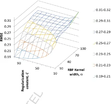
Here, the as the kernel width. Both the C and are determined by a grid search process (Goyal et al., 2014; Deo et al., 2016b; Deo et al., 2016c).
2.4 Standardized Precipitation Index
In order to develop a drought forecasting model for the study region, the monthly Standardized Precipitation Index (SPI) was first computed following McKee et al. (1993). In general, computing SPI involves fitting the gamma probability density function to the given distribution of monthly rainfall (P) data. The gamma distribution function is defined by its probability density function, g (P):
/ 1 ) ( 1 )
(P P e x
ACCEPTED MANUSCRIPT
where parameters, and , can be estimated using the maximum likelihood solution:
3
4 1 41 1 A
A (16) _ P
(18)
and A ln(P)
ln(P)
/N__
, and N = the number of rainfall observation months. The
cumulative probability can be given by
dP e x dP P g P G P P P 0 / 1
0 ( )
1 ) ( ) (
(19)
Letting t = P /, Eq. (19) becomes an incomplete gamma function:
dt e t P G t t 0 1 ) ( 1 ) (
(20)
As the gamma function is undefined for P = 0, the cumulative probability becomes:
H (P) = q + (1- q) G (P) (21)
where q is the probability of zero. The cumulative probability H (P) can be transformed into the standard normal random variable with mean zero and variance of one. This yields the monthly value of SPI, viz:
5 . 0 ) ( 0 , 1 0 . 1 ) ( 5 . 0 , 1 3 3 2 2 1 2 2 1 0 3 3 2 2 1 2 2 1 0 P H t d t d t d t c t c c t P H t d t d t d t c t c c t SPI (22)
In Eq. (22), t is given by:
0 . 1 ) ( 5 . 0 )] ( 0 . 1 [ 1 ln 5 . 0 ) ( 0 )] ( [ 1 ln 2 2 P H P H P H P H t (23)
In Eq. (23), the constants are as follows: c0 = 2.515517, c1 = 0.802853, c2 = 0.010328, d1 = 1.432788, d2 = 0.189269 and d3 = 0.001308 (McKee et al., 1993). The ‘drought’ part of the SPI range can be split into the ‘moderately dry’ (−1.5 < SPI ≤ 1.0), ‘severely dry’ (−1.5 ≤ SPI < −2.0), and ‘extremely dry’ (SPI ≤ −2.0) categories.
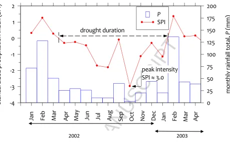
[image:11.595.66.529.83.591.2]< Fig. 2 >
ACCEPTED MANUSCRIPT
(1967, 1991), the onset of drought can be taken the month when the SPI value declines below 0 and the termination of drought when the SPI first returns to positivity. Within this drought period that is consistent with a significant reduction in the cumulative monthly rainfall, the duration of drought event can be taken as the sum of all months with SPI < 0 and the peak intensity when the SPI value is at its minimum value.
3.0 Materials and Method
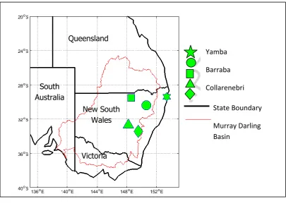
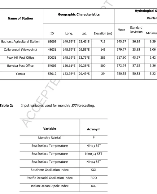
3.1 Study Area and DataIn this study a set of drought forecasting models, based on the SPI time-series, were employed for five meteorological sites (Fig. 3). The sites are located in eastern Australia (state of New South Wales) where drought is a common occurrence and leads to consequences for agricultural activities in the Murray Darling Basin (Deo et al., 2009; Helman, 2009; McAlpine et al., 2009). Table 1 lists the geographical and hydrological statistics for annual data averaged over a period from 1915–2012. The sites depict diverse climatic features with elevations from 29–713 m year-1 and mean annual rainfall from 279.77–750.35 mm year1 with a standard deviation of 23.93– 50.83 mm year-1. The climatologically averaged minimum rainfall is 1.06 mm year-1 (Collarenebri) and maximum rainfall is 9.39 mm year-1 (Bathurst Agricultural Station). Apart from Yamba Station which is located in the coastal end of eastern Australia, the other stations (Bathurst Agricultural, Collarenebri, Peak Hill, Barraba and Yamba) are situated in Murray Darling Basin. Therefore, drought modelling in this region is considered as a novel task for the management of drought-risk to the agricultural sector.
< Table 1>
< Fig. 3>
ACCEPTED MANUSCRIPT
Consequently these data have since been used for climate studies (Suppiah and Hennessy, 1998; Alexander et al., 2006; Deo and Şahin, 2015b, a; Deo et al., 2016a; Deo et al., 2016b).
As data-driven models rely on predictive features in historical data to forecast future drought, climate indices and sea surface temperature (SST) were used as regression covariates to feed in such attributes and data patterns for the respective drought model. The climate of eastern Australian responds to oceanic phases, defined by the Southern Oscillation Index (SOI), Pacific Decadal Oscillation Index (PDO), Indian Ocean Dipole (IOD) and ENSO Modoki Index (EMI) and Nino 3.0, Nino 3.4 and Nino 4.0 SST (Nicholls, 2004; Helman, 2009; Ummenhofer et al., 2009; Dijk et al., 2013). In earlier studies, the PDO and IOD phases were associated with drought (McKeon et al., 2004; McAlpine et al., 2009), and rainfall and streamflow patterns in central and southern parts of Murray Darling Basin exhibit significant perturbations due to SOI, PDO and IOD phases (Verdon and Franks, 2006; McGowan et al., 2009). When central eastern Pacific region’s SST is warm and PDO is in positivity, eastern Australia is generally warm and dry (Jones et al., 1996; Power et al., 1999; Ummenhofer et al., 2009). Similarly, EMI moderates austral autumn rainfall (Ashok et al., 2007; Cai and Cowan, 2009). Considering this, no single index can fully explain how the future drought will evolve (Helman, 2009). Therefore, the study utilised the SOI and IOD data (Australian Bureau of Meteorology) (Trenberth, 1984), PDO (Joint Institute of Study of Atmosphere and Ocean) (Mantua et al., 1997; Zhang et al., 1997), EMI (Japanese Agency for Marine Earth Science and Technology) (Ashok et al., 2007; Weng et al., 2007; Weng et al., 2009), and SST (National Prediction Centre) as the predictor variables for MARS, LSSVM and M5Tree models.
<Table 2> 3.2 Drought Model Development
To validate the potential utility of data-driven algorithms for drought modelling at five study sites in eastern Australia, the drought models were developed using MATLAB software. The predictor variables (x) comprised monthly observations of rainfall, sea surface temperature (Nino 3.0, Nino 3.4 and Nino 4.0 SST), and climate indices (SOI, PDO, IOD and EMI) for the period 1915–2012 (Table 2). The data were partitioned in the 50:25:25 ratios to create the training (01/1915–12/1963) and validation/testing sets (01/1964–12/2012), respectively (Table 3).
<Table 3>
ACCEPTED MANUSCRIPT
and predictor variable (x) (Mishra and Singh, 2010, 2011), determining the appropriate set of inputs to provide an accurate and reliable forecast model is challenging (Abbot and Marohasy, 2014). A useful preliminary step is to examine the individual relationships between x and the target output (i.e. SPI). Therefore, in this study, the cross correlation coefficient, rcross, between objective (y SPI) and predictor variable (x) in the training period was acquired to check the role of predictor in modelling the drought index. The magnitude of rcross which measures similarity between y and shifted (lagged) copies of xi = (x1, x2... xM – 1) and y = (y1, y2... yN – 1) was given by the covariance:
min( 1 , 1)) , 0 max(
, , ( 1),...,0,...,( 1)
N k M k j k j k
xy x k M N
(24.1) ) 0 ( ) 0 ( ) ( ) ( yy xx xy cross t t r (24.2)
where rcross(t) is expected to vary between -1 and 1 for any t (lagged timescale). Table 4 shows the cross correlation of inputs (versus SPI) where statistically significant correlation at the 95% level of confidence is indicated. The strongest and statistically significant correlation coefficient with 0.833rcross0.897is obtained for rainfall as a predictor variable for SPI followed by SOI (0.211rcross0.247) and Nino 4.0 SST (0.159rcross0.131). The value of rcross for the case of Nino3.4 SST as a predictor variable was also statistically significant, albeit the strength of correlation was relatively weaker. According to this result, the study utilized rainfall as a mandatory input variable for SPI forecasting.
<Table 4>
ACCEPTED MANUSCRIPT
Lin, 2003; Hsu et al., 2008), it is evident that for a given combination of C and , the RMSE value for the model obtained is unique. Thus, for all stations considered, the magnitude of LSSVM model parameters were optimised to reduce model error. The drought models were evaluated according to the agreement between forecasted and observed SPIs within the validation period.
<Fig. 3>
3.3 Model Evaluation Criteria
In the model evaluation phase, one must not rely on a single statistical metric but rather should utilise a range of performance indicators to validate the drought modelling skills from different perspectives (Krause et al., 2005; Dawson et al., 2007). In this study, the accuracy of MARS, LSSVM and M5Tree was evaluated primarily using the root mean square error (RMSE), mean absolute error (MAE) and coefficient of determination (r2) (Krause et al., 2005), viz:
N i f i o i SPI SPI N RMSE 1 2 , , 1 (25)
N i f i o i SPI SPI N MAE 1 , , 1 (26) 1 1 , 2 2 1 ____ , 2 1 ____ , ____ , 1 ____ ,2
R SPI SPI SPI SPI SPI SPI SPI SPI r N i f f i N i o o i f f i N i o o i (27)where N (=294) was the number of test samples, SPIo and SPIf were the ith value of the observed and forecasted SPIs in validation/testing period.
ACCEPTED MANUSCRIPT
In this study, drought models were developed and tested for geographically diverse sites in eastern Australia that exhibit different climatic patterns. To compare results for different sites, the normalised form of MAE, represented as the percentage inaccuracy of the forecasted relative to the observed SPI, was computed viz:
100 0 , 100 1 1 , , ,
MAPE SPI SPI SPI N MAPE Ni io
o i f
i
(28)
The Willmott’s Index (WI), which in fact resolves the potential bias issues in RMSE, was also determined (Willmott, 1981; Krause et al., 2005):
1 0 , 1 1 2 , ____ , , ____ , 1 2 , ,
d SPI SPI SPI SPI SPI SPI WI N i o i o i o i p i N i p i o i (29)It is noteworthy that the WI is advantageous over the RMSE and the R2 value where the differences in monthly SPI from observed and forecasted data are described as squared values, hence larger values of the forecasted SPI are overestimated, whereas smaller values are neglected (Legates and McCabe, 1999). However, WI was able to overcome this insensitivity of model error (Willmott, 1981), as the ratio of mean square error is considered rather than the square of the error differences (Willmott, 1984).
4.0 Results and Discussion
In this section, results attained from MARS, LSSVM and M5Tree for forecasting monthly SPI in eastern Australia are assessed to validate their adequacy in drought modelling study. The SPI forecasted using MARS was analysed where the importance of input variables was checked in terms of the predictive accuracy. Then, MARS, LSSVM and M5Tree were compared, based on statistical performance criteria (Eq. 25–29), including a seasonal analysis of model accuracy.
[image:16.595.65.529.141.368.2]ACCEPTED MANUSCRIPT
observed SPIs were examined for each site and the respective input combinations to generate a total of nine modelling scenarios (M1–M9) (see Table 5).
<Table 5>
According to the results presented in the testing period, a significant dependence of the model accuracy on the geographic distribution of stations was demonstrated where different input combinations were necessary for attaining the most accurate predictive model. Consider, for example, the case of Bathurst Agricultural Station; the MARS model utilised rainfall, all of the three SSTs data, SOI and the month to yield the lowest value of RMSE/MAE and the highest R2 value of approximately 0.159, 0.159 and 0.976, respectively, whereas for Collarenebri, the most accurate result was attained without SOI as a predictor variable (Table 5a). A closer examination of this result also showed that if redundant variables were included in the MARS model, the performance either remained stationary or declined for some study sites. This was true for the case of the Bathurst Agricultural Station, where the model M5 exhibited a value of R2 = 0.957 and RMSE/MAE = 0.222/0.174 with rainfall, SSTs and SOI as the predictor variables, but the inclusion of PDO, IOD and EMI did not improve the model’s forecasting accuracy.
<Fig. 5>
ACCEPTED MANUSCRIPT
While it is unambiguous that the optimum MARS model for Bathurst Agricultural Station, and Collarenebri and Yamba stations did not require the PDO, IOD and EMI data as input variables, the forecasted results for Peak Hill and Barraba stations were in fact significantly dependent on these data (including SOI) as a predictor variable (Table 4c-d). Despite a certain degree of variation in terms of how each of the input variables acts to moderate the r2 and RMSE/MAE values, an overall improvement in model performance was evident when all nine
predictor variables for Peak Hill and the eight predictor variables for Barraba station were incorporated in the MARS model. Clearly, this indicated that the optimum MARS model responded quite differently to the different input variables used as predictors (Table 5). Likewise, the accuracy of the MARS model exhibited a significant variability in its overall performance based on the geographic distribution of the present study sites (Fig. 2). It is noteworthy that the role of periodicity in drought forecasting was clearly demonstrated by the MARS model, where an improvement in performance was evident for the sites with month as a predictor variable.
<Fig. 6>
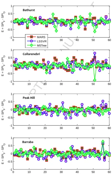
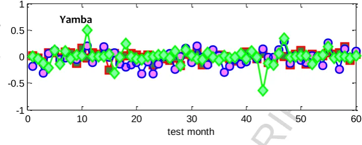
In Fig. 6 the forecasting error, E = SPIF – SPIO, deduced in the last five years of testing data for MARS, LSSVM and M5Tree models is shown, where the month (periodicity) was utlilised as a predictor variable in addition to the other variabales (Table 2). To also demonstrate the model’s statistical performance with and without periodicity, Table 6 compares the results for MARS, M5Tree and LSSVM models with only the optimum input combinations. In terms of the agreement between observed and forecasted SPIs for the best model, the time-series plot of error values depicted the MARS and M5Tree models as being more accurate than the LSSVM model, especially for Bathurst Agricultural Station, and Collarenebri and Yamba stations, where the amplitudes of E were generally smaller for majority of the test points. However, when RMSE, MABE and r2 values were compared in the testing period (Table 6), the MARS model performed better (RMSE = 0.132, r2 = 0.980) than the other two counterparts for the case of Peak Hill and Yamba stations, whereas the M5Tree model yielded better performance for the case of Collarenebri and Barraba stations (RMSE = 0.174, r2 = 0.971 and RMSE = 0.179, r2 = 0.974, respectively). For the case of Bathurst Agricultural Station, LSSVM produced modestly better forecasts (RMSE = 0.159, MAE = 0.109, r2= 0.977) than the MARS (RMSE = 0.159, MAE = 0.150, r2= 0.976) and M5Tree ((RMSE = 0.244, MAE = 0.150, r2= 0.948) models. Consistent with the MARS model (Table 5; Fig. 6), for all stations considered the LSSVM and M5Tree models also yielded significantly better results where periodicity was utilized as a predictor variable.
ACCEPTED MANUSCRIPT
As the geographic locations of study sites are diverse (Fig. 2), as also stipulated by distinct hydrological conditions (Table 1), comparison of the relative forecasting errors should be made in order to assess the model’s accuracy for one site relative to another (Krause et al., 2005; Dawson et al., 2007; Deo et al., 2016c). Thus, Willmott’s index of agreement (WI) and the mean absolute percentage error (MAPE) (%) deduced in accordance with Eq. 28 and 29 for the MARS, LSSVM and M5Tree models were made. Table 7 lists the values of WI and MAPE. For the case of Bathurst Agricultural Station, it was interesting to note that in contrast to the conclusion reached on the basis of RMSE, MAE and r2 where LSSVM was better than MARS and M5Tree models (Table 6), the model evaluation based on WI and MAPE suggested that the MARS model was more accurate (WI = 0.989, MAPE = 29.05%) than LSSVM and M5Tree (0.988, 34.164% and 0.977, 50.86%, respectively) (Table 7). However, without ignoring the fact that the differences between MARS and LSSVM was marginal (Table 6), it can be construed that both MARS and LSSVM models appear to be suitable for SPI-based forecasting Bathurst Agricultural Station.
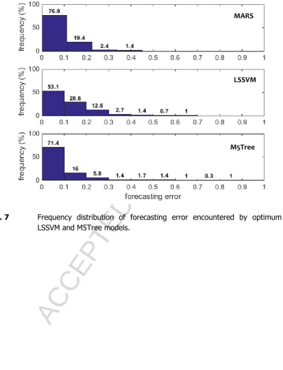
For the cases of Peak Hill and Yamba stations, the MAPE and WI clearly stipulate the superiority of MARS over LSSVM and M5Tree models. When the values of MAPE and WI were evaluated for the case of Collarenebri and Barraba stations, the results in Table 7 revealed a dramatically better performance of M5Tree with MARS and LSSVM models being significantly erroneous. That is, the magnitude of MAPE was approximately 46.77 and 39.18% (for Collarenebri) and 43.833 and 79.30% (for Barraba) relative to 29.098 and 37.94% generated by the M5Tree model. This indicated that an SPI-based drought forecasting model using M5Tree model should preferentially be adopted over the MARS and LSSVM models. However, the M5Tree model should incorporate the monthly cycle as a predictor variable so that the drought evolution over time is considered to yield more accurate and reliable forecasting performance.
<Fig. 7>
ACCEPTED MANUSCRIPT
accede the deduction made according to the mean absolute percentage error for Collarenebri and Barraba (Table 7), it contrasted the results for Peak Hill station where the MAPE value was the lowest for the MARS model. This showed that although the overall performance with the MARS model was better for Peak Hill, the MARS model could produce a majority of the forecasting errors in the test period with small error magnitudes (Fig. 7).
<Table 8>
So far, an evaluation of the prescribed data-driven models was restricted to the assessment of the forecasted and observed SPI values in the entire test dataset (1998–2012), including the cases of negative SPI (dry condition) and positive SPI (wet condition). However, in real-time drought forecasting, it is vital to clearly establish whether the prescribed MARS, LSSVM and M5Tree models are accurate enough to be able to simulate the drought segment of the SPI, as such information is more useful for drought-risk and water resources management. The exclusion of non-drought part of SPI for drought model assessment is also important as it provides the modeler crucial information on whether the model is able to represent future drought cases adequately. Table 8 shows a closer analysis of forecasting results of the drought part of SPI within the test period, where the relative forecasting error (%) in respect of the observed SPI ≤ -2.0 (extreme drought), -1.5 ≤ SPI < -2.0 (severe drought) and -0.5 ≤ SPI < 1.5 (moderate drought) is summarized.
ACCEPTED MANUSCRIPT
While M5Tree was found to be relatively superior to the MARS and LSSVM models for a majority of the sites, there appeared to be a significant dependence of the respective model performance on the geographic distribution of sites. For example, in the case of extreme drought forecasts, M5Tree was more accurate than MARS for all sites except Peak Hill. In fact, for the latter station, MARS outperformed the M5Tree model, where relative forecasting errors of 0.20% compared with 4.9% (M5Tree) and 37.2% (LSSVM) were recorded (Table 8a). The model developed for severe and moderate drought forecasting found M5Tree as being more accurate than MARS when tested for Collarenebri, Barraba and Yamba stations (MAPE 3.0– 5.2%) compared to 6.6% and 1.3% for Bathurst and Yamba stations (Table 8b). Accordingly, it can be concluded that the drought models exhibited a strong geographic behavior in their accuracy, which shows the complexity of drought behavior and the different data attributes and patterns in the predictor variables used to forecast SPI. Notwithstanding this, it is perceived that while MARS exhibited an overall better performance for a number of stations when evaluated for the entire test data (Tables 6 and 7), the M5Tree model resulted in much better accuracy when the drought segment of the test signal was analyzed (Table 8).
ACCEPTED MANUSCRIPT
Table 9>
5.0 Further Discussion, Limitations and Future Work
The results acquired for modelling monthly SPI using the MARS, LSSVM and M5Tree algorithms highlighted a pivotal role of periodicity as a crucial driver of model accuracy, among other predictors in order of their relative importance. This was clearly evident by the improved performance of models with monthly cycle as an input, which yielded lower RMSE, MAE and larger r2 (Tables 5 and 6) compared to the forecasts without applying the periodicity factor. These results also resonate with those of other investigations (e.g. (Kane and Trivedi, 1986; Kane, 1997; Almedeij, 2015; Moreira et al., 2015)), where periodicity in the drought behavior was found to be associated with the seasonality of input variables and the respective phases of atmospheric-oceanic oscillation, such as the quasi-biennial oscillation (QBO), solar activity, ENSO, Inter-decadal Pacific Oscillation (IPO) and intensification of subtropical ridge (Verdon and Franks, 2006; Verdon‐Kidd and Kiem, 2009; Timbal et al., 2010; Gallant et al., 2013; Almedeij, 2015). Although climate indices, including SOI, PDO, IOD, EMI and SSTs, were utilized in different combinations to model the SPI time-series, the greater importance of SST and the respective month in the model’s training period as a predictor was evident. Lyon et al. (2012) showed a significant improvement in SPI prediction using seasonality in precipitation as an important characteristic of the local climate. In general, seasonality in the precipitation variance was seen to appreciably enhance the predictive skills derived from the drought indicator with substantial variation, depending on the location and season considered. In our study, the use of seasonality was very important for accurately modelling SPI at all study sites, leading to a marked improvement in model performance (Tables 5, 6 and 7). Therefore, our results reinforce the importance of periodicity as an important determinant of drought modelling accuracy.
ACCEPTED MANUSCRIPT
of models at these stations compared to Bathurst, Collarenebri and Barraba. Although the exact cause of this is not known, it is possible that the changes in rainfall and other drought indicators (e.g. SOI) were more closely linked to the cyclic behavior of ocean and atmospheric phases. Earlier studies that developed data-driven models based on a combination of climate indices, SSTs and rainfall found similar variability of the model accuracy over large, sparsely distributed areas (Abbot and Marohasy, 2012, 2014; Deo and Şahin, 2015b, a; Deo et al., 2016b). Therefore, the importance of identifying the most appropriate predictor variable for monthly SPI forecasting remains a paramount task for accurate modelling of drought behavior.
The distinct geographic behaviour of the drought model accuracy was clearly consistent with an earlier study that developed an ANN model for the prediction of the Standardized Precipitation and Evapotranspiration Index (Deo and Şahin, 2015a) and the Effective Drought Index (Deo and Şahin, 2015b). The former study, which also employed rainfall, climate indices and SST data, reported better estimation accuracy for Yamba than for Bathurst Agricultural Station. Therefore, it is perceived that the accuracy of drought models at different study sites is expected to vary in view of the high variability established in the relationships between climate indices, SSTs and rainfall data over different spatial and temporal domains (Nicholls, 2004; Schepen et al., 2012). The evaluation of models over monthly and seasonal scales showed that LSSVM was generally inferior to MARS and M5Tree (Table 9). While the exact cause of this is not known as the models adopt a black-box approach for extracting predictive features in the training dataset, other studies in evaporation modelling (Kisi, 2015, 2016) also found similar results. Importantly, when drought cases (for months with SPI < 0) were analysed in the test period, the M5Tree model showed dramatically better performance for a majority of the stations in moderate, severe and extreme drought categories.
ACCEPTED MANUSCRIPT
developing the drought model. Owing to the elusive definition of drought and its insidious and complex nature where the effect of a predictor is not known a priori, the information deduced from serial correlation of the inputs could incorporate the inherent persistence characteristics, and therefore, help extract predictive information to improve the future drought warning (Lyon et al., 2012). In fact, the cumulative, time-integrated nature of drought events (resulting in persistence from one month to the next) was shown to be an important time-lagged driver with characteristics valuable for drought monitoring and warning (Redmond, 2002; Nicholls, 2005; Sen and Boken, 2005).
In this study, we did not adopt a pre-processing technique for input data for developing the respective drought models. One criticism of data-driven models without a pre-processing technique is their inability to account for the physics of the hydrological processes (Aksoy et al., 2007) that are necessary for accurate prediction of drought behavior. As the predictors of drought also exhibit nonlinear and non-stationary phenomenon, the presence of non-stationarity features (e.g. trends, seasonal variations, periodicity and jumps in input data) can influence the model accuracy (Tiwari and Chatterjee, 2010; Tiwari and Adamowski, 2013). Also, the relationships between inputs (e.g. rainfall, SOI) and the objective variable is generally non-linear (Montanari et al., 1996), so the non-stationarities caused by trends and seasonal variation can produce a negative impact on model performance (Adamowski et al., 2012; Deo et al., 2016b; Deo et al., 2016c). However, if a pre-processing technique (e.g. wavelet transformation) is adopted, it can extract the time-frequency information and capture the data attributes and patterns to reflect the stochasticity of input variables (Daubechies, 1990). Wavelet transformation is used as an ancillary tool for analyzing stochastic variations, periodicity and trends (Kim and Valdés, 2003; Wang and Ding, 2003; Adamowski and Sun, 2010; Kisi, 2010; Kisi and Cimen, 2011; Nalley et al., 2012; Deo et al., 2016b; Deo et al., 2016c) but is yet to be tested for drought forecasting using MARS, LSSVM and M5Tree. In a follow-up study, wavelet transformation or an alternative data pre-processing tool can be applied to enhance the performance of the prescribed drought models. Additionally, the importance of, and the relationship between, oceanic-atmospheric drivers (e.g. SST) and the respective drought index (e.g. SPI) could potentially be identified by incorporating nonlinear input variable selection (May et al., 2008; Salcedo-Sanz et al., 2014; Seo et al., 2014; Quilty et al., 2016), providing an alternative pathway for deducing the most relevant input variables for improved performance of SPI models.
ACCEPTED MANUSCRIPT
ACCEPTED MANUSCRIPT
advocated that the selection of drought models based on a given data-driven techniques is not achievable without challenges, thus, drought modelling may be tackled appropriately by enhancing the understanding and complexity of model inputs (predictor variables) in relation to the drought behavior and how these patterns and attributes are extracted to develop the actual drought forecasts. Finally, a drought model accuracy is expected to be only dependent on the considered model’s mathematical and computational frameworks but also on the interactions of the predictive features within the input variables utilized and the non-linear associations with the respective response variable (drought index).
Acknowledgment
The precipitation data were from Australian Bureau of Meteorology and climate indices and SST from the Joint Institute of Study of Atmosphere and Ocean and Japanese Agency for Marine-Earth Science and Technology. USQ Academic Division funded first author (Dr RC Deo) through “Research Activation Incentive Scheme (RAIS, July–September 2015)” to collaborate with Professor Ozgur Kisi (Canik Basari University, Turkey) and Distinguished Professor Vijay P. Singh, Texas A&M University (USA). Dr RC Deo held Endeavour Executive Fellowship (4293–2015) funded by the Australian Government. We also thank the reviewer and Editor-in-Chief for their insightful comments on this paper.
Figure Captions
Fig. 1. Structures of MARS, M5Tree and LSSVM models.
Fig. 2 Monthly standarized precipitation index with drought characteristics and rainfall data for millennium drought (January 2002–April 2003) for Bathurst Agricultural Station.
Fig. 3 Location of study sites in eastern New South Wales (NSW).
ACCEPTED MANUSCRIPT
Fig. 5 Scatterplot of forecasted (SPIF) and observed (SPIO) standardized precipitation index (SPI) using the MARS model with and without periodicity (i.e. month) as an input parameter with a linear regression equation.
Fig. 6 Forecasting error, E = SPIF – SPIO for MARS, LSSVM and M5Tree (with periodicity as an input variable) in the last 5 years of testing period.
Fig. 7 Frequency distribution of forecasting error encountered by optimum MARS, LSSVM and M5Tree models.
Table Captions
Table 1: Descriptive statistics of the study sites.
Table 2: Input variables used for monthly SPI forecasting.
Table 3: The partitioning of input data into training, validation and testing sets.
Table 4: Cross correlation of inputs (with SPI). rcross in boldface are statistically significant with 95% confidence.
Table 5: Influence of input combinations for forecasting of SPI using a MARS model measured by root mean square error (RMSE), mean absolute error (MAE) and coefficient of determination (R2). Note: optimum model for each site is
boldfaced (blue).
Table 6: Comparison ofMARS, M5 Tree and LSSVM models with optimum inputs with and without periodicity.
Table 7: Comparison of optimum MARS, LSSVM and M5Tree according to Willmott’s index (WI) and mean absolute percentage error (MAPE, %) with and without periodicity.
Table 8: Forecasting skill of optimum MARS, M5Tree and LSSVM in terms of mean absolute percentage error, MAPE (%) for different categories of drought events within the test period.
Table 9: Analysis of mean absolute percentage error, MAPE (%), over seasonal scales.
ACCEPTED MANUSCRIPT
Table A2 The regression tree for the optimal M5Tree models in modeling SPI-Bathurst.
References
Abbot, J., Marohasy, J.2012.Application of artificial neural networks to rainfall forecasting in Queensland, Australia Adv. Atmos. Sci.29, pp. 717-730.
Abbot, J., Marohasy, J.2014.Input selection and optimisation for monthly rainfall forecasting in Queensland, Australia, using artificial neural networks Atmos. Res.138, pp. 166-178.
Abraham, A., Steinberg, D. 2001 Is neural network a reliable forecaster on earth? a MARS query! , Bio-Inspired Applications of Connectionism, Springer, pp. 679-686.
Adamowski, J., Fung Chan, H., Prasher, S.O., Ozga‐Zielinski, B., Sliusarieva, A.2012.Comparison of multiple linear and nonlinear regression, autoregressive integrated moving average, artificial neural network, and wavelet artificial neural network methods for urban water demand forecasting in Montreal, Canada Water Resour. Res.48.
Adamowski, J., Karapataki, C.2010.Comparison of multivariate regression and artificial neural networks for peak urban water-demand forecasting: evaluation of different ANN learning algorithms
Journal of Hydrologic Engineering15, pp. 729-743.
Adamowski, J., Sun, K.2010.Development of a coupled wavelet transform and neural network method for flow forecasting of non-perennial rivers in semi-arid watersheds J. Hydrol.390, pp. 85-91.
Aksoy, H., Guven, A., Aytek, A., Yuce, M.I., Unal, N.E.2007.Discussion of “Generalized regression neural
networks for evapotranspiration modelling” Hydrological Sciences Journal52, pp. 825-831.
Alexander, L. et al.2006.Global observed changes in daily climate extremes of temperature and precipitation Journal of Geophysical Research: Atmospheres (1984–2012)111.
Alexandersson, H.1986.A homogeneity test applied to precipitation data Journal of climatology 6, pp. 661-675.
Almedeij, J.2015.Long-term periodic drought modeling Stochastic Environmental Research and Risk Assessment, pp. 1-10.
Ashok, K., Behera, S.K., Rao, S.A., Weng, H., Yamagata, T.2007.El Niño Modoki and its possible teleconnection Journal of Geophysical Research: Oceans (1978–2012)112.
Bates, B., Kundzewicz, Z.W., Wu, S., Palutikof, J. 2008 Climate change and water: Technical paper vi. Intergovernmental Panel on Climate Change (IPCC).
Belayneh, A., Adamowski, J.2012.Standard precipitation index drought forecasting using neural networks, wavelet neural networks, and support vector regression Applied Computational Intelligence and Soft Computing2012, p. 6.
Bhattacharya, B., Solomatine, D.P.2005.Neural networks and M5 model trees in modelling water level–
discharge relationship Neurocomputing63, pp. 381-396.
Bishop, C.M. 1995 Neural networks for pattern recognition. Oxford university press.
BOM High-quality Australian Daily Rainfall Dataset. National Climate Centre, Bureau of Meteorology, Melbourne, Victoria (2008).
Brown, S.C., Versace, V.L., Lester, R.E., Walter, M.T.2015.Assessing the impact of drought and forestry on streamflows in south-eastern Australia using a physically based hydrological model
Environmental Earth Sciences74, pp. 6047-6063.
Butte, N.F. et al.2010.Validation of cross-sectional time series and multivariate adaptive regression splines models for the prediction of energy expenditure in children and adolescents using doubly labeled water The Journal of nutrition140, pp. 1516-1523.
Cai, W., Cowan, T.2008.Evidence of impacts from rising temperature on inflows to the Murray‐Darling Basin Geophysical research letters35.
ACCEPTED MANUSCRIPT
Cancelliere, A., Bonaccorso, B., Mauro, G.2006.A non-parametric approach for drought forecasting through the standardized precipitation index Metodi statisticie matematici per l Analisi delle serie idrologiche1, pp. 1-8.
Cancelliere, A., Di Mauro, G., Bonaccorso, B., Rossi, G.2007.Drought forecasting using the standardized precipitation index Water. Resour. Manag.21, pp. 801-819.
Cheng, M.-Y., Cao, M.-T.2014.Accurately predicting building energy performance using evolutionary multivariate adaptive regression splines Applied Soft Computing22, pp. 178-188.
Cherkassky, V., Mulier, F.M. 2007 Learning from data: concepts, theory, and methods. John Wiley & Sons.
Choubin, B., Malekian, A., Gloshan, M.2016.Application of several data-driven techniques to predict a standardized precipitation index Atmósfera29, pp. 121-128.
Craven, P., Wahba, G.1978.Smoothing noisy data with spline functions Numerische Mathematik31, pp. 377-403.
Crimp, S. et al.2015.Bayesian space–time model to analyse frost risk for agriculture in Southeast Australia Int. J. Climatol.35, pp. 2092-2108.
Daubechies, I.1990.The wavelet transform, time-frequency localization and signal analysis Information Theory, IEEE Transactions on36, pp. 961-1005.
Dawson, C.W., Abrahart, R.J., See, L.M.2007.HydroTest: a web-based toolbox of evaluation metrics for the standardised assessment of hydrological forecasts Environmental Modelling & Software22, pp. 1034-1052.
Deo, R.C., Byun, H.-R., Adamowski, J.F., Begum, K.2016a.Application of effective drought index for quantification of meteorological drought events: a case study in Australia Theoretical and Applied Climatology, pp. 1-21.
Deo, R.C., Şahin, M.2015a.Application of the Artificial Neural Network model for prediction of monthly
Standardized Precipitation and Evapotranspiration Index using hydrometeorological parameters and climate indices in eastern Australia Atmos. Res.161-162, pp. 65-81.
Deo, R.C., Şahin, M.2015b.Application of the extreme learning machine algorithm for the prediction of
monthly Effective Drought Index in eastern Australia Atmos. Res.153, pp. 512-525.
Deo, R.C., Şahin, M.2016.An extreme learning machine model for the simulation of monthly mean
streamflow water level in eastern Queensland Environmental Monitoring and Assessment DOI (10.1007/s10661-016-5094-9).
Deo, R.C., Samui, P., Kim, D.2015.Estimation of monthly evaporative loss using relevance vector machine, extreme learning machine and multivariate adaptive regression spline models
Stochastic Environmental Research and Risk Assessment, pp. 1-16.
Deo, R.C. et al.2009.Impact of historical land cover change on daily indices of climate extremes including droughts in eastern Australia Geophysical Research Letters36.
Deo, R.C., Tiwari, M.K., Adamowski, J., Quilty, J.2016b.Forecasting Effective Drought Index Using a Wavelet Extreme Learning Machine (W-ELM) Model Stochastic Environmental Research and Risk
Assessmentin press, pp. DOI: 10.1007/s00477-00016-01265-z.
Deo, R.C., Wen, X., Feng, Q.2016c.A wavelet-coupled support vector machine model for forecasting global incident solar radiation using limited meteorological dataset Applied Energy168, pp. 568–
593.
Dijk, A.I. et al.2013.The Millennium Drought in southeast Australia (2001–2009): Natural and human causes and implications for water resources, ecosystems, economy, and society Water Resour. Res.49, pp. 1040-1057.
Friedman, J.H.1991.Multivariate adaptive regression splines The annals of statistics, pp. 1-67.
Gallant, A.J., Reeder, M.J., Risbey, J.S., Hennessy, K.J.2013.The characteristics of seasonal‐scale droughts in Australia, 1911–2009 Int. J. Climatol.33, pp. 1658-1672.
Goyal, M.K., Bharti, B., Quilty, J., Adamowski, J., Pandey, A.2014.Modeling of daily pan evaporation in sub tropical climates using ANN, LS-SVR, Fuzzy Logic, and ANFIS Expert Systems with Applications
41, pp. 5267-5276.
ACCEPTED MANUSCRIPT
Hayes, M.J., Svoboda, M., Wall, N., Widhalm, M.2011.The Lincoln declaration on drought indices: universal meteorological drought index recommended Bulletin of the American Meteorological Society92, pp. 485-488.
Hayes, M.J., Svoboda, M.D., Wilhite, D.A., Vanyarkho, O.V.1999.Monitoring the 1996 drought using the standardized precipitation index Bulletin of the American Meteorological Society 80, pp. 429-438.
Haylock, M., Nicholls, N.2000.Trends in extreme rainfall indices for an updated high quality data set for Australia, 1910-1998 Int. J. Climatol.20, pp. 1533-1541.
Helman, P. Droughts in the Murrary-Darling Basin since European settlement. Griffith Centre for Coastal Management Research Report No 100, Licensed from the Murray-Darling Basin Authority under a Creative Commons Attribution 3.0 Australia Licence (2009).
Hsu, C.-W., Chang, C.-C., Lin, C.-J. A practical guide to support vector classification. (2003).
Hsu, H.-H., Hung, C.-H., Lo, A.-K., Wu, C.-C., Hung, C.-W.2008.Influence of tropical cyclones on the estimation of climate variability in the tropical western North Pacific J. Climatol.21, pp. 2960-2975.
IPCC 2007 Summary for Policymakers. In: Climate Change 2007: The Physical Science Basis. Contribution of Working Group I to the Fourth Assessment Report of the Intergovernmental Panel on Climate
Change Cambridge University Press, United Kingdom and New York, NY, USA 1-18 pp.
IPCC 2012 Summary for Policymakers: A Special Report of Working Groups I and II of the Intergovernmental Panel on Climate Change. in: Field, C.B. et al. (Eds.), In: Managing the Risks of
Extreme Events and Disasters to Advance Climate Change Adaptation Cambridge University
Press, Cambridge, UK.
Jalalkamali, A., Moradi, M., Moradi, N.2015.Application of several artificial intelligence models and ARIMAX model for forecasting drought using the Standardized Precipitation Index International
Journal of Environmental Science and Technology12, pp. 1201-1210.
Joaquín Andreu et al. 2015 Drought Indicators: Monitoring, Forecasting and Early Warning at the Case Study Scale. DROUGHT-R&SPI (Fostering European Drought Research and Science-Policy Interfacing) , Collaborative Project funded by the European Commission under the FP7 Cooperation Work Programme: Theme 6: Environment (Grant agreement no: 282769).
Jones, P. et al.1996.Summer moisture availability over Europe in the Hadley Centre general circulation model based on the Palmer Drought Severity Index Int. J. Climatol.16, pp. 155-172.
Kane, R.1997.Prediction of Droughts in North‐East Brazil: Role of ENSO and Use of Periodicities Int. J. Climatol.17, pp. 655-665.
Kane, R.P., Trivedi, N.B.1986.Are droughts predictable? Climatic Change8, pp. 209-223.
Keyantash, J., Dracup, J.A.2002.The quantification of drought: an evaluation of drought indices Bulletin
of the American Meteorological Society83, pp. 1167-1180.
Kim, T.-W., Valdés, J.B.2003.Nonlinear model for drought forecasting based on a conjunction of wavelet transforms and neural networks Journal of Hydrologic Engineering8, pp. 319-328.
Kisi, O.2010.Wavelet regression model for short-term streamflow forecasting J. Hydrol.389, pp. 344-353.
Kisi, O.2015.Pan evaporation modeling using least square support vector machine, multivariate adaptive regression splines and M5 model tree J. Hydrol.528, pp. 312-320.
Kisi, O.2016.Modeling reference evapotranspiration using three different heuristic regression approaches Agricultural Water Management169, pp. 162-172.
Kisi, O., Cimen, M.2011.A wavelet-support vector machine conjunction model for monthly streamflow forecasting J. Hydrol.399, pp. 132-140.
Koehn, J.2015.Managing people, water, food and fish in the Murray–Darling Basin, south‐eastern Australia Fisheries Management and Ecology22, pp. 25-32.
Krause, P., Boyle, D., Bäse, F.2005.Comparison of different efficiency criteria for hydrological model assessment Advances in Geosciences5, pp. 89-97.
Lavery, B., Joung, G., Nicholls, N.1997.An extended high-quality historical rainfall dataset for Australia
ACCEPTED MANUSCRIPT
Legates, D.R., McCabe, G.J.1999.Evaluating the use of “goodness‐of‐fit” measures in hydrologic and hydroclimatic model validation Water Resour. Res.35, pp. 233-241.
Lin, H.-T., Lin, C.-J.2003.A study on sigmoid kernels for SVM and the training of non-PSD kernels by SMO-type methods submitted to Neural Computation, pp. 1-32.
Lyon, B. et al.2012.Baseline probabilities for the seasonal prediction of meteorological drought Journal
of Applied Meteorology and Climatology51, pp. 1222-1237.
Mantua, N.J., Hare, S.R., Zhang, Y., Wallace, J.M., Francis, R.C.1997.A Pacific interdecadal climate oscillation with impacts on salmon production Bulletin of the american Meteorological Society
78, pp. 1069-1079.
Marj, A.F., Meijerink, A.M.2011.Agricultural drought forecasting using satellite images, climate indices and artificial neural network International journal of remote sensing32, pp. 9707-9719.
May, R.J., Maier, H.R., Dandy, G.C., Fernando, T.G.2008.Non-linear variable selection for artificial neural networks using partial mutual information Environmental Modelling & Software 23, pp. 1312-1326.
McAlpine, C. et al.2007.Modeling the impact of historical land cover change on Australia's regional climate Geophysical Research Letters34.
McAlpine, C. et al.2009.A continent under stress: interactions, feedbacks and risks associated with impact of modified land cover on Australia's climate Global Change Biology15, pp. 2206-2223. McGowan, H.A., Marx, S.K., Denholm, J., Soderholm, J., Kamber, B.S.2009.Reconstructing annual inflows
to the headwater catchments of the Murray River, Australia, using the Pacific Decadal Oscillation Geophysical Research Letters36.
McKee, T.B., Doesken, N.J., Kleist, J. The relationship of drought frequency and duration to time scales.
Proceedings of the 8th Conference on Applied Climatology, American Meteorological Society Boston, MA (1993), pp. 179-183.
McKeon, G., Hall, W., Henry, B., Stone, G., Watson, I.2004.Pasture degradation and recovery in Australia's rangelands: learning from history.
Mishra, A.K., Desai, V.2005.Drought forecasting using stochastic models Stochastic Environmental
Research and Risk Assessment19, pp. 326-339.
Mishra, A.K., Singh, V.P.2010.A review of drought concepts J. Hydrol.391, pp. 202-216. Mishra, A.K., Singh, V.P.2011.Drought modeling–A review J. Hydrol.403, pp. 157-175.
Mitchell, T.M.1997.Machine learning Computer Science Series (McGraw-Hill, Burr Ridge, 1997) MATH. Montanari, A., Rosso, R., Taqqu, M.S.1996.Some long‐run properties of rainfall records in Italy Journal
of Geophysical Research: Atmospheres (1984–2012)101, pp. 29431-29438.
Moreira, E., Martins, D., Pereira, L.2015.Assessing drought cycles in SPI time series using a Fourier analysis Natural Hazards and Earth System Sciences15, pp. 571-585.
Mpelasoka, F., Hennessy, K., Jones, R., Bates, B.2008.Comparison of suitable drought indices for climate change impacts assessment over Australia towards resource management Int. J. Climatol. 28, pp. 1283-1292.
Müller, K.-R. et al. 1997 Predicting time series with support vector machines. Artificial Neural
Networks—ICANN'97, Springer Berlin Heidelberg, Switzerland, pp. 999-1004.
Nalley, D., Adamowski, J., Khalil, B.2012.Using discrete wavelet transforms to analyze trends in streamflow and precipitation in Quebec and Ontario (1954–2008) J. Hydrol.475, pp. 204-228. Nicholls, N.2004.The changing nature of Australian droughts Climatic change63, pp. 323-336.
Nicholls, N., M. J. Coughlan, and K. Monnik, 2005 2005 The Challenge of Climate Prediction in Mitigating Drought Impacts. in: Wilhite, D.A. (Ed.), Drought and Water Crises: Drought andWater Crises, Science Technology and Management Issues,, Taylor and Francis: , 33–51., p. 33.
Okkan, U., Serbes, Z.A.2012.Rainfall–runoff modeling using least squares support vector machines
Environmetrics23, pp. 549-564.
Power, S. et al.1999.Decadal climate variability in Australia during the twentieth century Int. J. Climatol.
ACCEPTED MANUSCRIPT
Quilty, J., Adamowski, J., Khalil, B., Rathinasamy, M.2016.Bootstrap rank‐ordered conditional mutual information (broCMI)—A nonlinear input variable selection method for water resources modeling Water Resour. Res.
Quinlan, J.R. Learning with continuous classes. 5th Australian joint conference on artificial intelligence, Singapore (1992), pp. 343-348.
Qureshi, M., Ahmad, M., Whitten, S., Reeson, A., Kirby, M.2016.Impact of Climate Variability Including Drought on the Residual Value of Irrigation Water Across the Murray–Darling Basin, Australia
Water Economics and Policy, p. 1550020.
Rahimikhoob, A., Asadi, M., Mashal, M.2013.A comparison between conventional an