Confidence intervals for reliability growth models with small sample sizes

Confidence Intervals for Reliability Growth Models with Small Sample Sizes

John Quigley, Lesley Walls

University of Strathclyde, Glasgow, Scotland

Key Words

Reliability growth models, Order statistics, Confidence intervals

Reader Aids

Purpose: Widen the state of the art.

Special math needed for explanations: Probability and statistics. Special math needed to use results: Probability and statistics. Results useful to: Reliability analysts, Statisticians.

Summary and Conclusions

This paper develops inference properties for a reliability growth model. The approach considered assumes a prior distribution for the ultimate number of faults that would be exposed if testing were to continue ad infinitum but estimates the parameters of the intensity function empirically. A fixed-point iteration procedure to obtain the Maximum Likelihood Estimate is investigated for bias and conditions of existence.

The main purpose for this model is to support inference in situations where failure data are few. A procedure for providing statistical confidence intervals is investigated and shown to be suitable for small sample sizes. An application of these techniques is illustrated through an example.

1. INTRODUCTION

Order statistic models assume there is a finite, but unknown, number of faults in a system and that these faults will be realized as failures through growth test. In addition, the failure times will represent realizations from an underlying probability distribution. Models developed from order statistic (OS) approaches have dominated software reliability growth modeling [1-10]. This is because such models captured the belief that once a fault had been removed from software, it is removed forever and no other faults are introduced.

failure rate. Therefore even if all significant design weaknesses are exposed during growth test, there will still exist a failure rate due to the physical nature of the system.

There are three major differences between the two approaches:

(i) the number of faults remaining undetected by an arbitrary time t is assumed an unknown constant in OS models, but a random variable in NHPP;

(ii) if testing continues infinitely then there would be a finite number of faults detected for an OS model, however for a NHPP model it would depend upon whether or not the integral over the range (0, ∞) of the intensity function diverged or converged;

(iii) the intensity function for OS models is conditional on the history of the events that have occurred by time of analysis, while a NHPP is independent of the history of the process.

failure on growth test. In this case a prior distribution may be elicited and used with an OS models structure as advocated by [18].

However OS reliability growth models are often criticized [6, 19] for supporting poor inference about the ultimate number of faults exposed through test. Therefore in this paper we derive point and interval estimators for the expected number of faults remaining in the system and the mean time to failure assuming exponential times to failure and a Poisson prior distribution. The sampling distribution of the estimator of the mean time to fault detection is obtained and the properties of the estimator are investigated for typical values of sample size parameters experienced in practice. Finally, an example of the application of the proposed model and the usefulness of the resulting estimates are illustrated for a growth test of an electronic system.

Acronyms and Notation

CDF cumulative distribution function

i.i.d. independently and identically distributed MLE maximum likelihood estimator

NHPP Non Homogeneous Poisson Process OS order stat istic

PDF probability density function

j

α expected number of faults that will be realised as ratio of observed number of faults

b observed number of faults

Fb(t) CDF of time to detection of bth fault given N ≥ b

1

γp− ratio of MLE to true hazard rate after p-1 iterations

~

 

 

 

L M t likelihood function for order statistic model

λ mean number of faults

j observed number of failures by time t′ M parameter set of order statistic model

µ hazard rate of distribution of times to realisation of faults

N number of faults

(

)

π N=n prior distribution of number of faults

j

R mean total time on test to realisation of jth fault conditioned on faults realised to date

ti accumulated test time to realisation of ith fault

'

t observed accumulated test time at point of analysis ~

t set of accumulated test times

i

W weighted sum of independently and identically distributed exponential random variables

2. ORDER STATISTIC RELIABILITY GROWTH MODEL

representation of the uncertainty about the number of potential faults (N) that will require corrective action.

In general an OS model does not require the prior probability distribution to conform to any parametric form. Although here we consider the case of a prior Poisson distribution, namely:

(

)

!

λ λ

π N =n = n e− λ> n=

n (1)

The times of fault detection are assumed i.i.d. with distribution function F(t). The number of faults ultimately detected through testing (N) is assumed greater than or equal to the observed number of faults detected (b). This results in the following PDF for the time to detection of the bth fault, tb:

(

)

[

]

[

]

1

( ) ( ) 1 ( ) , 0, 1,2,..,

1

-− −

−

 

=_{ } − > > =

 

b N b

b b b b b b b

N

f t N F t f t F t t t b N

b N b

(2) It is assumed no immediate faults are detected at time 0 and that failures are properly classified as belonging to the fault detection process. This function can be shown to integrate to 1, with a change of variable.

(

) (

)

(

) (

)

( )

( )

( )

( )

( )

(

)

1 ! ! !

1

!

1 ! 1

! λ λ λ λ π λ λ λ λ ∀ ≥ − − − ∀ ≥ − − = − ₋ − − = = = = ≥ −         − − = −     =   − _ − _  

∑

∑

∑

∑

b b b b

n b

n

b n b

b b b

n b

i b

i

b b F t

b b

i b

i

f t f t N n N n N b

n e

F t f t F t

b n b n

e i

F t f t e

e b

i

(3)

Bayesian methods can be applied to update the prior distribution using observed data at test time t′, by which time it is assumed that j failures have occurred. Following [21] the likelihood function for a OS model conditioned on a set of parameters M, where the first j faults have been detected at accumulated test time ti (i = 1 to j) and N-j faults will be

detected after accumulated test time t′ is given by:

( )

(

)

(

)

_Μ _{= −}

        

∏

L t f t M F t M

v

where:

~

1,... , '

 

= _ j _

t t t t

Thus using the relationship derived from Bayes theorem, the updated expert distribution is given by:

(

)

(

)

, 1,2,. ! λ λ π − − −     = + ≥ = =

v F t

F t e

N j v N j j

where: 0 < tj < t′ < tj+1.

This is a Poisson distribution with expectation:

~

[1 ( ')]λ

  = −    

E v t F t (5)

3. POINT ESTIMATORS FOR THE MEAN TIME TO FAULT DETECTION Assume the times to failure are exponentially and identically distributed with common hazard rate µ with PDF and CDF:

( )

(

)

( )

(

)

exp , , 0

1 exp ,

µ µ µ µ

µ µ

= − >

= − −

f t t t

F t t (6)

This OS reliability growth model was first explored by [1] using classical inference techniques and the poor performance of estimators of the parameter N are well documented. For example, [19] demonstrated that the MLE of N is unstable and inconsistent for small samples. However, following [7 and 18], who assume prior information about the number of faults present in a system, the MLE of the mean time to fault detection, i.e. µ-1 (or the mode of the updated prior distribution) can be shown to be the

random variable ^ 1

^

1 ^

' exp '

1 λ µ

µ

=

 

+ _− _

 

=

∑

j

i i

t t t

j (7)

NB: MLE’s are invariant under monotonic transformation. Therefore, the MLE of the hazard rate µ is the inverse of the MLE of the mean µ-1.

Taking the limit of equation (7) as the time approaches ∞, we obtain:

^

1 1

'

' exp '

lim

λ µ

= =

→∞

 

+ _− _

 _{ =}

∑

∑

i i

t

t t t t

j j (8)

which is the MLE of µ-1 with j i.i.d. exponential random variables. Therefore, the distribution of the estimate of the (hazard rate) mean tends to that of a(n) (Inverse) Gamma.

Thus the model appears to behave intuitively regarding both the limiting values of number of observations (i.e. j) and time of analysis (i.e. t′) by producing sensible estimates as the MLE of µ represents the observed number of failures divided by total expected exposure, which is a natural estimator of µ [23].

solution are with respect to bias and variability. We first consider the existence of the estimator then we investigate it for bias and variability.

3.1 Existence of Estimator

Consider the estimator for the mean µ-1 obtained after the pth iteration of a fixed-point iteration [24]: ( ) ( ) ( ) 1 ^ 1 1 µ λ µ − − = + =

∑

t t e

j (9)

This function can be shown to have at least one solution [25] and have three solutions (implying a bi-modal Likelihood function) if both of the following conditions are met simultaneously: ( ) 1 ( ) 0.25 = = ≤

∑

and (10)

1 1 4 ₂ 1 1 4 ₂

exp exp

2 1 1 4 α 2 1 1 4

 − −     + −   

 −   > > −   

   _{− −}     _{+ −} 

       

j j

j j j

j j

R R

R R

R R

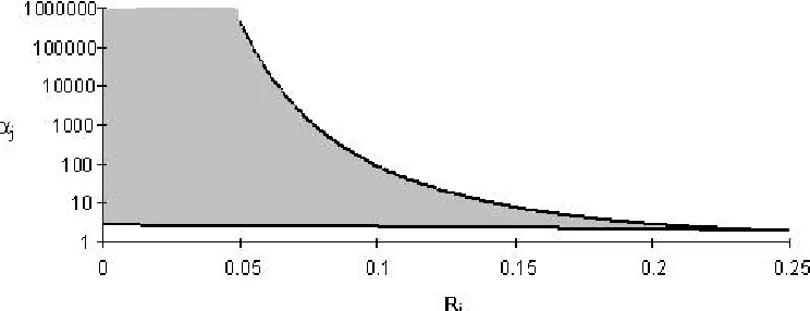
FIGURE 1

The situation where the likelihood function is bimodal is unlikely to occur for processes where faults are few, if the expert is calibrated and the model assumptions are correct. Figure 1 illustrates the region where these conditions are met. This phenomenon is discussed in greater detail in [25].

3.2 Bias of Estimator

We consider the MLE expressed as an iterative function (9) and evaluate the expectation of the estimator obtained after the pth iteration conditioned on the estimator obtained after the p-1th iteration. Furthermore, we consider the expectation in two stages, firstly conditioned on the number of faults that exist within the system, i.e. N, and then with respect to N. This allows us to consider the sum of the first j order statistics as a weighted sum of independent and identically distributed exponential random variables with mean µ-1, i.e. Wi, [21].

(

)

1 - 1

^

1 1

- 1

- 1 - 1

1 µ λ µ − = − + = = ≥ ≥  _{+   ∑}   _{+  }    _{ +  +  }   = _{ }   _{ }   _{ }  

∑

∑

N N j N N j

p

j i W W

e

N i N i

E E E E

j (11)

^

1 1 -1 1 -1

- 1 - 1 1

- 1 - 1 - 1

1 1 λ γ γ

µ µ

= = =

≥ ≥

 + ₊ + 

 

  _{  + + + + +}

 

 _{ =  }

 

 _{  }

  _{ }

 

 

∑

∏

∑

i k p i p

W

N N j N N j

p

j i N k

N i N k N i

E E E

j

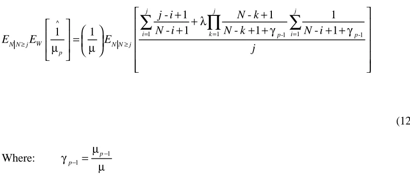
(12)

1 1

Where: γ µ

µ

− − =

p p

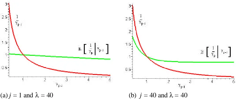
We cannot obtain a closed form solution to this equation. However, a numerical solution can be easily obtained, which shows (12) to be an unbiased estimator, if γp-1 is 1. Figure

2 is an illustration of the expectation of the MLE as a function of γp-1 compared with the

function 1/γp-1. The functions can be seen to intersect at γp-1 equal to 1.

The estimator obtained through the fixed-point iteration (9) is a biased estimator but the expectation is that it is drawn towards the true parameter value on every iteration. Consider Figure 2, and suppose a starting value for the iteration were chosen such that γ0

were greater than 1, then it is expected that γ1 (to be used in the next iteration) would be

greater than 1 but closer to 1 (i.e. γ1< γ0). Only in the situation where E[1/γp] is 1 is the

expectation of the iteration to remain unchanged. The same result is obtained if we consider an initial value chosen which is less than 1.

4. INTERVAL ESTIMATORS

The MLE can be expressed as a weighted sum of independent exponential random variables.

1 1 - 1

1 ^ - 1 - 1 1 µ λ µ − = − + =  _∑   _{+ +}   ₊        =

∑

j i e

W N i

j

We can consider the expression involving λ as the expected number of faults remaining in the system and obtain the following approximation:

^ 1 1 - 1 - 1 1 µ = =  + + _ ≥ _    +    ≈ ≈

∑

∑

j i E N N j

W N i j W j (13)

The weighted sum expressed in (13) is approximately the average of j independently and identically distributed exponential random variables and as such the distribution of the MLE is approximately Gamma distributed with mean and variance:

The approximate mean (14) is equal to the actual mean and the approximate variance is the limiting variance as we realise all the faults within the system (in addition to the limiting variance as λ approaches infinity). From (12) it is clear that the ratio of the MLE to µ, i.e. γ , is not strictly a pivotal quantity but should be approximately.

Asymptotically, the relative log-likelihood function has a Gamma distribution [26] and as such we conducted an extensive simulation exercise to investigate this property for small sample sizes. Specifically, we compared the distribution of (15) with a χ2 having 1 degree of freedom.

( )

(

)

(

)

( )

(

)

(

)

( )

(

)

exp - - '

- ! !

2 ln 2 ln

exp -!

exp - - '

- ! !

exp - exp '

2 ln

exp

-λ λ

µ µ µ

µ

λ λ

µ µ µ µ

µ µ λ µ

µ µ ∞ = = ∞ = = = =       _{ − }     _{   }   − = − _{ }      _{ } _{ − }  _{ } _   _   _{   }  _{+ −}      = −

∑

∑

∑

∑

∑

∑

n j i

n j

j

i

n j i

j j i i j j i i n

t n j t

L t _{n j n}

n

L t _{t n j t}

n j n

t t t

(

)

2 ln 2 2 exp ' exp '

λ µ

µ _{µ µ λ µ µ}

µ =        _{  } + −      _{  }     _{     }   = _{ }+ _ − _ + _{ }− _− − _        

∑

j t t t

(15)

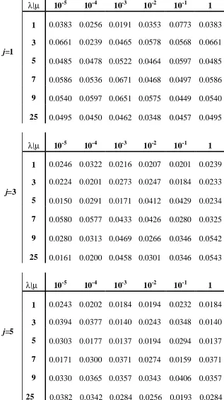
to 1, 3, 5, 7 and 9. 1000 simulations were conducted for each combination. Described within Table 1 are the maximum absolute deviations the empirical distributions from the simulations had compared with χ2 with 1 degree of freedom.

The results of the exercise showed no major difference in the maximum deviation through changing µ or λ. On average the maximum deviation decreases as the number of faults detected (i.e. j) increases. In addition, a Kolmogorov-Smirnov test [28] was used to assess the goodness-of-fit of the χ2 with 1 degree of freedom to the simulation results. We found that 78% of the 168 simulations indicate a good fit at the 5% significance level and 89% are good fits at the 1% significance level. Removing the situation where we have only one fault detected, i.e. j = 1, only 1 of the remaining 132 sets of simulations fail at the 1% significance level.

TABLE 1

5. EXAMPLE

The example is based around the context and data from the reliability growth test of a complex electronic system. While a synthetic version of the data is presented here this does not detract from the key issues arising and the way in which they are treated.

During test four faults were detected. None by 500h. Three between 500h and 1000h and a further one in a subsequent 500h of test. Numerous no fault found failures were also identified and later attributed to a particular external test problem.

At each of the review points, the Bayes OS model was applied and a selection of key results obtained.

Figure 3a shows the prior distribution elicited from the engineers. Figure 3b shows the posterior distribution with 95% confidence intervals, updated in light of the faults that were detected. Not surprisingly, the average number of faults that remain undetected in the system design decreases as test exposure increases. The prior and posterior distribution is Poisson and the time of realising these faults was modelled with an exponential distribution.

FIGURE 3

The confidence intervals in Figure 3b are obtained through the method describe in section 4 using the relative log-likelihood function to obtain confidence intervals for µ.

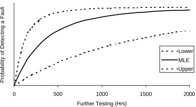
test. While the point estimate of the probability of detecting a fault within the next 1000 hours of testing was felt to be satisfactory, the lower bound of this function was not. This supported the decision to increase the stress levels of the testing in order to induce the faults that were believed to exist within the design.

FIGURE 4

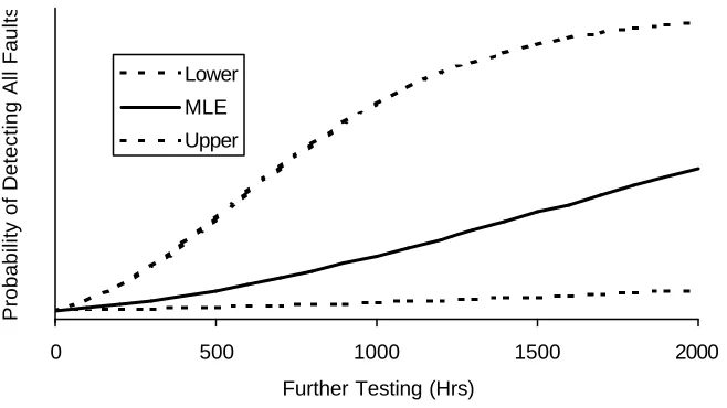
Figure 5 shows the estimate of the probability of detecting all faults that remain within the system by specified further testing time. The asymmetry in the confidence intervals is interesting, as it supports a more optimistic view of the design.

FIGURE 5

REFERENCES

[1] Z. Jelinski and P. Moranda, “Software reliability research”. Statistical Computer Performance Evaluation (ed. W. Freiberger), Academic Press, New York, 1972, pp 485-502.

[2] B. Littlewood and J.L. Verrall, “A Bayesian reliability growth model for computer software”, Appl Stat, vol. 22, 1973, pp 332-346.

[3] J.D. Musa, “A theory of software reliability and its applications”, IEEE Transactions on Software Engineering, vol. 1, part 3, 1975, pp 312-327.

[5] G.J. Schick and R.W. Wolverton, “An analysis of competing software reliability models”, IEEE Transactions on Software Engineering, vol 4, 1978 pp. 104-120. [6] B. Littlewood, “Stochastic reliability growth: A model for fault removal in computer

progams and hardware designs”, IEEE Transactions on Reliability, vol R-30, 1981, pp 313-320.

[7] R. Meinhold and N.D. Singpurwalla, “Bayesian analysis of a commonly used model for describing software failures”, The Statistician, vol 32, 1983, pp 168-173.

[8] W. Jewell, “Bayesian extensions to a basic model of software reliability”, IEEE Transactions on Software Engineering, vol 11, 1985, pp 1465-1471.

[9] F.W. Scholtz, “Software reliability modeling and analysis”, IEEE Transactions on Software Engineering, vol 12, 1986, pp 25-31.

[10] A. Csenski, “ Bayes predictive analysis of a fundamental software reliability model”, IEEE Transactions on Reliability, vol R-39, 1990, pp 177-183.

[11] J.M. Cozzolino, “Probabilistic models of decreasing failure rate processes”, Naval Research Logistics Quarterly, vol 15, 1968, pp 361-374.

[12] L.H. Crow, “Reliability analysis of complex repairable systems” Reliability and Biometry, Ed. F. Proschan and R.J. Serfling, SIAM. 1974.

[13] W.A. Jewell, “General framework for learning curve reliability growth models”, Operations Research, Vol 32, No. 3, 1984, pp 547-558.

[14] D. Robinson and D. Deitrich, “A new nonparametric growth model”, IEEE Transaction on Reliability, vol R-36, 1987, pp. 411-418.

[16] N. Ebrahimi, “How to model reliability growth when times of design modifications are known”, IEEE Transactions on Reliability, vol R-45, 1996, pp 45-58.

[17] R. Calabrai, M. Guida, and G. Pulcini, “A reliability growth model in a Bayes-decision framework”, IEEE Transactions on Reliability, vol R-45, 1996, pp. 505-510. [18] L. Walls and J. Quigley, “Learning to improve reliability during system

development”, European Journal of Operational Research, vol119, 1999, pp. 495-509.

[19] E.H. For man and N.D. Singpurwalla, “An empirical stopping rule for debugging and testing computer software”, Journal of American Statistical Association, vol 72, 1977, pp 750-757.

[20] L. Walls and J. Quigley, “Eliciting prior distributions to support Bayesian reliability growth modelling – theory and practice”, Reliability Engineering and System Safety, vol 74, 2001, pp117-128.

[21] H. Panjer and G. Willmot, Insurance Risk Models, Society of Actuaries 1992.

[22] J. Quigley and L. Walls, “Measuring the effectiveness of reliability growth testing”, Quality and Reliability Engineering International, vol 15, 1999, pp 87-93.

[23] D. London, Survival Models and Their Estimation, Actex Publications 1988. [24] R. Burden and J. Faires, Numerical Analysis, PWS Kent 1989.

[25] J. Quigley, Managing information from a reliability growth development programme, unpublished PhD thesis, University of Strathclyde, 1998.

BIOGRAPHIES John Quigley, PhD

Department of Management Science University of Strathclyde

Glasgow G1 1QE, SCOTLAND Email: [email protected]

John Quigley earned a BMath (1993) in Actuarial Science from the University of Waterloo, Canada and a PhD (1998) from the Department of Management Science, University of Strathclyde, Scotland. Currently, he is a lecturer with research interests in applied probability modeling, statistical inference and reliability growth modeling. He is also a Member of the Safety and Reliability Society, a Fellow of the Royal Statistical Society and an Associate of the Society of Actuaries.

Lesley Walls, PhD, CStat

Department of Management Science University of Strathclyde

Glasgow G1 1QE, SCOTLAND Email: [email protected]

Figure 1 Region where likelihood function is bimodal.

(a) j = 1 and λ = 40 (b) j = 40 andλ = 40

Table 1 Maximum absolute deviations of simulations from χ2 (1)

λ\µ 10-5 10-4 10-3 10-2 10-1 1

1 0.0383 0.0256 0.0191 0.0353 0.0773 0.0383 3 0.0661 0.0239 0.0465 0.0578 0.0568 0.0661

j=1

5 0.0485 0.0478 0.0522 0.0464 0.0597 0.0485 7 0.0586 0.0536 0.0671 0.0468 0.0497 0.0586 9 0.0540 0.0597 0.0651 0.0575 0.0449 0.0540 25 0.0495 0.0450 0.0462 0.0348 0.0457 0.0495

λ\µ 10-5 10-4 10-3 10-2 10-1 1

1 0.0246 0.0322 0.0216 0.0207 0.0201 0.0239 3 0.0224 0.0201 0.0273 0.0247 0.0184 0.0233

j=3

5 0.0150 0.0291 0.0171 0.0412 0.0429 0.0234 7 0.0580 0.0577 0.0433 0.0426 0.0280 0.0325 9 0.0280 0.0313 0.0469 0.0266 0.0346 0.0542 25 0.0161 0.0200 0.0458 0.0301 0.0346 0.0543

λ\µ 10-5 10-4 10-3 10-2 10-1 1

1 0.0243 0.0202 0.0184 0.0194 0.0232 0.0184 3 0.0394 0.0377 0.0140 0.0243 0.0348 0.0140

j=5

λ\µ 10-5 10-4 10-3 10-2 10-1 1

3 0.0418 0.0259 0.0199 0.0218 0.0218 0.0217

j=7

5 0.0281 0.0255 0.0219 0.0201 0.0201 0.0239 7 0.0232 0.0361 0.0167 0.0333 0.0333 0.0134 9 0.0320 0.0265 0.0333 0.0328 0.0328 0.0521 25 0.0202 0.0337 0.0265 0.0394 0.0394 0.0359

λ\µ 10-5 10-4 10-3 10-2 10-1 1 3 0.0156 0.0286 0.0339 0.0238 0.0334 0.0175

j=9

(a) Prior distribution (b) Posterior distribution with 95% confidence intervals

Figure 3 Prior and posterior distribution for the number of faults remaining undetected within the system

0 1 2 3 4 5 6 7 8 9 10 Number of Faults in System

Probability

0 1 2 3 4

Number of Faults Remaining in System

Probability Lower Bound

0 500 1000 1500 2000

Further Testing (Hrs)

Probability of Detecting a Fault

Lower

MLE

Upper

0 500 1000 1500 2000

Further Testing (Hrs)

Probability of Detecting All Faults

Lower

MLE

Upper