Rochester Institute of Technology
RIT Scholar Works
Theses
Thesis/Dissertation Collections
2010
Practical programming with total functions
Karl Voelker
Follow this and additional works at:
http://scholarworks.rit.edu/theses
This Thesis is brought to you for free and open access by the Thesis/Dissertation Collections at RIT Scholar Works. It has been accepted for inclusion in Theses by an authorized administrator of RIT Scholar Works. For more information, please [email protected].
Recommended Citation
Practical Programming with Total Functions
Karl Voelker
July 27, 2010
Submitted in fulfillment of the requirements for the degree of Master of Science.
Department of Computer Science
Golisano College of Computing and Information Sciences Rochester Institute of Technology
Rochester, New York
Chair, Professor Matthew Fluet
Reader, Professor James Heliotis
Observer, Professor Stanis law P. Radziszowski
Abstract
Contents
1 Background 1
1.1 Implementing a Total Language . . . 2
1.2 Codata and Corecursion . . . 4
1.3 Numbers in TFP . . . 5
2 Summary of Work 8 2.1 The Compiler . . . 8
2.2 The Libraries . . . 8
2.3 The Examples . . . 9
3 The Compiler 10 3.1 The Sound Recursion Rule . . . 10
3.1.1 My Rule . . . 12
3.1.2 Other Considered Rules . . . 20
3.2 The Productive Corecursion Rule . . . 22
3.2.1 Turner’s Rule . . . 22
3.2.2 My Rule . . . 23
3.3 Mixed Recursive-Corecursive Cycles . . . 23
3.4 Other Interactions with Haskell and GHC . . . 23
3.4.1 With Haskell 98 . . . 24
3.4.2 With GHC . . . 26
3.5.1 Location in the Compilation Pipeline . . . 28
3.5.2 The Implementation of Codata . . . 29
3.5.3 Use of Language Options . . . 30
3.5.4 Use of Annotations . . . 30
4 The Libraries 31 4.1 Natural Number Types . . . 31
4.2 Simple Changes to Haskell 98 Functions . . . 33
4.3 Changes to Haskell 98 Classes . . . 34
4.4 TheTotal.Data.CoList Library . . . 35
4.4.1 Generalizing Lists and Colists . . . 36
4.4.2 Functions Borrowed fromData.List . . . 37
4.4.3 New Functions . . . 38
4.4.4 Missing Functions . . . 39
4.5 TheTotal.Data.MapLibrary . . . 40
4.6 TheTotal.Data.Array Library . . . 41
4.7 The I/O Libraries . . . 41
4.7.1 Simple I/O: Standard Input and Output . . . 42
4.7.2 I/O with Files: Two Approaches . . . 43
4.7.3 Three Practical Paradigms . . . 45
4.7.4 ImplementingTotal.IO . . . 46
4.7.5 Filesystem Navigation . . . 50
5 The Examples 52 5.1 Calculator . . . 52
5.1.1 Making the Induction More Exact . . . 55
5.1.2 Alternate Approaches to Parsing . . . 56
5.2 Regular Expressions . . . 56
5.3 Sudoku Solver . . . 58
5.4 A* Search . . . 61
5.6 Robot Simulator . . . 63
5.7 File Finder . . . 64
5.8 Text Searcher . . . 64
6 Lessons Learned 65 6.1 Programming Techniques . . . 65
6.1.1 More and Simpler Algorithms . . . 65
6.1.2 Resorting to an Inexact Induction Variable . . . 66
6.1.3 Relying on Lazy Evaluation . . . 67
6.2 Numeric Type Classes . . . 68
6.3 Walther Recursion . . . 69
6.3.1 Usefulness . . . 71
7 Future Work 73 7.1 The Total Language . . . 73
7.1.1 Walther Recursion and Beyond . . . 73
7.1.2 Identifying Induction Variables . . . 74
7.1.3 Natural Number-Typed Induction Variables . . . 75
7.1.4 List Literals and Comprehensions . . . 75
7.2 Implementation of Type Classes . . . 76
7.3 Generalizing Over Codata Types . . . 76
7.4 The Total Prelude . . . 76
8 Related Work 77 8.1 Agda . . . 78
8.2 Epigram . . . 78
8.3 Relationship to Walther Recursion . . . 79
List of Figures
3.1 Turner’s Rule . . . 11
3.2 Mutually-recursive cycles . . . 13
3.3 My initial rule . . . 14
3.4 My initial rule, with partial application . . . 14
3.5 My initial rule, with partial application and nested functions . . 16
3.6 My final rule . . . 17
3.7 My final rule, continued . . . 18
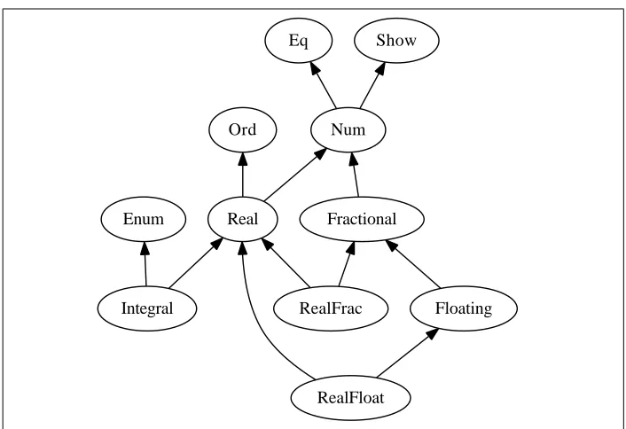
6.1 Haskell 98 numeric type classes and their parents . . . 69
Chapter 1
Background
Functional programming (FP) languages are known for their great expressive power. Even better, by allowing—or, in the case of pure FP, mandating— a referentially-transparent programming style, reasoning about the behavior of such programs is made easier. This is advantageous to students who are learning to write programs, because they can easily work out what their programs are doing, and they can think in the mathematical terms they’ve already learned.
For example, consider two functions which sum the numbers in a list:
sum :: [ Int ] -> Int
sum [] = 0
sum ( x : xs ) = x + sum xs
int sum ( int n , int * arr ) {
int acc = 0;
for ( int i = 0; i < n ; ++ i ) {
acc += arr [ i ];
}
return acc ;
The first function, written in Haskell, can be understood via equational reasoning, a process fundamentally comprehensible to anyone who has studied basic algebra, which looks like this:
sum([2,3]) = 2 +sum([3]) = 2 + 3 +sum([]) = 2 + 3 + 0 = 5
Equational reasoning does not suffice for the second function, written in C. Understanding how the C function computes the sum requires understanding the imperative model of a program as a sequence of steps and the concept of rewritable computer memory.
Unfortunately, even a pure functional program can encounter a run-time error, such as dividing by zero or taking the head of an empty list, and even a pure functional program may fail to terminate. It can thus be said that many of the functions in such a program arepartial functions. Furthermore, if all the functions in a program weretotal rather than partial, run-time errors and non-termination would be impossible. Of course, deciding the totality of a function is, in general, an undecidable problem.
Despite the impossibility of the problem when applied to the language of all functions, it is entirely feasible to define a more restrictive language in which all functions happen to be total. Programs written in such a language would have many desirable properties: they could not encounter run-time errors or infinite loops, theorems about their meaning could be more easily proven, including by automated provers, and as such they could be more aggressively optimized and analyzed by compilers.
1.1
Implementing a Total Language
rules are:
• All data must be immutable.
• All pattern-matching must be exhaustive, since clearly any function which employs non-exhaustive pattern-matching must not be total.
• Datatype definitions must not recurse on the left-hand side of an → op-erator. Types violating this rule can allow arbitrary recursion to sneak back into the language via the creation of a fixpoint operator, as in this example [30]:
data F a b = F ( F a b -> a -> b )
fix :: ( F a b -> a -> b ) -> ( a -> b )
fix f = f ( F f )
up :: Int -> Int
up = fix (\( F f ) a -> f ( F f ) ( a + 1))
• Recursion must be structural. Thus, all recursive calls must be made by “syntactic descent on data constructors.” This is also known as “primitive recursion.” An example is this definition ofmap:
map :: ( a -> b ) -> [ a ] -> [ b ]
map f [] = []
map f ( x : xs ) = f x : map f xs
In that example, whenmapis called on a non-empty list, (x : xs), the recursive call is made on xs, which is known by the use of deconstruc-tor syntax to be a subcomponent of(x : xs). Conceptually, requiring structural recursion allows the compiler to infer a proof by induction of the recursive function’s termination. As such, the second parameter of
l o g 2 _ a p p r o x 1 = 0
l o g 2 _ a p p r o x n = 1 + l o g 2 _ a p p r o x ( n ‘ div ‘ 2)
That example is invalid because, when log2 approx is called on n, the recursive call is made on⌊n
2⌋, which is not the direct result of any use of
deconstructor syntax onn.
1.2
Codata and Corecursion
If a language were limited entirely to structurally recursive functions or Walther recursive functions [20] (described further in Section 6.3), it would be able to express many useful algorithms, but would not be well-suited to the implemen-tation of operating systems, which may be intended to run forever. As such, Turner suggests that in addition to data and functions, which are necessarily finite, a language should also provide codata and cofunctions, which are poten-tially infinite. [30]
Codata constructors are defined in the same manner as data constructors. A cofunction is one which produces a result of a codata type. If a cofunction recurses, that corecursive call must be directly wrapped by a coconstructor call. This ensures that although a codata structure may be infinite, the computation needed to reach down one layer into the structure is always finite. Cofunctions meeting this criterion are described as “productive.”
Although codata appear syntactically similar to data, one important dif-ference is that recursing on the substructure of a codata value does not make recursion valid, since in an infinite codata structure, a substructure is no closer to the “bottom” than the structure which contained it.
Turner suggests two possible uses of codata with little elaboration [30]:
• A language may provide input and output facilities via special codata structures. A simple approach similar to that used by Miranda [19] is to have each input stream represented by aColist Char. If an earlier part of the colist is read a second time, the data will be provided from a cache so that it is guaranteed to match what was read the first time.
• A program may represent infinite concepts, such as the Fibonnaci se-quence, directly.
Consider this simple example borrowed from Turner [30]:
codata Colist a = Nil | Cons a ( Colist a )
comap :: ( a -> b ) -> Colist a -> Colist b
comap _ Nil = Nil
comap f ( Cons h t ) = Cons ( f h ) ( comap f t )
In the example above, the corecursive call to comapis an argument to the coconstructorCons. In contrast, consider this unfortunately invalid example, also borrowed from Turner [30]:
evens = Cons 2 ( comap (+ 2) evens )
This example is invalid because the corecursive call toevensis not directly wrapped in a coconstructor due to the intervening call tocomap. Despite not being regarded as valid, evensis nonetheless productive. Telford and Turner describe an abstract interpretation which would allow this definition ofevens. [27] Implementing that abstract interpretation would be a significant effort on its own, and as such is beyond the scope of this work.
1.3
Numbers in TFP
Pro-gramming suggests that any such language should include a type for natural numbers. Runciman suggests that natural numbers should be given greater weight in any programming language, as well as giving rationale for certain def-initions of arithmetic operations on the natural numbers. [24] Some features of the given definitions are:
• 0−n= 0
The rationale for this definition is an analogy to the concrete situations these numbers frequently represent. One concrete example is a list. Con-sider this typical definition ofdrop:
drop _ [] = []
drop 0 xs = xs
drop ( n + 1) ( x : xs ) = drop n xs
Combining drop with the given definition of subtraction, we have the identitylength (drop n xs) == (length xs) - n.
• n
0 =n
The rationale for this definition is based on another function defined by Runciman, slice(n, d) = n
d+1. [24] This function can be understood as
finding the size of one slice of nwhen dcuts are made. Division is then defined as div(n, d) = slice(n, d−1). So, when d > 0, div(n, d) = n
d, but when d = 0, div(n,0) = slice(n,0 −1) = slice(n,0) = n
1 = n,
using the aforementioned definition of subtraction. It is noted that this definition of division is monotonic, but no more practical suggestions are made regarding its value.
An alternative to this kind of division, also mentioned by Runciman, is to use n
0 =∞. Although infinity is often represented with a special data
Chapter 2
Summary of Work
2.1
The Compiler
I adapted Turner’s rules for sound recursion and productive corecursion [30] to the complex Haskell 98 language. Then, inside the Glasgow Haskell Compiler (GHC), version 6.12, a popular Haskell compiler, I implemented the adapted rules. The rules are enabled by a GHC “language option” so that the compiler can be used normally or in “total mode,” in which case a total module is pro-duced. In addition to implementing the rules, I also added codata declarations to the input syntax accepted by GHC in total mode.
2.2
The Libraries
I adapted the Haskell standard libraries, and some important libraries included with GHC, to only expose total functions. This was accomplished partly by exporting existing safe functions, partly by implementing wrappers to make existing functions safe, and partly by writing completely new functions.
2.3
The Examples
Chapter 3
The Compiler
3.1
The Sound Recursion Rule
The rule described by Turner requiring structural recursion [30] is simple, so simple that no formalized description was necessary to make it clear. My work in the context of Haskell [11], a much more complicated language, has produced a rule which demands a formal description.
I will begin by formalizing Turner’s rule, Figure 3.1, so that I may formalize mine in the same terms. All of the formalizations in this chapter operate on syntactic entities, primarily named function definitions. Also, at the stage in the compiler where the rule is implemented, all variables have been given unique identifiers, so two mentions of a variable are equal iff they mention the same variable.
Note that in Figure 3.1, the function u, which identifies the bindings that result from pattern-matching deconstruction of a parameter, returns bindings regardless of their depth in the structure of the pattern. For example, consider this function:
f ( x1 : ( x2 : xs )) = xs
The predicatepis the critical component of Figure 3.1. A rough explanation of the meaning ofpis that, among the arguments to a recursive call:
• one argument must be a substructure of the corresponding input param-eter, and
• all preceding arguments must either be substructures of or equivalent to their corresponding input parameters.
Letn(f) be the arity off.
Leta(f, i) be theith parameter binding off fori∈[0, n(f)).
Letu(f, i) be the set of all bindings made by case analysis ona(f, i) in patterns of the formD X∗, where Dis a data constructor andX is a pattern.
Letr(f) be the number of recursive applications off.
Let g(f, i, j) be the ith argument of the jth recursive application of f for
j∈[0, r(f)) andi∈[0, n(f)).
Letp(f) be true iff∀j∈[0, r(f)) ∃i∈[0, n(f)) such that: – g(f, i, j)∈u(f, i) and
– ∀h∈[0, i) [g(f, h, j) =a(f, i)]. A functionf follows Turner’s rule iffp(f).
Figure 3.1: Turner’s Rule
The meaning of Turner’s rule can be demonstrated with an example. We will consider two functions, one valid and one invalid. To imitate the abstract syntax upon which the rule is actually executed, each binding has a unique name and pattern-matching is only done incaseexpressions.
f :: [ Int ] -> [ Int ]
f xs = case xs of
[] -> 0
g :: [ Int ] -> [ Int ]
g ys = 1 : g ys
Now, let us trace the evaluation of the rule on these examples step by step:
n(f) = 1
a(f,0) =xs
u(f,0) ={x,xs′} r(f) = 1
g(f,0,0) =xs′ g(f,0,0)∈u(f,0)
p(f)
n(g) = 1
a(g,0) =ys
u(g,0) =∅
r(g) = 1
g(g,0,0) =ys
g(g,0,0)∈/u(g,0)
¬p(g)
3.1.1
My Rule
I will first present a basic form of my rule for recursion, Figure 3.3, followed by three important enhancements. Informally, my rule is different in that it accounts for mutual recursion, a feature of Haskell 98.
Mutual recursion is handled by the rule that in any mutually-recursive cycle of functions, there must be one function in which all calls to any functions in the cycle follow Turner’s rule as if those were directly recursive calls. This is the first part ofp(c), which begins with∃f ∈c.
Furthermore, all other functions in the cycle must follow a slightly looser rule: rather than having to descend on the structure of their arguments, they must merely not expand the structure of their arguments. This is the second part ofp(c), which begins with∀f ∈c.
Mutual recursion between functions of differing arity must also be consid-ered. In the rule, we find the minimum arity of all functions in a cycle (n′(c))
p
x
y
z
f
g
[image:20.612.129.482.121.318.2]h
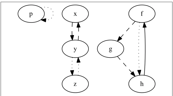
Figure 3.2: Mutually-recursive cycles: each cycle in a graph is drawn in a distinct style, with a solid edge being in all the graph’s cycles.
The rule does not formally define what a mutually-recursive cycle is, but I will give a definition here: a mutually-recursive cycle is a cycle in the static call graph which does not visit any function more than once. A mutually recursive cycle may consist of a single function which calls itself. This isn’t really “mutual recursion,” but that doesn’t matter for the purposes of these rules. Figure 3.2 contains some example cycles.
Partial Application
Extending Turner’s rule to support partial applications, a feature of Haskell 98, is trivial. The only real problem with the formal rule as written is that the definition ofpmay go out-of-bounds in its use ofg.
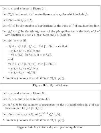
Letn,a, andube as in Figure 3.1.
LetC(f) be the set of all mutually-recursive cycles which includef. Letn′(c) = min
f∈cn(f).
Letr(f, c) be the number of applications in the body off of any function inc.
Letg(f, c, i, j) be the ith argument of thejth application in the body of f of
any function inc forj∈[0, r(f, c)) andi∈[0, n(f)). Letp(c) be true iff:
– ∃f ∈c ∀j∈[0, r(f, c)) ∃i∈[0, n′
(c)) such that: – g(f, c, i, j)∈u(f, i) and
– ∀h∈[0, i) [g(f, c, h, j) =a(f, i)]. and
– ∀f ∈c ∀j∈[0, r(f, c)) ∀i∈[0, n′(c)):
– g(f, c, i, j)∈u(f, i) or – g(f, c, i, j) =a(f, i).
A functionf follows this rule iff∀c∈C(f) [p(c)].
Figure 3.3: My initial rule Letn,a, andube as in Figure 3.1.
LetC,r,g, andpbe as in Figure 3.3.
Let s(f, c, j) be the number of arguments to thejth application in f of any
function incforj ∈[0, r(f, c)). Letn′(c) = min
f∈c{n(f),min r(f,c)−1
j=0 s(f, c, j)}.
[image:21.612.130.483.106.571.2]A functionf follows this rule iff∀c∈C(f) [p(c)].
Figure 3.4: My initial rule, with partial application
Nested Functions
f xs = g xs
where
g xs = g xs
Treating nested functions the same as top-level functions gives a sound rule, but one which is excessively restrictive, as demonstrated by this example:
f [] = []
f xss@ ( xs : xss ’) = g xs
where
g [] = f xss ’
g ( x : xs ’) = x + g xs ’
The problem with this example is thatxss’is not related to any parameter ofg, so the callf xss’in gis invalid, according to the rules developed so far.
This example could easily be rewritten to follow the rule. This example may even seem pointless. However, GHC routinely generates code of roughly this form in its desugaring phase, and my implementation of this rule comes after that phase, so accepting functions of this form is critical for my implementation. The rule that supports nested functions is Figure 3.5.
The solution to the problem of nested functions is simply to observe that a nested function can utilize all the parameters of its enclosing functions as if they were its own parameters. As such, the nested function rule uses a function
w(f), the function in which f is nested, in numerous recursive definitions. For example, a(f, i), the ith parameter of f, now recurses on w(f) in order to treat the parameters ofw(f) as parameters off. Other parts of the rule have undergone a similar transformation.
Unfortunately, there is one remaining problem with this rule which prevents the functionfin the example above from being accepted. The problem is that
n′({
f,g}) = 1 because n(f) = 1. The rule effectively rewrites the application
g xs’ to be g xss xs’, and since n′({
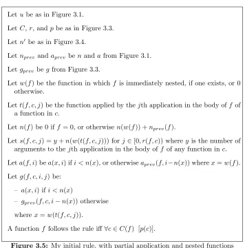
Letube as in Figure 3.1.
LetC,r, andpbe as in Figure 3.3. Letn′ be as in Figure 3.4.
Letnprev andaprevbe nandafrom Figure 3.1. Letgprev beg from Figure 3.3.
Letw(f) be the function in whichf is immediately nested, if one exists, or 0 otherwise.
Lett(f, c, j) be the function applied by thejth application in the body off of
a function inc.
Letn(f) be 0 iff = 0, or otherwisen(w(f)) +nprev(f).
Lets(f, c, j) =y+n(w(t(f, c, j))) forj∈[0, r(f, c)) wherey is the number of arguments to thejth application in the body off of any function inc. Leta(f, i) bea(x, i) ifi < n(x), or otherwiseaprev(f, i−n(x)) wherex=w(f). Letg(f, c, i, j) be:
– a(x, i) ifi < n(x)
– gprev(f, c, i−n(x)) otherwise wherex=w(t(f, c, j)).
[image:23.612.128.484.115.475.2]A functionf follows the rule iff∀c∈C(f) [p(c)].
Figure 3.5: My initial rule, with partial application and nested functions
Parameter Permutations
Letw(f) be the function in whichf is immediately nested, if one exists, or 0 otherwise.
Letn(f) be 0 iff = 0 orn(w(f)) +xotherwise, wherexis the arity off. Leta(f, i) fori∈[0, n(f)) be:
– a(x, i) ifi < n(x)
– theyth parameter binding off otherwise, wherey=i−n(x). wherex=w(f).
Letu(f, i) be the set of all bindings made by case analysis ona(f, i) in patterns of the formD X∗, where Dis a data constructor andX is a pattern.
Letr(f, c) be the number of applications in the body off of any function inc. LetC(f) be the set of all mutually-recursive cycles which includef.
Lets(f, c, j) =y+n(w(t(f, c, j))) forj∈[0, r(f, c)) wherey is the number of arguments to thejth application in the body off of any function inc. Letn′(c) = min
f∈c{n(f),min r(f,c)−1
j=0 s(f, c, j)}.
Note that n′(c)≥min
f∈c{n(w(f))}.
Lett(f, c, j) be the function applied by thejth application in the body off of
[image:24.612.130.485.101.458.2]a function inc.
Figure 3.6: My final rule, continued in Figure 3.7
number of parameters so that checking all permutations can be done in only a few seconds.
In the case of mutually recursive cycles, it is necessary to check all ways in which one permutation can be taken for each of the functions in the cycle.
My implementation first calculates the number of permutations which will have to be considered to do an exhaustive search. If that number is beyond a limit, no permutations are considered other than the one which appears in the program as written. After some experimentation, the limit was set at 7!2 =
25,401,600, enough for a mutually recursive cycle of two functions, each of which has seven arguments.
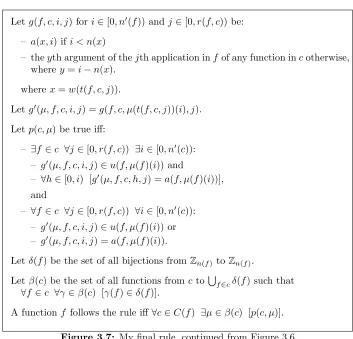
Letg(f, c, i, j) fori∈[0, n′(f)) andj∈[0, r(f, c)) be:
– a(x, i) ifi < n(x)
– theyth argument of thejth application inf of any function incotherwise, wherey=i−n(x).
wherex=w(t(f, c, j)).
Letg′(µ, f, c, i, j) =g(f, c, µ(t(f, c, j))(i), j).
Letp(c, µ) be true iff:
– ∃f ∈c ∀j∈[0, r(f, c)) ∃i∈[0, n′
(c)): – g′(µ, f, c, i, j)∈u(f, µ(f)(i)) and
– ∀h∈[0, i) [g′(µ, f, c, h, j) =a(f, µ(f)(i))],
and
– ∀f ∈c ∀j∈[0, r(f, c)) ∀i∈[0, n′(c)):
– g′(µ, f, c, i, j)∈u(f, µ(f)(i)) or
– g′(µ, f, c, i, j) =a(f, µ(f)(i)).
Letδ(f) be the set of all bijections fromZn(f)to Zn(f).
Letβ(c) be the set of all functions fromc toSf∈cδ(f) such that
∀f ∈c ∀γ∈β(c) [γ(f)∈δ(f)].
[image:25.612.128.481.115.454.2]A functionf follows the rule iff∀c∈C(f) ∃µ∈β(c) [p(c, µ)].
Figure 3.7: My final rule, continued from Figure 3.6
3.5). I will later discuss some possible rules which I have not implemented. It seems likely that there is a more efficient algorithm for solving this problem than a brute-force search of all permutations.
Now, consider these example functions:
-- correct
f :: [ Int ] -> [ Int ] -> Int
f xs ys = g xs ys where
g ms ns = case ms of
[] -> case ns of
[] -> 0
( m : ms ’) -> m + g ms ’ ns
-- i n c o r r e c t
f :: [ Int ] -> [ Int ] -> Int
f xs ys = g xs ys where
g ms ns = case ms of
[] -> case ns of
[] -> 0
( n : ns ’) -> n * g xs ns -- typo
( m : ms ’) -> m + g ms ’ ns
The first definition offis correct. The second definition is almost the same, but contains a typo which invalidates it. Now, we will see, step by step, how my complete rule, as implemented, is applied to these functions.
Facts common to both definitions
w(f) = 0 w(g) =f n(f) = 2 n(g) = 4
a(f,0) =a(g,0) =xs a(f,1) =a(g,1) =ys
a(g,2) =ms a(g,3) =ns
u(f,0) =u(f,1) =u(g,0) =u(g,1) =∅
u(g,2) ={m,ms′}
u(g,3) ={n,ns′}
C(f) =∅ C(g) ={{g}}
Letc={g}, noting thatC(g) ={c}.
s(g, c,0) =s(g, c,1) = 4 t(g, c,0) =t(g, c,1) =g
r(g, c) = 2 n′(
g) = 4
g(g, c,0,0) =g(g, c,0,1) =a(f,0) =xs
g(g, c,2,0) =xs
g(g, c,2,1) =ms′ g(
g, c,3,1) =ns
Facts about correct definition
g(g, c,3,0) =ns′
Facts about incorrect definition
g(g, c,3,0) =ns(the typo)
Now, note that|δ(g)|= 4! = 24 andc={g}, so|β(c)|= 24. To show that the correct definition of fis valid, it must be shown that ∃µ∈ β(c) [p(c, µ)]. However, to show that the incorrect definition offis invalid, it must be shown that ∀µ ∈ β(c) [¬p(c, µ)]. This would be more tedious than enlightening, so instead I will only show that the one particular value ofµwith which I validate the correct definition offdoes not validate the incorrect definition off.
Facts common to both definitions
Letµ(g) =λn.3−n.
g′(µ,
g, c,3,0) =g′(µ,
g, c,3,1) =a(f,0) =xs
g′(µ,
g, c,2,0) =g′(µ,
g, c,2,1) =a(f,1) =ys
g′
(µ,g, c,1,0) =xs
g′(µ,
g, c,1,1) =ms′∈u(
g,2) g′(µ,
g, c,0,1) =ns=a(g,3)
Facts about correct definition
g′
(µ,g, c,0,0) =ns′ g′
(µ,g, c,0,0)∈[u(g,3) ={n,ns′}
]
p(c, µ)
Facts about incorrect definition
g′
(µ,g, c,0,0) =ns(the typo)
∀i∈[0,3] [g′
(µ,g, c, i,0)∈/ u(g,3−i)]
¬p(c, µ)
3.1.2
Other Considered Rules
However, since these cases have not arisen in practice, and accounting for them may increase the cost of checking adherence to the rule, it’s possible that they are not worth implementing.
First, consider this example:
foo 0 x = x
foo ( n +1) x = bar n ( x +1)
bar n x = foo n ( x +1)
Letf =bar. Thus,C(f) ={{foo,bar}}. Letc={foo,bar}. Thus we have:
• n′(c) = 2
• g(f, c,0,0) =n
• g(f, c,1,0) =(x+1)
• ∀µ∈β(c),∃i∈ {0,1} such that:
– g′(µ, f, c, i,0)∈/u(f, µ(f)(i)) and
– g′(µ, f, c, i,0)6=a(f, µ(f)(i))
Thus,∀µ∈β(c),¬p(c).
Informally, the problem is that my rule blindly looks at both arguments in both applications. In the application offoo, that’s a problem: if only the first argument had been considered, the rule would have recognized that it was the same as the input, but when considering both arguments, the arguments on the whole are bigger than the input.
The reason why it would be safe to only look at the first argument to the application of foo is that we only need to look at the first argument to the application of bar to discern that in that application, the arguments on the whole are smaller than the input.
all values in{1..n′(c)}. Alternately, the rule could first find all functions which
recurse on values smaller than their inputs, and then find the one which reliably does so while considering the least number of the parameters.
Note that simply picking an arbitrary function which recurses on values smaller than its input is not enough. There could be a cycle with two candidate functions, where one candidate is better than the other, such as in this example:
foo 0 x = x
foo ( n +1) x = bar n ( x +1)
bar 0 0 = 0
bar ( n +1) 0 = baz n 1
bar n ( x +1) = baz n x
baz n x = foo n ( x +2)
From looking at foo, we would decide to only consider one parameter, whereas from looking at bar, we would decide to consider two parameters, which would make the cycle be considered invalid because of the recursion in
baz.
3.2
The Productive Corecursion Rule
The goal of a rule for productive corecursion is to ensure that descending a finite depth into a recursive codata structure will not require infinite computation.
3.2.1
Turner’s Rule
3.2.2
My Rule
My rule is that a corecursive functionf is accepted iff in each cyclecof mutually corecursive functions containingf, there exists a functiong incsuch that each application ing of any function inc is an argument to a codata constructor.
3.3
Mixed Recursive-Corecursive Cycles
Having considered only briefly the possibility of mutual recursion between func-tions and cofuncfunc-tions, I simply banned them in my implementation. However, upon further reflection, it does seem that such a stringent rule is not necessary. If all the functions in a mixed cycle are judged by the standard for total recursion, the result types don’t matter: the functions terminate.
If all the functions in a mixed cycle are judged by the standard for productive corecursion, then if there are infinite recursive applications, each one is wrapped directly in a coconstructor, which is exactly where infinite data are supposed to be. No finite function can accidentally begin some nonterminating recursion by descending down this data, since the inductive inference cannot be made by pattern-matching on a coconstructor.
So, it seems that either standard can be applied to a cycle, so long as it is applied to all the functions in that cycle. Thus, the ideal check would be to check each cycle against both standards, succeeding if either subcheck succeeds. However, the need for this check never arose in my examples, which are described in Chapter 5.
3.4
Other Interactions with Haskell and GHC
3.4.1
With Haskell 98
Record Accessors
Haskell specifies a “record syntax” which can be used to make data constructors of high arity more convenient [9], but a record accessor produces a run-time error if used on a value made with the wrong data constructor [10]. Consider this example:
data T a = Foo { x :: a } | Bar { y :: a }
x :: T a -> a -- i m p l i c i t
n :: Int
n = x ( Bar { y = 3 }) -- error
The solution to this problem which I implemented is a simple check: if a data constructor uses record syntax, it must be the only constructor of its type. That way, the convenience of the record syntax is not lost in cases where it is safe.
Another solution would have been to make record accessor functions return a Maybe. It might be ideal to change record accessors in this way only when there are multiple data constructors for a type, to avoid unnecessary Maybes. Then again, this would mean that adding a data constructor to a type could break a lot of existing code.
Record Construction
Haskell’s record syntax causes further trouble in that an application of a record constructor is not required to provide values for all the fields [10]. Unmentioned fields are undefined:
data T a = Foo { x :: a }
n :: Int
n = x ( Foo { }) -- error
Type Classes
There are four ways in which Haskell’s type classes [14] interact poorly with my implementation of TFP.
First, an instance declaration is not required to implement all the methods in the class. Any methods without an implementation produce a run-time error. This behavior was simple to change in the compiler, since it already issues a warning about undefined methods.
Second, corecursive functions cannot be class methods. This is due to the prohibition of mutually-recursive cycles which mix data and codata. Such cycles arise between a corecursive method and the corresponding instance dictionary. This limitation has been problematic in only one case so far in my experiments, that being theenumFrom andenumFromThen methods of theEnum class, which produce potentially-infinite lists of values from an enumeration.
Third, methods cannot be implemented in terms of each other. This is because of recursion which arises between the instance method and the instance dictionary. Consider this example:
class Foo a where
bar :: a -> a
baz :: a -> a
i n s t a n c e Foo Int where
bar = id
baz = bar
After desugaring, the code looks roughly like this:
-- class Foo a where ...
Foo bar baz = ( bar , baz )
Foo_bar ( bar , _ ) = bar
-- i n s t a n c e Foo Int where ...
Foo_Int = Foo F o o _ I n t _ b a r F o o _ I n t _ b a z
F o o _ I n t _ b a r = id
F o o _ I n t _ b a z = Foo_bar Foo_Int
The invalid mutual recursion is betweenFoo IntandFoo Int baz.
Fourth, an instance must define all the methods of the class, even if the class provides default implementations of some methods. This problem has a cause similar to the previous one.
Modules
A Haskell program is formed from a set of modules [13]. Clearly, a total module must not import a non-total module, and this restriction is implemented. Total modules may, however, be imported by any other module. Although a non-total module may “poison” its use of a non-total module by, for example, passing an infinite list into a total function, it cannot poison the total module in any global sense because of the pure functional nature of Haskell.
Incomplete Patterns
A case analysis in Haskell is not required to be complete [10], whereas this completeness is one of Turner’s requirements [30]. I have implemented this requirement, although doing so was quite trivial, because GHC has the ability to warn about incomplete case analysis.
3.4.2
With GHC
Type Synonyms
sake. However, GHC does not do this. To some extent, this may be explainable by GHC’s support for certain extensions to the Haskell language related to the treatment of type synonyms.
Implementing Turner’s requirement that datatypes be covariant [30] was made somewhat trickier by the possible presence of type synonyms in types.
Rebindable Syntax
Standard Haskell specifies various forms of “syntactic sugar” which map onto functions from the standard libraries. The scope in which such sugar is used does not matter: the sugar always references the same, standard functions [10]. Two forms of this sugar,do-notation and enumeration sequences (..-notation), are based on classes for which the total standard libraries have substitutes:
MonadandEnum respectively. As such, I needed some mechanism by which the altered versions of these classes would be used in the desugaring process. Fortu-nately, GHC includes such a mechanism, called “rebindable syntax.” [29] With this option enabled, certain syntactic forms look for the relevant functions in their scope rather than grabbing the standard function out of nowhere.
Incompatible Language Options
GHC supports many extensions to the Haskell language [28]. Many seemed dubious within the context of TFP: either they might cause trouble for my implementation in particular, or they might provide backdoors for breaking totality in general. Proving the safety of all of GHC’s extensions is beyond the scope of this work, so those which are not obviously safe have been disabled.
3.5
Important Implementation Details
implementation.
3.5.1
Location in the Compilation Pipeline
Initially, I began to implement Turner’s sound recursion rule in the front-end of GHC, operating on the HsSyn syntax, which represents the full syntactic complexity of Haskell. However, I soon realized that adapting Turner’s rule to such a wide variety of syntactic forms, many with great semantic depth, would be a time-consuming task.
Since the original goal of this project was to put as much focus on the libraries and example programs as on the compiler, I didn’t want to become mired in work at only the first stage of the project. As such, I decided to implement Turner’s rule in the middle-end of GHC, operating on the vastly simpler core syntax.
That choice probably made my work easier, but not by as much as I had expected. Furthermore, I would highly recommend that any production-quality implementation of this concept operate at the highest syntactic level possible. The fundamental reason for this is that Turner’s check is syntactic in nature, so the more changes the syntax has undergone internally, the greater the chance that a program which ought to be valid will be transformed into one which is invalid.
Now, I continue with details about the specific problems caused by work-ing with the core syntax, as well as addresswork-ing issues which would arise when working with the rich syntax.
Poor Error Messages
messages.
n+kPatterns
Identifying uses ofn+k patterns in the core syntax is a challenge, since these patterns have disappeared and been replaced by expressions involving various arithmetic and comparison operators. My implementation looks for expressions which match the pattern generated by the compiler fromn+kpatterns.
It might have been easier to identifyn+kpatterns earlier in the compiler and record the identifiers involved for later use, but at the time it seemed that it would be more expeditious to identify the expression patterns than to acquaint myself with more gigantic portions of the GHC source code which bore little resemblance to the code with which I had already become familiar.
These patterns also cause an issue in identifying complete pattern matching. Sincen+kpatterns were originally intended for use on integral types, the com-piler correctly considers{0,n+1}to be an incomplete set of patterns, since the patternn+1only matches positive values of n, as per the specification. Yet, in the case of the natural number types, such a set of patterns is complete. No so-lution to this problem is implemented, since there is a fairly trivial workaround: put the0case last, and replace0with .
Handlingdo-Notation
In retrospect, the semantics ofdo-notation may not be as daunting for Turner’s rule as I had guessed. The only thing hidden by the notation is the use of the functions defined in theMonad class. So, except in the definition of an instance ofMonad, the applications which are missing from the syntax will not be relevant to the detection of recursion.
3.5.2
The Implementation of Codata
codata easier. In my implementation, data and codata are indistinguishable but for a Boolean flag carried by all the types which are used to describe data types in the various syntaxes, including the syntax which gets serialized into interface files.
3.5.3
Use of Language Options
GHC, as a result of its many language extensions [28], already has a system in place for enabling and disabling extensions on a per-module basis. These “language options” can be enabled and disabled on the command line or in a module file with a special pragma. My implementation uses three language options:
• Codata, which allows thecodatasyntax.
• Total, which enables checking of all the rules (and implies Codata).
• FakeTotal, which is used by certain system libraries to declare that they are believed to be total, although they should not be checked.
3.5.4
Use of Annotations
Chapter 4
The Libraries
4.1
Natural Number Types
Natural numbers, as noted by Runciman [24], are to be found everywhere in computer programs, as descriptors of the size of or a position in any finite data structure or computation. Yet, natural numbers have traditionally been ignored in favor of integers, which avoid certain fundamental problems such as how to define subtraction.
It is precisely because of the use of natural numbers to describe finite struc-tures that Runciman’s definition of 0−n= 0 makes sense. This is the definition used in my implementation.
Another important question is how natural numbers should be implemented. The “textbook” approach is to define them as any other data type:
data Natural = Zero | Succ Natural
which rely on a natural number as the induction variable.
However, the run-time efficiency of nearly any operation on this type is dismal when compared to that of a machine integer. This desire for efficiency, which in a practical context may turn out to be quite critical, can be realized with this definition:
newtype Natural a = Natural a
This type is parameterized by what integer type we wish to use as its backing. In implementing the standard numeric instances for this type, we can indicate the constraint that the backing must indeed be an integer:
i n s t a n c e ( I n t e g r a l a ) = > I n t e g r a l ( Natural a ) where
f r o m I n t e g e r = Natural . f r o m I n t e g e r
...
The drawback of this implementation is that we can no longer use aNatural
as an induction variable, which largely eliminates our motivation for having such a type in the first place. The ideal solution would be to use the latter implementation while providing the former means of pattern-matching.
If Haskell had support for views, a way of using distinct types for the internal and external representations of some data, such an ideal solution might be reachable without any change to the compiler, although the question of how to ensure the totality of a system of views is beyond the scope of this work. GHC does have support for “view patterns,” but they are not adequate for our purposes, as this example demonstrates:
data Natural ’ = Zero | Succ Natural ’
newtype Natural = Natural Int
view :: Natural -> Natural ’
view = ...
view ’ = ...
r e p l i c a t e :: Natural -> a -> [ a ]
r e p l i c a t e ( view -> Zero ) _ = []
r e p l i c a t e ( view -> Succ n ) x =
x : r e p l i c a t e ( view ’ n ) x
The problem is that GHC’s views do not really provide another way of looking at the same type; they just apply a casting function inside a pattern. So, the recursive call inreplicatehas to convert the view type back into the original type, and in doing so it is no longer structurally recursive.
Haskell does provide a compromise solution to this problem, known as “n+k
patterns.” [9] Such a pattern takes the form n+k, where n is of an Integral
type andkis a non-negative integer literal. In GHC’s desugaring phase, these patterns are converted to code like this:
-- foo ( n + k ) = bar
foo n ’ =
if n ’ >= k then let n = n ’ - k in bar else NEXT
Of course, these patterns do not look or act like data constructor patterns internally, so my structural recursion analysis does have to treat these patterns as a special case. The details of this, including some other problems which arise, can be found in Chapter 3.
4.2
Simple Changes to Haskell 98 Functions
Many Haskell library functions are already total and require no changes at all to be included in the total library. Most of the remaining functions only require simple changes, and these changes generally fall into a few categories.
numbers. These functions include length, replicate, and the list indexing operator,(!!). [15]
Another category consists of functions which raise run-time errors when given bad input. These functions have been rewritten so that where they once returned a value of typea, they now return a value of typeMaybe a. Functions in this category include read, (!!), toEnum, pred, succ, quotRem, divMod,
digitToInt, andintToDigit. [15] [8]
One simple but exceedingly useful addition I made to the library is the operator(!!>):
infixl 9 !! > -- same fixity as !!
(!! >) :: Maybe [ a ] -> Nat -> Maybe a
(!! >) xs i = xs > >= (!! i )
This operator takes advantage of Maybeas a monad to index aMaybe [a], providing a result of typeMaybe a. This is useful when indexing into a multi-dimensional list:
mat = [[1 , 2 , 3] , [4 , 5 , 6]]
foo = mat !! 1 !! > 2 -- Just 6
bar = mat !! 2 !! > 1 -- Nothing
You might have noticed thatheadandtailwere left out of the list of func-tions that return aMaybe. This is not an accident. Although such functions could be written, head would be equivalent to listToMaybe, and tail would probably not be as useful asdrop 1. An even more extreme case along these lines is the functionfromJust, which when transformed to return aMaybe be-comes the identity function.
4.3
Changes to Haskell 98 Classes
it is necessary to subtly change many of the standard typeclasses. Here, for example, is my reimplementation of theEqclass:
class Eq a where
(==) :: a -> a -> Bool
(/=) :: ( Eq a ) = > a -> a -> Bool
(/=) a b = not ( a == b )
Unlike the standard implementation [15], the “not-equal-to” function is no longer a method, but rather a normal function with a class constraint in its type. This allows that function to have the same sane definition automatically which, under the standard definition, it has by default.
This change seems reasonable anyway, given that this entire exercise in total programming has the goal of increasing the strength of the rules enforced by the compiler. Where once it was simply recommended by the documentation that any instance ofEqshould obey the identity(x == y) == not (x /= y), that identity is now rigidly enforced.
Other classes which were changed in this manner include Ord,Enum, Show,
Read, andMonad. [15]
4.4
The
Total.Data.CoList
Library
One of the fundamental codata types is the colist. It is defined as follows:
codata CoList a = Nil | a :* CoList a
It would be ideal to have both infinite and potentially-finite colist types. Un-fortunately, with the rule for productive corecursion which I have implemented, it is impossible to generalize the colist functions to polymorphically operate on either type. This is because a polymorphic cofunction cannot possibly refer to a coconstructor by name, since the particular coconstructor is not known, yet a direct reference to the coconstructor is required by the rule. As such, implementing a complete library for both types of colists would be extremely tedious.
The colist library includes many functions, which can be divided into three categories: functions which operate on both lists and colists, functions which are identical to ones fromData.Listbut for their type, and entirely new functions.
4.4.1
Generalizing Lists and Colists
Some list functions produce a finite result even when their input is infinite. Such functions can be generalized over lists and colists. I’ve created a typeclass for this purpose,Cons:
class Cons c where
nil :: c a
cons :: a -> c a -> c a
uncons :: c a -> Maybe (a , c a )
Here is one interesting example of a generalized list function,splitAt, which combines the functionality oftakeand drop[15]. Notice that the second part of the list is returned as the same type as the input,c a, which could beCoList a. This polymorphic function can return a colist because that colist is not built up recursively: it already exists as a substructure of the input.
splitAt :: ( Cons c ) = > Nat -> c a -> ([ a ] , c a )
splitAt n xs = f n xs []
where
Nothing -> ( acc , nil )
Just (x , xs ’) -> f ( n :: Nat ) xs ’ ( x : acc )
f _ xs acc = ( reverse acc , xs )
The take and drop functions are both implemented in terms of splitAt. Curiously, this breaks the old symmetry between them, in that they no longer have the same type:
take :: ( Cons c ) = > Nat -> c a -> [ a ]
take n = fst . splitAt n
drop :: ( Cons c ) = > Nat -> c a -> c a
drop n = snd . splitAt n
Also generalized across both list types are the indexing operators mentioned earlier,(!!) and(!!>).
4.4.2
Functions Borrowed from
Data.List
Many functions in the standardData.List [12] are applicable to colists as-is, except for their constructors and destructors they use. Some of these functions are not exposed for lists by Total.Data.List because of their potential to produce infinite output from finite input. Others are available in both list and colist forms.
I followed the naming convention that functions which are available sepa-rately for lists and colists should have co prefixed to their colist forms, while functions that are only available for colists should simply have their original names.
The colist functions in this category include coMap, coMapAccum, coZip,
iterate,repeat,cycle, andcoTakeWhile.
4.4.3
New Functions
Some of the functions in the colist library are more novel: either they are adaptations of standard Haskell functions which had to be changed in some significant way, or they simply have no standard counterpart.
To understand why many of the functions in this category differ from their standard counterparts, consider this direct translation offilterto colists:
c o F i l t e r :: ( a -> Bool ) -> CoList a -> CoList a
c o F i l t e r _ Nil = Nil
c o F i l t e r p ( x :* xs ) =
if p x then x :* c o F i l t e r p xs else c o F i l t e r p xs
This function is invalid because the second recursive reference tocoFilter
is not wrapped in a coconstructor. Generally speaking, any cofunction which may skip an infinitely large number of inputs is invalid. However, the concept of filtering remains useful. One alternative is to leave a placeholder whenever an element of the input is dropped. Thus, we end up with acoFilterwith this type:
c o F i l t e r :: ( a -> Bool ) -> CoList a -> CoList ( Maybe a )
Other functions which have been transformed in this way arecoPartition,
coNub, andcoDelete. This common idiom also suggests another useful library function,coTakeWhileJust:
c o T a k e W h i l e J u s t :: CoList ( Maybe a ) -> CoList a
c o T a k e W h i l e J u s t ( Just x :* xs ) = x :* c o T a k e W h i l e J u s t xs
c o T a k e W h i l e J u s t _ = Nil
4.4.4
Missing Functions
Finally, it is worth mentioning some functions which are not in the colist library because they are impossible. Two obvious ones are foldl and foldr [15]. Indeed, any fold over a colist is impossible because a fold can produce a single, finite value, which would not be known until the entire colist has been traversed. Related to the folds are the scans,scanlandscanr[15], which are like the folds but produce a list of every intermediate result. As mentioned earlier, it is possible to implementscanl but not scanr. To understand why, observe the functions in this example:
foo = [1 , 2 , 3]
sum = foldr (+) 0 foo -- 1 + ( 2 + ( 3 + ( 0 ) ) )
sums = scanr (+) 0 foo -- [0 , 3+0 , 2+3+0 , 1 + 2 + 3 + 0 ]
prd = foldl (*) 1 foo -- ( ( ( 1 ) * 1 ) * 2 ) * 3
prds = scanl (*) 1 foo -- [1 , 1*1 , 1*1*2 , 1 * 1 * 2 * 3 ]
Notice that bothsumsandprdsbegin with the innermost computation, but in the case ofsums, which usedscanr, the innermost computation involves the last element of the list. This is whyscanrcannot be made to operate on colists: it would have to reach the end of the colist before producing a single result value. Another notable omission iscoConcat. Actually, there is a function by that name, but it doesn’t have the type we really wish it did:
-- i m p o s s i b l e
c o C o n c a t :: CoList ( CoList a ) -> CoList a
-- p o s s i b l e
c o C o n c a t :: ( Cons c ) = > [ c a ] -> CoList a
The first type for coConcat is impossible because the input could be an infinite colist ofNilcolists. Of course, it’s not the presence of theNil construc-tor that is the problem: although getting rid of Nil would allow us to write
Interestingly,coSplitEvery, which feels like an opposite tocoConcat, is not only possible, it has proven useful.
4.5
The
Total.Data.Map
Library
The Total.Data.Map library is a thin wrapper around GHC’s Data.Map [3]. One change made to the interface is the type of (!), the indexing operator, which returns Maybe a instead ofa. Along with this operator is (!>), which allows easy indexing into nested maps in the same way that(!!>) allows easy indexing into nested lists.
TheMaptype implemented by GHC is abstract, so there are no data construc-tors available with which to use aMapas the induction variable of a recursive function.
Finally, it should be noted that Data.Map exposes a number of functions which have unchecked preconditions. If used improperly, these functions can produce an invalidMap. Such aMapwill not produce run-time errors, but most of the library’s functions are unlikely to work correctly on an invalid map. These dangerous functions are provided for performance reasons.
Consider this example:
import Data . Map
s , s ’ :: Map String Bool
s = f r o m L i s t [("03" , True ) , ("01" , False ) , ("14" , True )]
s ’ = f r o m L i s t [("3" , True ) , ("1" , False ) , ("14" , True )]
n , n ’ :: Map Int Bool
n = m a p K e y s M o n o t o n i c read s
n ’ = m a p K e y s M o n o t o n i c read s ’
example,nis valid andn’is invalid.
Whether or not the dangerous functions should be included in the interface is an interesting question. They don’t break totality, but do they violate the spirit and goals of the system? One possibility is to check the validity of the map after each dangerous operation, but this may thwart the performance benefits of some of the dangerous operations.
4.6
The
Total.Data.Array
Library
The Total.Data.Array library is a wrapper around GHC’s Data.Array [2]. Substantial modifications to the API were necessary for the library to be total. TheArray type defined inData.Array is extremely flexible. It has two type parameters: the index type and the element type. The index type must be an instance of class Ix, which describes how to map those indices onto integers. An array is created withlistArray, which takes two parameters: the bounds of the array and the initial elements. If the bounds are greater than the number of elements given, some parts of the array will be undefined.
Having undefined array elements is not an acceptable situation in the total world, so one change made to the API is that thelistArrayfunction does not allow bounds to be specified: they are calculated from the given list. Another change is that the indexing operator, (!), returns Maybe a, and there is a corresponding(!>)operator for indexing nested arrays.
4.7
The I/O Libraries
4.7.1
Simple I/O: Standard Input and Output
The problem of input and output in a total functional system is that either one might reasonably be unbounded. We do, however, have a construct for such situations: codata. In particular, a colist seems to be good choice for the description of a potentially-infinite input or output stream. A simple system might then say that the type of main should be:
main :: CoList Char -> CoList Char
However, a result type ofCoList Charis not ideal in all situations, as such a program may be non-terminating, which weakens the guarantee of TFP. One appealing alternative is to mandate that the size of the output beO(x) wherex
is the size of the input. This could be accomplished by having the programmer specify the main function in two parts:
init :: a
loop :: a -> Char -> (a , [ Char ])
These two parts would be used by a built-in main function:
main :: CoList Char -> CoList [ Char ]
main = snd . c o M a p A c c u m loop init
That is, the programmer’s loop function would produce one finite string of characters for each input character. An accumulator value is threaded through applications of the loop function. Such a main function would allow the total system to make the fairly simple guarantee that if the program’s input is finite, so will its output be.
Another alternative is to simply require that all programs be finite by typing main as:
main :: CoList Char -> [ Char ]
the available functions which use the IO monad to these three, by which the programmer may select any of the paradigms described above:
f i n i t e M a i n ::
( CoList Char -> [ Char ]) -> IO ()
b o u n d e d M a i n ::
( a -> Char -> (a , [ Char ])) -> a -> IO ()
u n b o u n d e d M a i n ::
( CoList Char -> CoList Char ) -> IO ()
4.7.2
I/O with Files: Two Approaches
Our actual implementation is further complicated, however, by our desire to read from and write to the filesystem. How do we maintain referential transparency while allowing the same file to be read more than once? One simple answer is that every file that is read should be cached in memory by the I/O library, so that if a file is read a second time, it can be returned from the cache, and will thus be the same value that was returned the first time. But one goal of this work is practicality, and such caching is not generally practical.
An alternative is to ensure that the function which reads a file can never be applied with exactly the same arguments twice. Languages including Clean [23] and Mercury [4] implement this in a user-visible way with uniqueness types, which means that the program threads a value representing “the outside world” through all I/O function calls.
Standard Haskell also does this, in theory, but the world value is made inaccessible to the programmer. Instead, the threading of the world value is done implicitly when two IO computations are sequenced with the monadic bind operator [7]. Since a Haskell program must ultimately produce a single
IOcomputations. Haskell’s approach seems to be simpler and more convenient for the programmer. For this reason, and because our TFP system is based on Haskell, we have taken this approach.
I/O Error Handling
Another question regards the handling of errors. An obvious choice is to say that all I/O operations which can fail return some value which indicates that possibility, like a Maybe a or Either Error a. Since nearly every I/O oper-ation can fail, this means that a sequence of I/O operoper-ations requires a lot of error-checking code, which may be highly repetitive. In the common case, in which each I/O operation in a sequence depends on the success of the previous operations, it is useful to have an abstraction which simply aborts the entire sequence of I/O operations at the first sign of failure.
One simple way we can imagine accomplishing this in Haskell is through the
Maybemonad. A more advanced approach which allows information about an error to be seen by the program, is to create an instance of monad forEither IOError. In our case, since we are already using the IO monad, we could combine the two monads by using monad transformer techniques.
Standard Haskell takes a similar approach but avoids the complexity of monad transformers by encapsulating the alternative possibility of an error in-side the IO monad. So, the IO monad can be understood as something like a type (IOWorld, Either IOError a). When two IO computations are se-quenced, if the first one produced an error, the second one is skipped, just as when aNothingis sequenced with aJustin theMaybemonad. In order to allow the programmer to handle errors which would otherwise be trapped inside the necessarily opaqueIOmonad, functions such astryare supplied, which we will define in terms of the previously-given definition of theIOtype:
type IO a = ( IOWorld , Either IOError a )
try (w , Left err ) = (w , Right ( Left err ))
try (w , Right a ) = (w , Right ( Right a ))
In either case, try returns an IO value that is not in an erroneous state. However, in the case that an error had occurred, the result value is information about the error, rather than a value of the normal result type of the computation. Given this understanding of error handling in I/O, it is clear that try is total and thus may be exposed by an I/O library.
4.7.3
Three Practical Paradigms
How does this I/O abstraction relate to the three simple I/O paradigms dis-cussed earlier? Consider first the simplest paradigm, unbounded I/O. Recall that the type of the main function would have been:
main :: CoList Char -> CoList Char
Now, using sequenced IO values, we would instead have input and output functions like:
r e a d F i l e :: Handle -> IO ( CoList Char )
w r i t e F i l e :: Handle -> CoList Char -> IO ()
So, that paradigm survives undisturbed. What about the bounded I/O paradigm, where the output size is limited by the input size? Recall that the type of the main function would have been:
main :: CoList Char -> CoList [ Char ]
We could instead have functions like:
m a p A c c u m F i l e ::
Handle -> ( a -> Char -> (a , IO ())) -> a -> IO ()
w r i t e F i l e ::
Notice that the function which produces output,writeFile, only produces finite output. However, themapAccumFilefunction would apply the given func-tion once per character in the file, a potentially unbounded quantity, enabling the program to produce output proportional to the input. A wrapper around
withFilewhich allows the callback to be invoked once per line instead of once per character would be quite useful in this paradigm.
Finally, in the simplest paradigm, finite I/O, we would have had a main function like:
main :: CoList Char -> [ Char ]
In the IO monad, we would instead have:
r e a d F i l e :: Handle -> IO ( CoList Char )
w r i t e F i l e :: Handle -> [ Char ] -> IO ()
In all three cases, note that theIOtype itself is not codata.
4.7.4
Implementing
Total.IO
Since we have taken the standard Haskell approach to I/O, it makes sense to use the standard Haskell I/O library. Of course, some parts of the library would allow the programmer to circumvent the rules of TFP, and these must not be exposed. Some wrapping must also be put around the library to ensure that colists are returned where appropriate.
Separating the Paradigms
To implement all three I/O paradigms requires a newIOtype:
data IO p a
The parameter p is the paradigm; the parameter a is the result type. A monad has only one type parameter; thus, the I/O monad instance looks like:
i n s t a n c e Monad ( IO p ) where ...
IO p a -> ( a -> IO p b ) -> IO p b
Notice that the paradigm type cannot change as a result of sequencing I/O computations. This is the fundamental mechanism enforcing the separation of the paradigms. Each I/O function can include in its type a constraint on the paradigm. For most I/O functions, this is not as simple as specifying the exact value ofp, because the paradigms can be ordered by their restrictiveness, and a function which is safe in one paradigm is also safe in all less-restrictive paradigms.
The codification of this ordering consists of three types, representing the paradigms, and three classes, representing a set of paradigms and named after the most restrictive member of the set:
Class Finite Bounded Unbounded
IOFinite x x x
IOBounded x x
IOUnbounded x
GHC’s run-time system expects the user’s main function to have the type
System.IO.IO a. The goal of the three-paradigm design is to allow flexibility in writing the program, while still making the termination properties of the program as clear as possible. To this end, the implementation forces the pro-grammer to visibly declare which paradigm is being used. Thus, rather than providing a single function of typeIO p a -> System.IO.IO a, three functions are provided:
finite :: IO Finite a -> System . IO . IO a
bounded :: IO Bounded a -> System . IO . IO a
u n b o u n d e d :: IO U n b o u n d e d a -> System . IO . IO a
provides an implicit wrapper around the user’s main function of typeAnyIO a -> System.IO.IO a.
The Finite Paradigm
In the finite paradigm, the contents of any handle can be obtained as a costring, but any output is always a string. It doesn’t matter that the costring input might be infinite, because the process of producing a finite output can only possibly examine a finite prefix of an infinite input.
There are many traditional I/O schemes which suffer under this paradigm. A common scheme is to read one line of input at a time, because this is convenient for a human operator interacting with the program through a terminal. Without setting a maximum on the length of an input line, there is no way to simply process an entire line, since the line might be infinite.
There are two important ways of circumventing this problem provided by my finite I/O library. The first takes the suggestion mentioned in the previous paragraph:
h G e t L i n e W i t h M a x :: ( I O F i n i t e p )
= > Handle -> Nat -> IO p String
The second approach is more elaborate. It is based on this premise: if a file has an end, it is finite. This premise is not exactly true: one can imagine ways in which it might be circumvented. But, in practice, it is almost certainly true. Thus, the I/O library includes a family of functions which first check that a file has an end. They do this by seeking to the end of the file and then going back. If the seek fails, no attempt is made to read the contents of the file and an error is raised. This check is encapsulated by a single function:
f i n i t e l y :: ( I O F i n i t e p )
= > ( Handle -> IO p a ) -> Handle -> IO p a
finite I/O function on standard input will produce an I/O error. This means that it is much easier to write a program in the finite paradigm if it reads from a file on disk. This can be seen in Chapter 5.
The Bounded Paradigm
The idea of the bounded paradigm is that the program’s output may be infinite only if the input is infinite. This is ensured by processing the input in chunks: output is the result of processing a finite chunk of input, of a length greater than zero. To get infinite output, there must be an infinite number of chunks, and therefore, since each input chunk is positive in size, there must be infinite input.
The fundamental function in the bounded I/O library uses a chunk size of one character. The key aspect of this function, other than the properties already described, is that it threads an accumulator value through all applications of the chunk processing function:
h M a p A c c u m
:: ( I O B o u n d e d p )
= > Handle -> ( a -> Char -> (a , IO p ())) -> a
-> IO p ()
It would be possible to provide a slightly more complicated variant of this function which allows the chunk processor to return a result value which is collected into a colist:
hMapAccum ’
:: ( I O B o u n d e d p )
= > Handle -> ( a -> Char -> (a , IO p b )) -> a
-> IO p ( CoList b )
Other bounded I/O functions, much more useful in practice, are derived fromhMapAccum, such ashMapAccumLines, which uses the accumulator to buffer characters until a newline is found.
Many common categories of program should fit within the bounded paradigm. Any event-driven program, such as a typical operating system or graphical word-processor, should respond to each event in a finite amount of time. Otherwise, the system is hung. Such a system may run indefinitely because it continues to receive new events.
The Unbounded Paradigm
In the unbounded paradigm, the program may produce infinite output under any circumstances. The fundamental function of this paradigm is:
c o W r i t e F i l e :: ( I O U n b o u n d e d p )
= > F i l e P a t h -> C o S t r i n g -&