Theses
Thesis/Dissertation Collections
8-1-2009
Use of wireless sensors to improve robot lifetime
for multi-threat containment
Michael D. Ellis
Follow this and additional works at:
http://scholarworks.rit.edu/theses
This Thesis is brought to you for free and open access by the Thesis/Dissertation Collections at RIT Scholar Works. It has been accepted for inclusion in Theses by an authorized administrator of RIT Scholar Works. For more information, please [email protected].
Recommended Citation
Lifetime for Multi-Threat Containment
by
Michael D. Ellis
A Thesis Submitted in
Partial Fulfillment of the Requirements for the Degree of
Master of Science in
Computer Engineering
Supervised by
Associate Professor Dr. Shanchieh Jay Yang
Department of Computer Engineering
Kate Gleason College of Engineering Rochester Institute of Technology
Rochester, New York
Rochester Institute of Technology Kate Gleason College of Engineering
Title: Use of Wireless Sensors to Improve Robot Lifetime for Multi-Threat Contain-ment
I, Michael D. Ellis, hereby grant permission to the Wallace Memorial Library reproduce my thesis in whole or part.
Michael D. Ellis
The Thesis “Use of Wireless Sensors to Improve Robot Lifetime for Multi-Threat Containment” by Michael D. Ellis has been examined and approved by the following Examination Committee:
Dr. Shanchieh Jay Yang Associate Professor Thesis Research Adviser
Dr. Dhireesha Kudithipudi
Assistant Professor, Department of Computer Engineering
Dr. Juan Carlos Cockburn
Dedication
Acknowledgments
I am grateful for all of the support from my friends and family. Carl Kelso and Nate Ransom helped with my random questions. I would like to thank Dr. Cockburn and Dr. Kudithipudi for taking the time to offer suggestions and help. I would also like to thank Dr. Yang for his wisdom,
Abstract
Use of Wireless Sensors to Improve Robot Lifetime for Multi-Threat Containment
Michael D. Ellis
Supervising Professor: Dr. Shanchieh Jay Yang
Autonomous robots can be used in a decentralized environment to contain threats. While working in this capacity, these motor propelled robots are constantly moving, therefore drawing a large amount of current from the battery. If these algorithms are to be implemented in hardware, it is important to ensure that the robots move only when necessary in an effort to optimize battery life.
This work introduces static wireless sensors to assist robots in detecting threats. By having a sufficient number of wireless sensors available to detect threats, it is hypothesized that a similar containment performance can be achieved with less robot movements. When not actively containing threats, the robots may enter a sleep mode thus optimizing energy conservation.
The notion of multi-mode operations has been utilized in other wireless sensor network ap-plications. In the field of cooperative robotics, however, little has been investigated for system performance when both mobile robots and static sensors coexist. This work leverages previously developed multi-threat containment algorithms and the notion of multi-mode operations from wire-less sensor network research community and examines the scenarios where wirewire-less sensors can benefit the overall system performance.
Contents
Dedication . . . iv
Acknowledgments . . . v
Abstract . . . vi
1 Introduction. . . 1
1.1 Cooperative Robots . . . 2
1.1.1 Robot Teams . . . 2
1.1.2 Robot Formations . . . 3
1.1.3 Swarm Intelligence . . . 3
1.1.4 Robots with Static Sensor Nodes . . . 4
1.2 Wireless Communication . . . 4
1.3 Battery Modeling . . . 6
1.3.1 Common Battery Models . . . 6
1.3.2 Modeling Batteries in Wireless Networks . . . 8
1.3.3 Energy Conservation in Processors . . . 8
2 Methodology . . . 10
2.1 Battery Model . . . 12
2.1.1 Values Derived . . . 12
2.1.2 Information Contained in Battery Log . . . 13
2.1.3 Organization of Data in Battery Log . . . 13
2.1.4 Battery Model Used . . . 16
2.2 Wireless Sensor Nodes . . . 18
2.2.1 The Wireless Sensor Nodes . . . 18
2.2.2 Algorithm Modifications . . . 18
2.3 Obstacles . . . 22
2.3.1 The Obstacles . . . 22
2.3.2 Algorithm Modifications . . . 22
2.4 Random Wireless Sensor Node Placement . . . 22
2.5.1 Robots Sleeping . . . 26
2.6 Wireless Sensor Nodes Broadcast Location . . . 26
3 Results and Discussion . . . 29
3.1 Simulation Setup . . . 29
3.1.1 Obstacles . . . 30
3.1.2 Wireless Sensor Nodes . . . 30
3.1.3 Robots . . . 33
3.2 Varying Wireless Sensor Node Repulsion Distance . . . 33
3.3 Random Wireless Sensor Node Placement . . . 36
3.4 Varying Number of Robots . . . 40
3.5 Varying Threat Arrival Rate . . . 44
3.6 Varying Number of Obstacles . . . 46
3.7 Summary . . . 48
4 Conclusion and Future Work. . . 51
List of Tables
2.1 Simulation Battery Values . . . 13
2.2 Initial Battery Log . . . 14
2.3 Individual Node Battery Log . . . 14
2.4 Thinned Node Battery Log . . . 15
2.5 Thinned Total Battery Log . . . 15
2.6 Power Consumption of Components . . . 17
3.1 Simulation Default Parameters Without Wireless Sensor Nodes . . . 30
3.2 Vary Repulsion Distance Values . . . 33
3.3 Random Wireless Sensor Node Placement Values . . . 37
3.4 Vary Number of Robots Values . . . 41
3.5 Vary Threat Arrival Rate Values . . . 44
List of Figures
2.1 MAHESHDAS Simulator Structure . . . 11
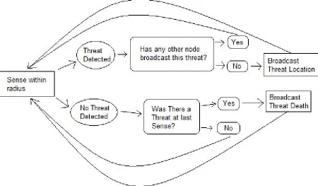
2.2 Wireless Sensor Node State Machine . . . 19
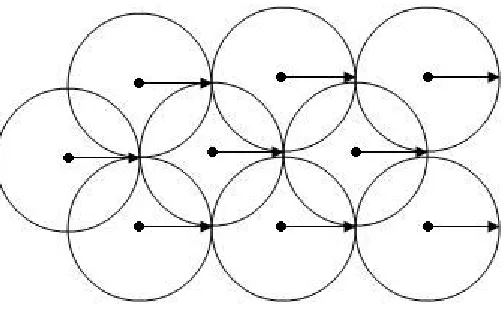
2.3 First Possible WSN Distribution . . . 20
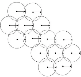
2.4 Second Possible wireless sensor node Distribution . . . 21
2.5 Simplified wireless sensor node Layout . . . 24
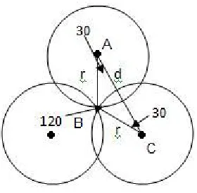
2.6 wireless sensor node Triangle . . . 24
2.7 Distance Triangle . . . 25
2.8 Y Offset Triangle . . . 25
2.9 Robot State Machine . . . 27
3.1 Simulation with 35 obstacles . . . 31
3.2 Simulation with Robots and Wireless Sensor Nodes . . . 32
3.3 Vary Repulsion Performance . . . 34
3.4 Small Repulsion Distance . . . 35
3.5 Large Repulsion Distance . . . 35
3.6 Vary Repulsion, Average Robot Lifetime . . . 36
3.7 Random Wireless Sensor Node Placement Performance . . . 39
3.8 Random Wireless Sensor Node Placement, Average Robot Lifetime . . . 40
3.9 Screen Shot of Random Wireless Sensor Node Placement . . . 41
3.10 Vary Number of Robots Performance . . . 42
3.11 Vary Number of Robots, Average Robot Lifetime . . . 43
3.12 Vary Threat Arrival Rate Performance . . . 45
3.13 Vary Threat Arrival Rate, Average Robot Lifetime . . . 45
3.14 Vary Number of Obstacles Performance . . . 47
Chapter 1
Introduction
In recent years, improvements in cooperation among robots and interest in academic and industrial fields have led to the use of cooperative robots to solve increasingly complex tasks. These include, but are not limited to, detection and containment, exploration, scouting, security, patrol, and public safety. The specific task that is the focus of this work, is that of surrounding and containing an object that is considered a “threat.” A future application that influences this concept is the idea of dropping the robots off in a remote location for an extended period of time. For this work, a practical application could consist of robots that are deployed in the sea off the coast of Alaska. The task of these robots is to surround and contain an oil spill, should an oil spill occur in the sea. Their job is not to clean up the oil, but rather to encircle the oil and contain it in that location until the arrival of those designated to perform clean-up procedures. However, the applications of this research are endless. The algorithms and concepts can be applied and modified for use in a variety of disciplines. The cooperative robot containment task involves a number of separate entities that must work together in order to solve a larger problem. This work is done in the “MAHESHDAS” simulator created solely for this purpose. The movements to be analyzed include how the robots react to mul-tiple threats, how the robots are attracted to threats, and how the robots are repelled by other robots, wireless sensor nodes, and other obstacles. Other issues include the use of wireless communication and the formation of teams, the definition of a “surrounded” threat, the introduction of wireless sen-sor nodes, the introduction of obstacles, different placements of wireless sensen-sor nodes, and how the robots perform when no threats are detected in the environment. The robots have multiple modes of operation that are analyzed to determine which is best under differing circumstances. Previous work has involved some of these aspects of cooperative robots. The same methods will be incorporated in this work. The algorithms have been modified slightly. The present work focuses on the addition of wireless sensor nodes, and how their use in the system improves the battery life of the robots. In order for this work to be validated, an accurate battery model is implemented. The present work reveals how the average life of the system changes under various conditions with the aid of wire-less sensor nodes. It also shows how the performance level is varies in comparison to simulations without the use of wireless sensor nodes.
The robots are simple, inexpensive entities. They contain no global knowledge and no central control. These robots use their limited knowledge to dynamically form teams to surround and contain one or more threats within the system. Since the end goal of the system is to quickly contain threats, the performance of the system is measured with respect to its ability to contain threats in a timely manner. Two measurements are recorded to determine the performance of the system. The percentage of threats contained and average threat containment time are tracked to discover advantages and disadvantages in a variety of situations.
A number of different techniques are use to provide a solution for the multi-threat containment problem. Cooperative robot techniques are used along with dynamic team formation, distributed control [17], and wireless communication. Cooperative robotics can be used in applications in-volving robots that work together to perform a set of tasks. These scenarios include the location and movement of objects, the playing of soccer games, and exploration of an environment. Wire-less communication has been used with varying technologies and applications including wireWire-less sensors, bluetooth headsets, wireless internet, radio frequency, microwave, and infrared. These approaches lend themselves well to solving the multi-threat containment problem.
1.1
Cooperative Robots
Cooperative robot solutions are centered around the idea that many inexpensive robots are better suited to solve certain problems than fewer, more expensive robots. For example, one large robot might work well in a automotive plant to weld door hinges on a car. Many cooperative robots might be better suited to play soccer, as soccer is inherently a team sport, and would require cooperation.
When creating a system that uses a number of cooperative robots, the system should be created in such a way that the loss of one or more robots would have little impact on the performance of the system. This is one major advantage of using multiple robots that work together as opposed to one larger, more expensive robot. The loss of one large robot would impede the ability to complete the task at hand. In a multi-robot system, the loss of one robot would have little to no impact on the performance of the system. An algorithm that reflects this behavior is called the ”swarm algorithm”. This algorithm was derived from observing insects line ants and bees that swarm to a threat. The loss of one ant or bee goes unnoticed when viewing the performance of the swarm algorithm from a high level. Likewise, the accomplishment of the insects’ goal is unaffected by the loss.
1.1.1 Robot Teams
Robot teams have been utilized in a number of ways to solve a variety of problems in recent years. Robot teams have been used in situations where human teams typically have been the best solu-tion. These areas include playing games and sports, hunting, cleaning, exploration, target tracking, and moving objects. One major advantage of utilizing robot teams, is that smaller, less expensive robots can be used and reconfigured to solve a variety of tasks. Robots built to solve a problem independently tend to be more expensive and are built specifically for that particular task.
groups, static and dynamic teams. Dynamic teams change over time, while static teams are defined at one point in time, and do not change.
1.1.2 Robot Formations
Robot Formations have been developed as long as cooperative robots and robot teams have been in existence. Research shows that a group of robots can be programmed to make a formation on their own. This has been accomplished in two ways. The centralized approach has one central authority which controls all of the robots. The other method is the distributed control method, where the robots make their own decisions. This work utilizes the distributed methodology, as it involves a large number of widespread robots. A centralized method would be too difficult to implement using multiple inexpensive robots, if at all possible.
The decision not to use a centralized method of robot formations for this work centers the fact that the robots modeled are small and inexpensive. If the robot in charge of delegating tasks were to die or fail, the entire system would fail. Conversely, a system with multiple robots, using a decentralized approach would see very little impact from the failure of one robot.
A variety of formations have been studied with respect to robot teams. Robots have been pro-grammed to form lines, triangles, and other multi-sided shapes. This work focuses on a circular formation, due to the circle’s uniformity. The threat is located in the center of the circle, and the robots form the circle with the knowledge that their distance from the threat is the radius of the circle. To be more specific, the robots do not really form a circle as humans define a circle. Techni-cally, the robots form a multi-sided polygon. If eight robots were to form a “circle” around a threat, they would actually be forming an octagon. Likewise, five robots would form a pentagon. The exact shape is defined by the number of robots involved in its formation.
1.1.3 Swarm Intelligence
Swarm intelligence is a field of research which involves the implementation of multiple robots. This model of distributed systems was developed in the image of birds, bees, ants, and schools of fish. An important advancement developed in swarm intelligence is the ‘social’ component. This component is made possible through sensors, and in some cases, wireless communication. Each node makes observations of it’s surroundings, and makes a decision on how to act based on previous decisions and feedback from other nodes.
While using this ‘social’ component, the number of neighbors is usually limited by the ability of sensors on the node. The sensors allow the nodes to react to a dynamic environment, but they limit the individual’s knowledge of the complete system. This spatial limitation is one of the major challenges presented in swarm algorithms. The individual nodes are limited by their sensing range. However, this can be overcome through the use of multiple nodes. While an individual node may not be aware of the activities in a more distant section of the environment, there are most likely other nodes in that section able to perform the same task.
Jones et al. use a potential field based approach to attract the robots toward threats and away from other robots.
Nodes in a swarm intelligence environment can also utilize wireless communication to access a larger area of perception of the environment. Different networks can be set up to transmit informa-tion. However, adding more advanced wireless communication makes the system and nodes more expensive. This becomes counter productive, as the advantage of utilizing swarm intelligence, is that each individual node is inexpensive and simple. However, the addition of wireless communication is still possible in swarm algorithms.
While one node may not be able to perform the task at hand by itself, the combination of multiple nodes creates a system that is very efficient at performing certain tasks.
1.1.4 Robots with Static Sensor Nodes
Robots working cooperatively with static nodes is a new research area in the cooperative robot field. While Krogh et al. investigated basic communication between robots and static nodes in [3], Seow et al. investigated more complex communication in [4]. The purpose of [4] was to use static sensor nodes to aid robots in localization.
The static nodes know their location in the environment, and the mobile robots can determine their own global location by tracking their own movements and listening to the static nodes’ loca-tion. A particle filter is used to determine the location in this dynamic environment. This research also proves beneficial in the robot’s ability to formulate an accurate knowledge of its global location.
1.2
Wireless Communication
Due to the fact that this work incorporates wireless sensor nodes, it is important to understand wireless sensor networks. The difference between the two, is that the nodes, are just that, individual nodes. A wireless sensor network is comprised of multiple wireless sensor nodes, working together. Wireless communication has been incorporated in a wide variety of fields including computing, sensing, cellular phones, radios, and remote control. The technology has progressed to include radio frequency, wireless LAN, and bluetooth applications. Ransom improved the modified MAHESH-DAS simulator in [24] to include wireless communication between nodes. He utilized Frequency Division Multiple Access (FDMA) approach to allow for multiple channels of communication.
The addition of wireless communication to the MAHESHDAS environment gave the nodes the advantages of (1) detecting threats outside the node’s sensing range, (2) limiting the number of robots attempting to surround a threat, and (3) establishing the loyalty of each robot.
state, the node must ensure that that power saved by sleeping for the determined amount of time, will save more energy than will be lost by switching states to sleep and back again.
With the multiple applications feasible for wireless sensor nodes, each network may have differ-ent performance requiremdiffer-ents. Therefore, a differdiffer-ent networking protocol may be used. Some dif-ferent protocols are analyzed in [16]. One of the first protocols used with wireless sensor nodes was flooding, which is used as a benchmark for most new protocols. However, flooding has deficiencies, therefore new protocols have been developed. Gossiping is one branch of flooding. A data-centric protocol, SPIN (Sensor Protocols for Information via Negotiation), is another early development using ADV, REQ, and DATA messages. LEACH (Low Energy Adaptive Clustering Hierarchy) is a cluster-based protocol which randomly rotates cluster heads to evenly distribute work load. Finally, a geographic protocol, GEAR (Geographic and Energy Aware Routing), uses the location of the nodes to route the packets in order to reduce data transmission costs. Dai et al. concluded that it is not possible to design a routing protocol which has acceptable performance levels for all scenarios under all applications. Each protocol is efficient for different characteristics of each application. As a result, different desired characteristics require the use of different protocols.
At another level, research exists on wireless sensor node architecture as noted in [28]. This research was done on LMNP, which was developed in 1992. This centralized architecture was appropriate for a LAN, but did not scale well. Subsequently, SNMP was developed for this scaling reason, since SNMP uses polling, this makes it unsuitable for wireless networks. Duan and Yuan preferred ANMP for mobile wireless ad hoc networks. It saves energy, has a distributed hierarchal architecture, and is self-adaptive. Duan and Yuan then proposed a task-oriented clustering algorithm based on ANMP. This provides scalability, task orientation, and is lightweight. For their simulations, the nodes were placed randomly on a 150 x 150 meter grid, and each node had a sensing range of 10 meters. The two scenarios used were a cluster forming scenario and a data collecting scenario. This new architecture was successful in saving energy for the entire sensor network.
A system similar to the proposed system in this paper is found in [3]. Here, the nodes are divided into sentry nodes, and non-sentry nodes. The sentry nodes perform constant basic sensing and communication. Meanwhile, the non-sentry nodes sleep for a designated period of time, then switch to full power only when needed to provide more refined sensing for tracking. Similar to the proposed work, the sentry-based system allows the non-sentry nodes to conserve battery power when they are not needed. Here, the sentry nodes would be equivalent to wireless sensor nodes, and the non-sentry nodes would be similar to the robots. In [3], the sentry nodes explicitly tell the non-sentry nodes when to switch to full power. This reduces the risk of some non-sentry nodes will be in different states than other non-sentry nodes. However, this is a step toward a more centralized network.
Ants deposit pheromone on their way to a destination. As more ants take a certain path to the destination, the concentration of the pheromone increases for the shortest paths. Future ants travel on the paths that have the highest concentration of pheromone, which tend to be the shortest paths. Probability algorithms are developed in [26] that allow the Ad Hoc network to find new shortest paths in a mobile wireless network. This paper investigates just a few available routing protocols that can be used in wireless networks, and proposes a new protocol intended for use in mobile wireless networks.
1.3
Battery Modeling
Further work exhibits a better understanding of the characteristics of batteries. When new electronic devices are developed, it is important to have an accurate estimate of the expected battery life of the product. A cost effective means of calculating this, is through battery modeling. An estimate can then be made without the time and money required to develop a prototype.
Tests performed on common batteries reveal characteristics of the batteries. This data can be programmed into a simulator along with the power requirements of the device. Using mathematical equations that vary in complexity, one can determine the expected lifetime of the batteries used in the device.
A variety of battery models calculate the exact terminal voltage based on internal battery char-acteristics and current rate. For the purposes of this experiment, the terminal voltage is assumed to be ideal. Nine volts will be supplied to the nodes. One area of concern lies with the extent of bat-tery life. Therefore, the batbat-tery models proposed are those that focus on remaining batbat-tery capacity. Other areas of interest include models that focus on embedded systems, robots, or mobile platforms.
1.3.1 Common Battery Models
Most battery models require data related to current, time, voltage, and capacity. Other models require knowledge of the frequency of draining current to model capacitive battery properties. A variety of models measuring the performance of batteries operating with a constant drain on the battery are compared in [29] and [18]. Other models are used to describe battery capacity in a system such as those found in [20], [21], [27], [8], and [22].
Battery models found in [29] provide a choice between varying accuracies and complexities. The first model called the Ideal Model, ignores the internal parameters of the battery. In this model, the battery is represented as a simple voltage source. The next model, the Linear Model, considers the internal resistance of the battery. The voltage and internal resistance for the linear model are solved using equations 1.1 and 1.2.
E =E0−k·f (1.1)
where
E0 no load voltage when fully charged;
f state of discharge;
R0 internal resistance when fully charged;
k, KR constants obtained by experiments.
The final model proposed in [29] is the Thevenin Model. This model expands upon the linear model to include overvoltage, which is represented using a parallel combination of a capacitor and resistor in series with the resistor representing the internal resistance of the battery. The Thevenin Model is more accurate than the Linear Model, but Kim et al. clearly state that obtaining exact values mathematically using the Thevenin Model is “very difficult and time consuming.” Kim et al. use a SPICE program to perform battery simulations.
Further battery modeling information is gained from [20]. Here, it is discovered that the end of a battery’s life is determined when the cell capacity falls below 80% of its original value. Medora et al. also describe how the internal resistance of the battery increases with diminishing battery capacity. When the battery reaches 25% of charge, the internal resistance increases rapidly.
Peukert’s Law is a prevalent term among battery modeling literature. This is found in [20], [21], [23], [18], and [14]. This law states that the battery’s capacity decreases as the discharge rate increases. In other words, as the current being drawn from the battery increases, the total available power of the battery decreases. This occurs because, at large current drain, some current is lost. Equation 1.3 reveals how a larger current load decreases the total stored capacity. While the component receives a current ofI, the battery loses a current ofIk.
Cp =Ik·t (1.3)
where
Cp capacity according to Peukert, at a one-ampere discharge rate; I discharge current;
k Peukert constant(typically 1.1-1.3);
t time of discharge.
such as [27], [25], [14], and [8] require extremely complex models to simulate recovery effect. Specifically, [22] states, “relative to the recovery effect, the rate capacity effect influences more critically battery capacity. For this reason, we will consider only the rate capacity effect in our model.” Essentially, the additional complexity required to model the recovery effect outweighs any improved accuracy gained.
1.3.2 Modeling Batteries in Wireless Networks
While modeling batteries is not uncommon, modeling batteries in a wireless network is a new research area. Jayashree et al. modeled batteries in an AD HOC wireless network to develop a protocol that is best suited to conserve battery power [25]. Jayashree et al. developed a complex Markov chain to model rate and recovery capacity effects. Here, the theoretical capacity of the battery is differentiated from the actual battery capacity. The actual battery capacity can never be greater than the theoretical battery capacity, because power can be lost through rate capacity effect, but never gained above the original theoretical capacity through recovery capacity effect.
The model used in [25] divides time into slots. If current is being drawn from the battery, the battery loses capacity according to the current drain and rate capacity effect. If no current is being drawn from the battery during a period of time, then the battery’s capacity is replenished according to the recovery capacity effect.
As mentioned earlier, the rate capacity effect will be modeled in this work. The additional complexity introduced from modeling recovery effect outweighs the minute increase in accuracy that recovery effect provides. Therefore, recovery effect will not be modeled in this research.
1.3.3 Energy Conservation in Processors
In immobile computing systems, the processor is the main source of energy consumption. Kadayif et al. investigate an energy saving strategy based on adaptive loop parallelization in [11]. This strategy puts some processors in sleep states when they are not needed. This is determined at compilation time to reduce the performance impact at run time. There is a performance impact because there is overhead involved in computing when processors should enter or leave various sleep states. Kadayif et al. also introduce a prediction strategy, so the processors can predict when to leave the sleep state before they are actually needed. This also helps to reduce the performance impact by entering the sleep state. If the processor leaves the sleep state too soon, it wastes more energy by being in an active state longer. If the processor leaves the sleep state too late, there is a performance cost while the processor is leaving the sleep state.
Chapter 2
Methodology
As the MAHESHDAS simulator is capable of more advanced algorithms, it is important to con-sider real-world applications. In creating this system in actual hardware, it becomes apparent that the expected lifetime of the robots is extremely short. It would be inefficient to spend the time implementing this system without a means to extend the lives of the robots.
With this in mind, wireless sensor nodes can be added to the system. They would constantly sense for threats, allowing the robots the ability to sleep no threats are detected in the system. This lack of motor use conserves battery power and extends the robots’ lives.
Another step toward more realistic modeling is to make the robots avoid the wireless sensor nodes. If the wireless sensor nodes are in the environment providing aid via sensing and wireless communication, they should be avoided by the robots. Furthermore, obstacles can be placed in the system to represent any object that may exist in a real world environment. That allows the robots to avoid them as well.
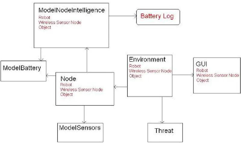
A graphic example of the major MAHESHDAS components can be seen in Figure 2.1. The major changes for this work are highlighted in red. The Environment class is the central structure where the simulation environment is built. All of the nodes are placed and tracked in the Envi-ronment. The Environment also keeps track of which node will perform the next action. As the wireless sensor nodes and obstacles were added to the simulator, the Environment class changed to accommodate them.
The Environment contains nodes and threats. The Threat class was left unchanged. The Node class and ModelNodeIntelligence class had the most changes. Instead of a node just representing a robot, a node now has to accommodate wireless sensor nodes and obstacles. Every action and characteristic of the Node class had to be redefined as it pertains to robots, wireless sensor nodes, and obstacles.
The ModelBattery class had changes to update how the battery drains power according to the battery model that has been developed. It was also updated to use exact current drain and time of drain according to common components.
The battery log is a text document that was added to keep a record of each node’s remaining battery capacity throughout the simulation.
The GUI was also updated to receive commands for wireless sensor nodes and obstacles. It also draws those nodes differently on the grid.
an efficient means of getting full coverage of the environment while using a minimal number of wireless sensor nodes. There may be cases where absolute control of the location of each wireless sensor node is impossible, and for this reason a random wireless sensor node placement scheme is also investigated.
With these additions, an accurate battery model is necessary to understand any changes in bat-tery life that occur as a result. The primary goal of this work is to extend the average lifetime of the robots through preservation of battery life.
2.1
Battery Model
In order to get an accurate lifetime expectancy of the robots, it is important to be able to model the battery which powers these robots. There are a number of models available to achieve this goal.
The predicted battery power should be accurate, but it is not imperative that it predict the battery life to the nearest second. Since every simulation will be subject to the same battery model, any discrepancies will be automatically included in every simulation. The simulations will be compared amongst each other to determine any degradation or improvement in average battery lifetime.
2.1.1 Values Derived
For this work, the battery model utilized is slightly more accurate than the linear model. The linear model offers simplicity in calculations. However, the addition of Peukert’s Law and “rate capacity effect” result in a more accurate model. Peukert’s Law and rate capacity effect have little effect on small current values, like those found in wireless communication. On the other hand, more current is wasted when the motors are running, due to their larger immediate current drain. The battery model used in this research ignores phenomenons such as “recovery effect”. Tracking this information would require more calculations and would add more complexity. The addition of Peukert’s Law and rate capacity effect to the linear model is sufficient enough to reveal trends in the robot lifetime of the robots.
In order to put this realistic battery model to work, components that would be found in the real robots should be used to determine values such as voltage, current drain, wireless current character-istics, sensing time, and sensing distance. These values can be seen in Table 2.1 and were derived from [5], [7], [6],and [12].
Battery values for robots were derived from common, rechargeable battery packs. The battery values for the wireless sensor nodes were derived from Energizer 9V battery values [10]. The wireless sensor nodes use the smaller 9V batteries instead of the larger 9V battery packs as the 9V batteries are smaller and less expensive. They provide sufficient capacity such that the wireless sensor nodes battery life in never a concern during simulations. The robots routinely die prior to the wireless sensor nodes.
for sensing time came from the sonar sensor. All current drains were combined to produce the final current drain values.
Likewise, the wireless nodes were modeled from common wireless devices currently available. These sensors have slightly different values for transmission and receptive values. The data being sent over the wireless nodes is sent using very small data packages. These transmissions need only a small amount of data in order to communicate all of the information needed in these simulations.
Parameter Value
Battery Voltage 9V
Robot Battery Capacity 1600 mA*h Wireless Sensor Node Battery Capacity 600 mA*h
Motor Current Drain 960 mA Robot Sensor Current Drain 60 mA*h Wireless Sensor Node Sensor Current Drain 30 mA*h Wireless Transmission Current Drain 22 mA
Wireless Receive Current Drain 27.7 mA
Motor Move time Varies
Node Sense Time 20 ms
Wireless Transmission Time 4 ms Wireless Receive Time 4 ms
Sensing Distance 1 m
Table 2.1: Simulation Battery Values
2.1.2 Information Contained in Battery Log
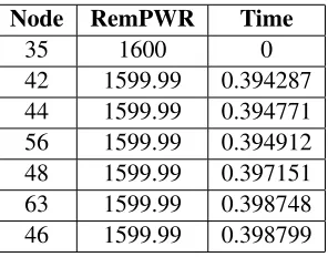
A battery log was developed to track the remaining battery capacity of each node. When a node uses current to perform a task (ie. move, sense, or communicate), the battery log records the nodes ID, the current simulation time, and the remaining battery capacity of the node. This data is useful later in the experiment. An example of this battery log can be seen in table 2.2. It should be noted that the time kept in the battery log is in units of seconds. The time displayed on the plots shown later is in units of minutes, because it is easier to comprehend units of minutes at a larger scale.
2.1.3 Organization of Data in Battery Log
When the battery information is entered into the battery log, it is not in it’s original state. There needs to be appropriate formatting performed on the data in order to make it more descriptive of each node, and the system as a whole.
Node RemPWR Time
35 1600 0
[image:25.612.237.385.100.216.2]42 1599.99 0.394287 44 1599.99 0.394771 56 1599.99 0.394912 48 1599.99 0.397151 63 1599.99 0.398748 46 1599.99 0.398799
Table 2.2: Initial Battery Log
in the battery log. For this reason, the first modification to the battery log, is to remove redundant entries. Other than removing redundant entries, the formatting remains consistent to that seen in 2.2.
Upon removal of the redundant entries, the values are parsed into individual files for each node as seen in table 2.3. This provides each node with its own storage file. However, these files are extremely large. A chart containing 1000 data points is cluttered and difficult to interpret. A chart with 100 data points reveals the same information in a more concise manner.
RemPWR Time
1600 0
1600 0.099514 1600 0.199514 1599.99 0.199514 1599.99 0.299514 1599.69 0.399514 1599.31 0.499514
Table 2.3: Individual Node Battery Log
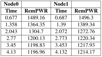
In order to reduce the data to a more manageable size, one can specify the magnitude that will accomplish this reduction, or thinning of data. An example of one robot’s thinned file can be seen in table .2.4. In addition, a file is created with all of the nodes’ data thinned out as seen in table 2.5. This is only a small section of the table. In reality, there would be two columns for each node. This file can easily be copied and pasted into Microsoft Excel in order to plot the data. Furthermore, the thinning also creates a file with the time of death of each node. This valuable data helps determine the average death for the nodes in the simulation and the standard deviation of the time of death.
[image:25.612.252.368.391.508.2]RemPWR Time 1493.86 45.8986 1360.45 91.7986 1345.44 132.899 1271.65 177.299 1194.68 220.399 1193.00 261.099 1190.76 301.799
Table 2.4: Thinned Node Battery Log
Node0 Node1
Time RemPWR Time RemPWR 0.677 1489.16 0.687 1496.3 1.358 1364.35 1.39 1389.34 2.043 1304.7 2.072 1272.76 2.77 1200.13 2.773 1220.34 3.45 1198.83 3.453 1217.93 4.13 1196.96 4.132 1214.17
[image:26.612.207.413.483.599.2]and clear. The data revealed through the battery model and log can be clearly understood to reflect the behavior of real nodes, and the data can be considered accurate enough to reveal the trends seen by modifying different variables.
2.1.4 Battery Model Used
Modeling the battery life of the robots and sensor nodes is important in gaining a general under-standing of the expected battery life of the components. It is important to be as accurate as possible without over complicating the already intricate system. The purpose of the battery modeling is to help prove that the addition of wireless sensor nodes, and the modification of the robots’ algorithm will allow the robots to operate longer on the same battery. Therefore, the battery model must be able to reveal any changes in the life of the batteries.
A number of battery models have been considered, and the optimal battery model to begin this task is the linear battery model seen in equation 2.1. It does the job of taking away power from the batteries without getting into impacts from frequencies, varying currents, or capacities.
Cap(mAh)=P revCap−I(mA)·T(h) (2.1)
An improvement can be made to this equation to account for various battery properties without adding much overhead to the system. The equation from 1.3 can be added to equation 2.1. This results in equation 2.2
Cp=Ik·tCap(mAh)=P revCap−Ik·t (2.2)
According to [23] the value ofkis more accurately, 1.28 at room temperature. This equation is sufficient for modeling battery life with respect to current being drained over time. Research has included other characteristics such as recovery effect. In some cases recovery effect was ignored as it was shown that rate capacity effect had a larger impact on battery capacity, and was easier to implement. The research that did implement recovery effect did so through designing a complex model solely committed to battery modeling. This was mostly done using powerful software such a Pspice. Since the MAHESHDAS simulator is written in C++ and JAVA, it would be difficult and time consuming to convert this previous work to C++. This work focuses on improvements made by the addition of wireless sensor nodes to the system, making it unnecessary for added complexity at this point. The battery modeling needs to be accurate enough to reveal the manner in which wireless sensor nodes in the system allow the robots to conserve battery power. Considering the current drain and the amount of time during which this occurs, it is important to obtain an accurate model of battery capacity. This accuracy can be further improved by considering Peukert’s law and rate capacity effect. When large currents are drawn from the battery, the total available energy in the battery decreases due to lost current.
simplify experiments, the battery capacity will begin at 1600 rather than 2000 milli ampere hours. The battery is then considered dead when it falls below zero.
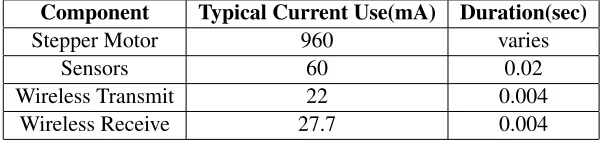
Based on common components employed in robotics today, typical currents and amount of time utilized were found in [5], [7], [6], and [12]. With all of the peripherals in place, it is assumed that processor power is negligible at this point. Both models would use the same processor power, thereby negating the need to model the processor power.
Component Typical Current Use(mA) Duration(sec)
Stepper Motor 960 varies
Sensors 60 0.02
Wireless Transmit 22 0.004
[image:28.612.159.462.202.274.2]Wireless Receive 27.7 0.004
Table 2.6: Power Consumption of Components
The numbers in Table 2.6 are derived through building a virtual robot. The motor value is derived from [5]. The stepper motor 39BYG was chosen which operates at 9V. It consumes a 0.48A or 480mA. This robot would use two stepper motors to control two wheels, thereby using twice as much current, making it drain 960mA. The amount of time during which the motors turn is dependent on the distance the robot is traveling. This robot might also use sonar and/or IR sensors, possibly along with a CMUCAM2 for color detection. Information can be taken from [6] and [12] to determine that each device uses roughly 30mA, thereby a noting that a combination of two of these sensors would drain 60mA. The sonar sensor takes about 0.02 seconds to obtain a distance reading. The IR sensor works instantaneously, therefore the sonar sensor is used for the timing of the sensors. Finally, using [7], MICAz wireless motes would use 22mA to transmit data and 27.7mA to receive data. Assuming the amount of data sent is approximately 1kB, it takes 0.004 seconds to transmit the data. The data size of 1kB is chosen because this is the largest size that would be needed to communicate locations and wether the threat is alive or dead. These are the data values that will be employed in simulations.
Essentially, the robots have two different modes of operation; sleeping, and moving. When modeling the battery power consumed during these two modes, it is sufficient to continue recording the power used by the peripherals. During the simulation, the battery power used by the processor is negligible, because it uses considerably less power than is used by the peripherals, and the processor is constantly active regardless of the movement state of the robots.
energy saved by entering the sleep mode for the predicted amount of time will be worth the cost of transitioning between sleep modes. The robots are free to sleep when there are no threats in the environment, and then begin moving again once a threat is detected.
2.2
Wireless Sensor Nodes
The major addition to this project is the use of wireless sensor nodes. These are introduced to the system for the purpose of helping to conserve the battery life of the robots.
2.2.1 The Wireless Sensor Nodes
The wireless sensor nodes are essentially robots that remain stationary. They have the same sensing capabilities and wireless communication as robots. The wireless sensor nodes begin with a different battery capacity from the robots because the wireless sensor nodes run on 9V batteries, as opposed to 9V battery packs. Using a 9V battery is less expensive than using a 9V battery pack. Since the wireless sensor nodes draw less current that robots do, the wireless sensor nodes can use the 9V battery, that has a small capacity than the 9V battery pack. The life expectancy of the wireless sensor nodes is greatly enhanced by its lack of movement. Therefore, using a smaller battery is not detrimental to the wireless sensor node’s life expectancy. The wireless sensor nodes conserve a significant amount of power by remaining stationary because motors drain more current than any other component.
2.2.2 Algorithm Modifications
In order for the addition of the wireless sensor nodes to affect the robots, modifications needed to be introduced into the existing algorithm. Changes made directly to the robots will be explained as well as any changes resulting from the wireless sensor node’s role.
The purpose of adding the wireless sensor nodes is to conserve the battery life of the robots. The major battery draining component on the robots is the motor. To ensure that the robots remain stationary until needed, they are designed not to move until a threat is introduced into the system. The robots and wireless sensor nodes monitor the number of threats in the system via wireless com-munication. When there are no threats present, the robots cease moving and sensing. They will return to those actions when they receive a wireless signal from a wireless sensor node communi-cating the appearance of a threat. The robots then continue their algorithm as usual for locommuni-cating and containing threats.
Figure 2.3: First Possible WSN Distribution
Since the wireless sensor node is a part of the Node class, it can utilize the same wireless communication as the robot. The wireless sensor nodes do not listen to any broadcasts. They just transmit whatever they sense for the robots to receive.
For optimal efficiency,the wireless sensor nodes need to be placed in the system strategically. Thus, they should not be placed randomly in the simulation. When there are no threats present, the wireless sensor nodes are the only source for sensing threats. Since they can not move, they must be able to cover the entire grid without allowing any threats to go undetected. Utilizing the sensing radius of the wireless sensor nodes allows one to disperse the nodes in a way that overlaps the wireless sensor nodes’ sensing areas, and requires the minimum number of wireless sensor nodes. Two possible options for distributing the wireless sensor nodes can be seen in 2.3, and 2.4. The arrows in the figures represent the sensing radius of the nodes. The placement seen in 2.4 is the most efficient, so this layout is used in the MAHESHDAS simulator, and is tested against random wireless sensor node placement.
Random placement is where each wireless sensor node’s location is determined randomly. With random wireless sensor node placement, the possibility exists, that a threat could appear on the grid in a location and go undetected by any wireless sensor node. For this reason, robots move constantly while using random placement of wireless sensor nodes. Here, the purpose of the wireless sensor nodes is to sense the majority of the threats and provide the robots the location of those threats immediately, without the need for the robots to get close enough to the threats to sense them with their limited range sensors. However, this random wireless sensor node placement inherently limits the lifetime of the robots.
Since the wireless sensor nodes remain stationary, they can not participate in the actual contain-ment of threats, and therefore can not be considered a valid threat containing system component.
occupy the larger amount of space required by the robots. Therefore, the wireless sensor nodes do not have a large impact on the robot movement algorithm. The robots have more room in which to maneuver around the smaller wireless sensor nodes compared to the size of other robots.
The robot repulsion from wireless sensor nodes is slightly different from robot repulsion from other robots. When robots attempt to avoid other robots, they must predict the worst case scenario, that the other robot is moving directly toward the first robot’s desired path. Since the robots know that the wireless sensor nodes do not move, additional calculations are not required to predict the worst case movement of the wireless sensor nodes. Furthermore, the wireless sensor nodes have a smaller radius that the robots, so the robots can move around them easier.
2.3
Obstacles
In order to make the simulator more realistic, more modifications are required. Since, typical ground is not perfectly level and foreign objects could exist within the field, random obstacles are added to the simulation environment to represent such circumstances.
2.3.1 The Obstacles
The simulator obstacles are simple and round, with a variable radius, that can be changed as desired. The obstacles do not affect the sensing ability of the wireless sensor nodes or robots to detect threats or other nodes. They serve only as an additional obstacles for the robots to avoid.
2.3.2 Algorithm Modifications
The addition of obstacles does not significantly impact the robot’s algorithm. The obstacles are stationary nodes that do not sense or use wireless communication. They do not contribute to the detection or containment of the threats. They are simply obstacles to be avoided as the robots work to contain the threats.
2.4
Random Wireless Sensor Node Placement
As previously mentioned, developing a uniform placement for the wireless sensor nodes is ideal. However, some environments are not ideal for uniform wireless sensor node placement. These may contain variations in elevation, imperfect sensing radii, obstacles, and inaccessible terrain. When this occurs, it is important to investigate a random wireless sensor node distribution. This models a case where wireless sensor nodes are placed in the environment randomly, without following a defined distribution. This type of distribution might occur if wireless sensor nodes were dropped into the environment via an air vehicle if the location where the wireless sensor nodes are to be distributed is too remote or dangerous for human beings to access on foot.
this may leave gaps in the sensing area. Other places in the environment may be be too cluttered with too many wireless sensor nodes.
To alleviate the issue of gaps in the coverage area, simulations run with a random distribution do not allow the robots to sleep. Even when there are no threats in the system, the robots continue moving as if there were no wireless sensor nodes present in the system, which in turn, creates a continuous drain on the robots’ battery power. The purpose of wireless sensor nodes in this case, is to extend the searching area of the robots. Without the wireless sensor nodes, the robots can only sense within their own limited sensing range. With the wireless sensor nodes in the system, the sensing area of the robots is extended. The wireless sensor nodes continue to have the ability to broadcast the approximate location of a sensed threat, thereby informing the robots of the location of that threat. The robots then proceed toward the threat, and can now do so when a threat exists beyond a robot’s individual sensing range.
A scenario containing a random placement of wireless sensor nodes with robots that sleep when no threats are present in the system, is an option. However, there is the potential for threats to appear in the system, and without being sensed if the wireless sensor nodes are located such that the threats are beyond the sensing range of each of the wireless sensor nodes. While this would preserve battery life, it would also decrease performance. In order to justify the methods used in this research to conserve battery power, the performance must be at or above the performance of the robots when wireless sensor nodes are not present in the system.
2.5
Uniform Wireless Sensor Node Placement
As mentioned earlier, whenever possible, the wireless sensor nodes should be placed in the system in a uniform manner. The distribution with the most overlap can be see in Figure 2.3. This would be advantageous if the wireless sensor nodes were prone to early deaths or malfunctions. Since this is not an issue, the more efficient layout is used, which can be seen in Figure 2.4. Here, there is less overlap, but fewer wireless sensor nodes are required. This saves money and poses fewer obstacles for the robots to avoid.
With the advantages inherent in the layout in Figure 2.4, it is the chosen layout for simulations in this research. Using this hexagonal distribution, there is a mathematical way to calculate where the wireless sensor nodes should be placed in relation to each other.
Figure 2.5 reveals the angles at which the wireless sensor nodes are placed in relation to each other. The circles in the drawings represent the sensing range of the nodes, with the center of each circle representing the location of the nodes. There is one central node in the layout, with six nodes spaced evenly around it. Six nodes spaced even over 360 degrees, means that there must be 60 degrees between the location of each outer node.
Figure 2.5: Simplified wireless sensor node Layout
Figure 2.7: Distance Triangle
Figure 2.8: Y Offset Triangle
The triangle in Figure 2.6 can be simplified into a right triangle by dividing it in two, between the midpoint of leg ‘d’ and the 120 degree vertex. The resulting Figure 2.7, is used to calculate ‘d.’
With the sensing radius known, the distance between nodes can be calculated using equation 2.3, where r is the sensing radius.
d= 2r·COS(30) (2.3)
Applying this to Figure 2.5, the distance between nodes can be used as the offset of the x-coordinates between wireless sensor nodes with the same y-x-coordinates.
The offset in the x-direction is only half of the information needed to complete the layout. Figure 2.8 can be drawn to calculate the y-offset between nodes as well. The triangle drawn in Figure 2.8 leads to equation 2.4, where d is the distance between nodes that was calculated in equation 2.3. This value becomes the y-offset between rows. The next row will have a y-value of a difference of the y-offset. This row will be shifted by half of the x-distance between nodes, so each node falls between the nodes of the neighboring rows.
yOf f =d·SIN(60) (2.4)
complete coverage of the environment with minimal overlapping and the least number of wireless sensor nodes necessary.
2.5.1 Robots Sleeping
When there is a uniform distribution of wireless sensor nodes in the environment, such that the entire environment is covered by the sensing areas of the wireless sensor nodes, there is a guarantee that every threat will be sensed by a wireless sensor node. This complete coverage means the robots are not needed to sense the arrival of a threat. This can be accomplished by the wireless sensor nodes.
With the wireless sensor nodes constantly updating the robots with the status of the threats in the system, the robots can determine whether they are needed or not. Each robot receives wireless transmissions from the wireless sensor nodes when a threat arrives or disappears, allowing the robots to monitor the number of live threats in the system.
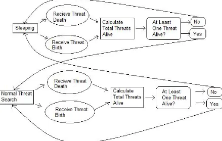
If there is at least one threat alive in the system, the robots should follow their usual random search algorithm previously developed. If there are no threats alive in the system, the robots should sleep. This allows the robots to conserve their battery power as their motors are not in use. Robots however, continue listening through the wireless receiver in the event that a wireless sensor node detects a threat.
When a robot receives a transmission that a threat has arrived, the robot resumes its search for threats using its onboard sensors. Figure 2.9 can be used to understand how the robot decides when it should move. In the sleep state, the robot does not move or sense at all. All it does, is listen for wireless communication. When the robot is in the normal threat containment state, it moves around the environment like it normally would in an environment without wireless sensor nodes. The robots search for threats to contain, form teams, and communicate amongst each other. The robots also listen for broadcasts from the wireless sensor nodes. If a wireless sensor node reports the death of the last threat in the environment, the robots know to change to the sleep state.
This is the manner in which robots’ battery lives are conserved. Table 2.1 reveals that the motors drain the most current. Therefore, if the robots shut the motors off when they are not needed, then battery life would be extended.
2.6
Wireless Sensor Nodes Broadcast Location
When Ransom added the ability for wireless communication, he also added the ability for the robots to call for assistance. When a robot senses a threat, it can broadcast its approximate location. Other robots receive this wireless transmission, which allows them to calculate the approximate location of the threat and move toward that location.
already operational, the wireless sensor nodes utilize this ability to call for help. This provides the approximate location of the threat to the robots.
Chapter 3
Results and Discussion
Simulations were run using the modified MAHESHDAS simulator. This environment was devel-oped to test the multi-threat containment scenario. MAHESHDAS provides a powerful event driven environment to model robot behavior in the threat containment problem.
The MAHESHDAS simulator consists of two parts. The front end is written in JAVA, and is used to display the Graphical User Interface (GUI). The second part, is the engine behind the simulator which drives all of the calculations. This part of the simulator, written in C++, tells the GUI what to display. The simulator can also be run without the GUI. The GUI provides a valuable tool to visualize the behaviors of the simulation that otherwise are not noticeable by simply looking at the data generated.
In some cases, unexpected behavior is observed in the results. When this happens, the GUI is useful to better reveal how the robots move within the environment. Screen shots of the GUI are also used to explain why some variations are observed in the results.
Simulations were run to test what impact that the addition of wireless sensor nodes has on the performance of the system and the average battery life of the robots. Performance is measured by both the percent of threats contained and the average containment time of the threats. Since the life span of a threat is 60 seconds, any threats not contained counted as 60 seconds toward the average containment time. This is necessary in order to obtain a performance penalty for a failure to contain a threat. There is no way to determine when the threat would have been contained, had it remained indefinitely. However, this does lead to a more accurate performance metric, as a failure to contain a threat should be detrimental to the performance metric.
3.1
Simulation Setup
Monte Carlo simulations are run using a modified MAHESHDAS simulator to test the proposed scenarios. These tests focus on the ability to increase the robot’s average lifetime while retaining similar performance. To fully understand the advantages and drawbacks of utilizing wireless sensor nodes, different parameters have been varied.
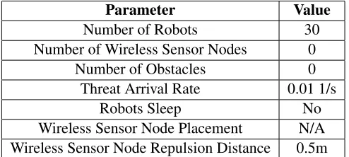
Table 3.1 shows the default parameters for each simulation. All low level parameters were derived from Ransom’s previous work, and verified to be realistic values. Unless otherwise specified, these are the values of each simulation. Each simulation was run for a time of 500 seconds. The same simulation would be rerun and results taken until at least 100 total recorded threats had entered the system and died. This insures that the impact of any one simulation giving unrealistic results is minimized.
Parameter Value
Number of Robots 30
Number of Wireless Sensor Nodes 0
Number of Obstacles 0
Threat Arrival Rate 0.01 1/s
Robots Sleep No
Wireless Sensor Node Placement N/A Wireless Sensor Node Repulsion Distance 0.5m
Table 3.1: Simulation Default Parameters Without Wireless Sensor Nodes
3.1.1 Obstacles
Obstacles have been added to the MAHESHDAS simulator to assist in creating a more realistic environment. These obstacles are simple components. They are considered to be nodes as defined by the previous MAHESHDAS environment thereby allowing the robots to be able to sense them as part of the obstacle avoidance algorithm. The Node class already provides a means of placing a round object within the environment. As a result, the Obstacles are shown as circles with a fixed radius of 0.2 meters. The locations of the obstacles can be specified using a text document. The obstacles do not move, sense, or communicate in any way.
Figure 3.1 shows a simulation with 35 obstacles placed randomly. For all of the screen shots with wireless sensor nodes, the wireless sensor nodes are four times their normal size so they can bee seen clearly. As the image reveals, the obstacles take up a large amount of space. This forces the robots to maneuver around a solid obstacle as opposed to a point, which is virtually what avoiding a wireless sensor node equates to.
3.1.2 Wireless Sensor Nodes
The wireless sensor nodes are also included as a part of the Node class. This is done for the same reason that obstacles are part of the node class. Similar to obstacles, wireless sensor nodes do not move either. They sense for threats and transmit data via the wireless communication already in place. In these simulations, the wireless sensor node’s radius is 0.01 meters.
threats.
3.1.3 Robots
The robots are virtually unchanged from the Node that was defined in the previous MAHESHDAS simulator. The major difference is that the robots now have the ability to sense for and avoid both wireless sensor nodes and obstacles. The robots can also receive wireless communication from the wireless sensor nodes, and use this information to decide if they should be moving, sleeping. Each robot monitors the number of threats in the system based on the wireless communication received from the wireless sensor nodes.
3.2
Varying Wireless Sensor Node Repulsion Distance
One issue discovered in the simulations run so far, is that robots tend to get stuck when trying to avoid the wireless sensor nodes or obstacles. When a robot is trying to move toward a threat, and a wireless sensor node is in the way, the robot may get stuck trying to go around the wireless sensor node and any other robots or wireless sensor nodes in the area. This decreases performance because the robot’s ability to help surround threats is inhibited. This also improves battery life, because the robot is trying to find a way around the wireless sensor nodes and any other robots. While trying to find a path to the threat, the robot does not move as much as it normally would move if it were free to move without impedance. As a result, the robots have an increased battery life.
To investigate this phenomenon more thoroughly, the robot’s repulsion distance from the wire-less sensor nodes is varied. This is the distance at which the robot starts to avoid the wirewire-less sensor node. Table 3.2 reveals the values used in this simulation. When the repulsion distance is zero, the robots may move directly over the wireless sensor nodes as if the wireless sensor nodes were never there.
Parameter Value
Number of Robots 30
Number of Wireless Sensor Nodes 68
Number of Obstacles 0
Threat Arrival Rate 0.01 1/s
Robots Sleep Yes
Wireless Sensor Node Placement Uniform Wireless Sensor Node Repulsion Distance Varied
Table 3.2: Vary Repulsion Distance Values
Figure 3.3: Vary Repulsion Performance
sensor nodes, the performance is at its best. The average containment time is below 30 seconds, and the percent contained is around 85%. As the repulsion distance increases toward 0.8 - 1.5 meters, the performance degrades and begins to level out. Here, the containment percentage levels out at around 5% containment and the average containment time remains at around 58 seconds.
This degradation in performance is due to the fact that the robots attempt to keep a longer distance from too many obstacles. As the repulsion distance increases, the radius of obstacles to avoid increases. When this happens, there are more obstacles to avoid. When there are more obstacles to avoid, it becomes more difficult for the robots to find a way around them all. This difference can be visualized in Figure 3.4 and Figure 3.5. Figure 3.4 shows a case where the wireless sensor node repulsion distance is smaller. Here, the robot has enough room to pass between the two wireless sensor nodes to help surround the threat. When the repulsion distance is widened, the result can be seen in Figure 3.5. In this case, all of the components remain in the same locations. The only difference is, that the repulsion distance is made larger. As Figure 3.5 reveals, the robot can not pass between the two wireless sensor nodes while remaining outside of both wireless sensor node’s repulsion distance, to get to the threat.
Figure 3.4: Small Repulsion Distance
[image:46.612.229.381.457.615.2]Figure 3.6: Vary Repulsion, Average Robot Lifetime
When the repulsion distance is varied, the average lifetime of the robots increases steadily with increased repulsion distance. This reveals that the robots move less with a larger repulsion distance. As the repulsion distance increases, there is less room for the robots to pass between wireless sensor nodes. While the robots attempt to avoid many wireless sensor nodes, the robots do not move as much. The robots may move a little in one direction, then move back to the edge of the repulsion distance again, and get stuck again. As the repulsion distance expands toward 1.5 meters, there is less and less room for the robots to move. When the robots spend less time moving, the lifetime of the robot is extended.
With a larger repulsion distance, the average lifetime of the robots is larger. This may seem like a desirable trait. However, the performance of the system greatly degrades with larger repulsion distances. The performance is best when the robots are not repelled by the wireless sensor nodes. This is because robots are free to move around as if the wireless sensor nodes were not physically in the system. This is the optimal scenario. However, this scenario may not always be possible. If the robots must avoid the wireless sensor nodes, a smaller repulsion distance provides the best performance.
3.3
Random Wireless Sensor Node Placement
distribution is random since a uniform distribution has a set number of wireless sensor nodes that can be used. Since there is random distribution, the possibility remains that a threat could appear in a gap, undetected by any wireless sensor node. For that reason, the robots continue moving as they would without wireless sensor nodes. Since the robots are continuously moving, this simulation’s purpose is not to improve the battery life of the robots, but rather to determine if the addition of random wireless sensor nodes decreases the average successful containment times. The average lifetime of the robots is also recorded to determine if there are any changes in the expected lifetime of the robots.
Parameter Value
Number of Robots 30
Number of Wireless Sensor Nodes Varied
Number of Obstacles 0
Threat Arrival Rate 0.01 1/s
Robots Sleep No
Wireless Sensor Node Placement Random Wireless Sensor Node Repulsion Distance 0.5m
Table 3.3: Random Wireless Sensor Node Placement Values
Figure 3.7 shows how the performance of the system is impacted as wireless sensor nodes are added to the environment. Performance is optimal without any wireless sensor nodes present in the environment. As wireless sensor nodes are added, the performance improves at around 100 wireless sensor nodes, and then declines again as the number of wireless sensor nodes is increased. This chart reveals that too few or too many wireless sensor nodes is actually detrimental to the performance of the system. There appears to be an ideal number of wireless sensor nodes, which allows the system to perform in a manner that most closely emulates the case without wireless sensor nodes. In Figure 3.7, the environment in the default case contains zero wireless sensor nodes. The ideal number of wireless sensor nodes is approximately 100 wireless sensor nodes placed randomly in the system.
From Figure 3.7, it can be determined that the wireless sensor nodes have both a positive and negative performance impact on the system. The wireless sensor nodes aid the system by broadcast-ing the location of the threats. Upon arrival, the first wireless sensor node to sense the threat uses wireless communication to broadcast the location of that threat to all of the nodes (both robot and wireless sensor node). With this knowledge, the robots can immediately move toward the specified location to contain the threat.
a threat shows up within the sensing radius of a wireless sensor node, its location is immediately broadcast through wireless communication.
However, there are repercussions when utilizing many wireless sensor nodes. The robots must avoid the wireless sensor nodes as if they would other robots. As wireless sensor nodes are added to the environment, there are more obstacles for the robots to avoid enroute to the threat. The performance chart seen in Figure 3.7 has three sections to it. The first section is from zero wireless sensor nodes to 75 wireless sensor nodes. The performance of the system deteriorates slowly as the number of wireless sensor nodes is increased from zero to seventy five. The second section is from 75 wireless sensor nodes to 100 wireless sensor nodes. As the number of wireless sensor nodes is increased from 75 to 100, the performance improves. The third section includes the number of wireless sensor nodes greater than 100. As the number of wireless sensor nodes increases beyond 100, the performance continues to decrease.
Introducing a limited number of wireless sensor nodes, there are not really enough wireless sensor nodes to help detect the threats, so they do not offer much improvement with respect to broadcasting the location of the threat. Each wireless sensor node has a small sensing range, and the wireless sensor nodes remain stationary. If threats arrive outside of the area covered by the wireless sensor nodes in the system, the wireless sensor nodes can not detect the threats, and therefore can not communicate the arrival of those threats. The wireless sensor nodes function more as obstacles for the robots to avoid enroute to the threat. The system deteriorates as the number of wireless sensor nodes increases beyond 100 because there are so many wireless sensor nodes to avoid. The robots are alerted to the location of the threat, but they can not reach the threat as the environment is cluttered with other wireless sensor nodes. This can be seen in Figure 3.9. In this image, robots 1 and 22 on the top are stuck between some wireless sensor nodes, and robots 27 and 25 on the bottom left are stuck behind other wireless sensor nodes. While there are some wide open places on the grid, there are other clustered areas. The robots tend to get stuck in these areas.