Optimization of a new digital image compression algorithm based on nonlinear dynamical systems

Theses Thesis/Dissertation Collections

5-1-2007

Optimization of a new digital image compression

algorithm based on nonlinear dynamical systems

Anurag R. Sinha

Follow this and additional works at:http://scholarworks.rit.edu/theses

This Thesis is brought to you for free and open access by the Thesis/Dissertation Collections at RIT Scholar Works. It has been accepted for inclusion in Theses by an authorized administrator of RIT Scholar Works. For more information, please [email protected].

Recommended Citation

OPTIMIZATION

OF

A

NEW

DIGITAL

IMAGE

COMPRESSION

ALGORITHM

BASED

ON

NONLINEAR

DYNAMICAL

SYSTEMS

  BY 

ANURAG

R

SINHA

A THESIS SUBMITTED IN PARTIAL FULFILLMENT OF THE  REQUIREMENTS FOR THE DEGREE OF 

MASTER OF SCIENCE 

IN 

ELECTRICAL ENGINEERING 

Approved by: 

Prof. 

THESIS ADVISOR – DR. CHANCE M. GLENN SR. 

Prof.

THESIS COMMITTEE MEMBER – DR. SOHAIL A. DIANAT 

Prof.       

HEAD OF DEPARTMENT, ELECTRICAL ENGINEERING – DR. VINCENT AMUSO 

DEPARTMENT OF ELECTRICAL ENGINEERING,  THE KATE GLEASON COLLEGE OF ENGINEERING 

LIBRARY RIGHTS STATEMENT 

In presenting the thesis “OPTIMZATION OF A NEW DIGITAL IMAGE COMPRESSION ALGORITHM  BASED ON NONLINEAR DYNAMICAL SYSTEMS” in partial fulfillment of the requirements for an  advance degree at the Rochester Institute of Technology, I agree that permission for copying as  provided for by the Copyright Law of the U.S. (Title 17, U.S. code) of this thesis for scholarly  purposes may be granted by the Librarian.  It is understood that any copying or publication of  this thesis for financial gain shall not be allowed without my written permission.  I hereby grant  permission to the RIT Library to copy my thesis for scholarly purposes. 

___________________________________________  Anurag R Sinha 

_____________________________________  Date 

PREFACE 

Over the years the need for compression of Audio/Video/Image data has been increasing  exponentially due to several technological advances in data communication and file storage  base. Although our current communication standards and protocols support variegated types  and formats of data with multiple bitrates and advanced data encryption technologies which  facilitate transmission of data with acceptable attenuation losses, issues such as exhaustible  data storage media, fixed bandwidth, transmission speed over a channel etc. has caused a quite  a considerable retardation in technological growth. 

Uncompressed Data (graphics, audio and video) requires considerable storage capacity and  transmission bandwidth. Although there has been rapid progress in storage capacity of storage  media, processing/compilation time of processes/compilers, and digital communication system  performance, demand for data compression and data‐transmission bandwidth continues to  acts as a bane on technological growth. While compression/bandwidth conservation theories  are going at a snail’s pace, the recent growth of data intensive multimedia‐based web 

applications has made it even more imminent to come up with efficient ways to encode signals  and images  

The table I below [1]shows the qualitative transition from simple text to full‐motion video data  and the disk space, transmission bandwidth, and transmission time needed to store and  transmit such uncompressed data. 

Multimedia Data  Size/Duration  Bits/Pixel or   Bits/Sample 

Uncompressed  Size  

(B for bytes) 

Transmission  Bandwidth   (b for bits) 

Transmission Time (using  a  

28.8K  Modem) 

A page of text   11'' x 8.5''  Varying 

resolution  4‐8 KB 

32‐64 

Kb/page  1.1 ‐ 2.2 sec  Telephone 

quality speech   10 sec  8 bps  80 KB  64 Kb/sec  22.2 sec 

Grayscale Image  512 x 512  8 bpp  262 KB  2.1 

Mb/image  1 min 13 sec

Color Image   512 x 512  24 bpp  786 KB  6.29 

Mb/image  3 min 39 sec

Medical Image   2048 x 1680  12 bpp  5.16 MB  41.3  Mb/image 

SHD Image   2048 x 2048  24 bpp  12.58 MB  100  Mb/image 

58 min 15  sec 

Full‐motion  Video  

640 x 480, 1  min  

(30 

frames/sec) 

24 bpp  1.66 GB  221 Mb/sec  5 days 8 hrs 

Table  1 ‐ Qualitative Transition Data from simple text to full‐motion video   

The Example above gives several of our issues a subtle definition. Some of them are mentioned  below: 

a. A Need for sufficient storage space.  b. Large Transmission Bandwidth 

c. A very large transmission time for Data (especially video).   

So if we consider an option of successful compression of say for ratio of 32:1, the space, 

bandwidth, and transmission time requirements can be reduced by a factor of 32, provided the  compressed data still exhibits acceptable quality. 

TABLE

OF

CONTENTS

PREFACE 

ABSTRACT………08 

1. INTRODUCTION………09 

1.1Compression Theories………09 

1.2What a New Compression Algorithm has to bring to the table………10 

  2. CHAOS THEORY – AN INTRODUCTION………11 

2.1CHAOS DYNAMICS CONCEPTS………  11 

2.1.1 Chaos Dynamics & Fractal Geometry………11 

2.1.2 Applications in Modern World………..14 

2.2OSCILLATOR INTRODUCTION……….15 

2.2.1 The Colpitts Oscillator………..15 

2.3CHAOS DYNAMAC THEORY………....18 

2.3.1 Chaos and Waveform Dynamics – Audio Waveforms……….18 

2.3.1.1Background……….18 

2.3.1.2Chaotic Dynamics………18 

2.3.1.3Example……….19 

3. DYNAMAC COMPRESSION………..21 

3.1GENERATING WAVEFORMS USING OSCILLATORS……….21 

3.2FOURIER SERIES WAVEFORM CLASSIFICATION………22 

3.2.1 Fourier Series Classification – An Introduction……….23 

3.2.2 Waveform Classification ………..24 

3.2.3 CCO Waveform Types – Families & Sub‐Families……….26 

3.2.4 Advantages of FSWC……….26 

3.3COMPRESSION THEORY……….27 

3.3.1 Algorithm Description………..27 

3.3.2 Waveform Type match using a New Classification Algorithm  (To be discussed in detail in the next chapter)………29 

3.3.3 The DYI File………..30 

3.4THE ADAPTIVE HUFFMAN ALGORITHM………..30 

3.4.1 The Huffman Algorithm – An Introduction & Application……30 

3.4.2 Design of A DYNAMAC compatible Adaptive Huffman  Algorithm………..31 

4. OPTIMIZATION THEORY………..32 

4.1DYNAMAC OPTIMIZATION………..………32 

4.1.1 Shortcomings in the Current Compression Algorithm………..32 

4.1.2 A Brief Description of Optimization Measures………33 

4.2THE ENTROPY APPROACH………33 

4.2.1 Entropy & Randomness of Data – An Introduction……….33 

4.2.2.1Probability Distribution Function (PDF) & Scott’s 

Rule……….39 

4.2.2.2Entropy……….43 

4.2.3 Conclusion ………..44 

4.3THE PSNR  ‐ A MEASURE OF QUALITY………..45 

4.3.1 Peak Signal to Noise Ratio – An Introduction………..45 

4.3.2 Calculation of PSNR – Parameters & Values……….45 

4.3.3 Conclusions & Expectations from a Comparative Study………47 

4.4ENTROPY VS. PSNR……….47 

4.4.1 ENTROPY & PSNR – A Comparative Study………..47 

4.4.2 Results & Inference……….47 

5. OPTIMIZATION THEORY  II – THE CCO MATRIX……….50 

5.1THE ENTROPY OF CCO MATRIX………..50 

5.1.1 The Impact of Entropy Study & Current Classification of  Waveforms………51 

5.1.2 Conclusions………..51 

5.2UNDER/NON UTILIZED WAVEFORMS………..51 

5.2.1 Histogram of a Compressed Image……….51 

5.2.2 Under/Non Utilized Waveforms – Detection & Analysis…….54 

5.2.3 Conclusions……….56 

5.3WAVEFORM EFFICIENCY – A THEORETICAL PERSPECTIVE……….56 

5.3.1 What is Image‐Wise‐Waveform‐Efficiency?...56 

5.3.2 The Square Wave – Introduction & Application………58 

5.3.3 The CCO Matrix – New Waveform Inception & Results………61 

6. THE CHANNEL  ‐ A REAL WORLD PERSPECTIVE……….62 

6.1DYNAMAC Data Streaming……….62 

6.1.1 The DYNAMAC Protocol……….62. 

6.1.2 A Java Based Application for Streaming DYNAMAC data  (Citations & Copyright Luis A Caceres Chong)……….65 

6.2De‐Compression Theory………67 

6.2.1 A Client Perspective………..67 

6.2.2 Advantages of DRM friendly data………67 

7. THE DYNAMAC THEORY – APPLICATIONS………..68 

7.1COMPRESSION APPLICATIONS……….68 

7.1.1 IPTV………..68 

7.1.2 Online Media Sharing………..69 

7.1.3 An alternative Approach to Data Security – DRM……….69 

7.2BIO‐MEDICAL APPLICATIONS……….70 

7.2.1 X‐RAY Pattern Recognition – An FSWC approach……….70 

  8. EXAMPLES……….71 

9. REFERENCES……….83 

ABSTRACT 

In this paper we discuss the formulation, research and development of an Optimization process  for a New compression algorithm known as DYNAMAC, which has its basis in the non‐linear  systems theory. We establish that by increasing the measure of randomness of the signal, the  peak signal to noise ratio and in turn the quality of compression can be improved to a great  extent. This measure, ENTROPY through exhaustive testing will be linked to peak signal to noise  ratio (PSNR ‐ a measure of quality) and by various discussions and inferences we will establish  that this measure would independently drive the compression process towards optimization.  We will also introduce an Adaptive Huffman Algorithm (reference) to add to the compression  ratio of the current algorithm without incurring any losses during transmission (Huffman being  a lossless scheme) 

1. INTRODUCTION 

1.1 COMPRESSION THEORIES 

One of the most common attribute of an image is that the adjacent/neighboring pixels (mainly  used during masking) contain considerable amount of information which could be termed as  ‘redundant’. 

After indication those locations/pixels/values, a very simple task to achieve compression would  be merely to remove/reduce the redundancy of data used for representation. This line of  thought represents two very important theories for compression viz. redundancy and 

irrelevancy reduction. They can be further subdivided [1]in to:   

a. Spatial Redundancy or correlation between neighboring pixel values. 

b. Spectral Redundancy or correlation between different color planes or spectral bands. 

c. Temporal Redundancy or correlation between adjacent frames in a sequence of images  (in video applications). 

Besides the above mentioned theories, the Compression algorithms can also be classified in to  their respective classes based on the compression outcome or the type of coding scheme  utilized[1]. 

a. Lossless compression – As the name suggests, this kind of compression is classified  based on the outcome of compression. The reconstructed image at the receiver end is  numerically identical to the original image. 

b. Lossy compression – In this kind of compression, the reconstructed image contains some  kind of degradation compared to the original image. Generally, this happens if the  coder, instead of replacing the redundant information with lower order byte data, just  discards it and hence the name lossless coding. 

c. Predictive Coding – In this scheme, a predictive algorithm is developed and maintained  at the receiver end wherein, considering the information already sent or locally 

available is used to predict the future values. The difference between the prediction and  the original values is then coded. (E.g. DPCM – Differential Pulse Code Modulation.) 

d. Transform coding – In this scheme, the coder first transforms the image from its spatial  domain representation to some other domain and then the transform coefficients are  coded. Quite obviously this provides a better compression ration than predictive  method as only coefficients. On the contrary the Big‐O factor is comparatively huge.   

An example[1] of a conventional coder used for some of the above mentioned theories.   

Figure 1 – Conventional coder 

Source Encoder  Quantizer Entropy Encoder 

Input 

Signal/Image 

Compressed 

1.2 WHAT A NEW COMPRESSION ALGORITHM BRINGS TO THE TABLE 

a. Higher compression ratios facilitate lower disk usage and hence more conservation of  available disk space. 

b. Lower data size facilitates a faster transmission time. 

c. A faster encoding time and decoding time, in a more cumulative environment of the  channel, assets the transmission system. 

d. In a web Media based environment, lower data size even in the order of a few bytes  would exponentially increasing the buffering and streaming times. 

e. In a web Mail based environment, lower attachment sizes would facilitate a more  efficient Workspace/Inbox management. 

f. For intelligent hardware integrated systems, the amount of data which can be stored on  the onboard processor for rapid access is defined by the amount of data the onboard  chip needs. For bulky or process intensive processors, a requirement for more data  leads to a larger processor storage module which makes the system bulky and volatile  for long term use. A compression algorithm would provide major relief in the data  management for integrated hardware systems. 

2. CHAOS THEORY – AN INTRODUCTION 

2.1 CHAOS DYNAMICS CONCEPTS 

CHAOS THEORY

In mathematics and physics, chaos theory describes the behavior of certain nonlinear 

dynamical systems that under certain conditions exhibit dynamics that are sensitive to initial  conditions (popularly referred to as the butterfly effect). As a result of this sensitivity, the  behavior of chaotic systems appears to be random, because of an exponential growth of errors  in the initial conditions. This happens even though these systems are deterministic in the sense  that their future dynamics are well defined by their initial conditions, and there are no random  elements involved. This behavior is known as deterministic chaos,  

or simply chaos.   

Chaotic behavior has been observed in the laboratory in a variety of systems including electrical  circuits, lasers, oscillating chemical reactions, fluid dynamics, mechanical and magneto 

mechanical devices. Observations of chaotic behavior in nature include the dynamics of  satellites in the solar system, the time[8] evolution of the magnetic field of celestial bodies,  population growth in ecology, the dynamics of the action potentials in neurons, and molecular  vibrations. Everyday examples of chaotic systems include weather and climate.[1] There is some  controversy over the existence of chaotic dynamics in the plate tectonics and in economics.   Systems that exhibit mathematical chaos are deterministic and thus orderly in some sense; this  technical use of the word chaos is at odds with common parlance, which suggests complete  disorder. (See the article on mythological chaos for a discussion of the origin of the word in  mythology, and other uses.) A related field of physics called quantum chaos theory studies non‐ deterministic systems that follow the laws of quantum mechanics. 

As well as being orderly in the sense of being deterministic, chaotic systems usually have well  defined statistics. For example, the Lorenz system pictured is chaotic, but has a clearly defined  structure. 

2.1.1 CHAOS DYNAMICS & FRACTAL GEOMETRY 

For a dynamical system to be classified as chaotic, most scientists will agree that it must have  the following properties: [2] 

Sensitivity to initial conditions [12]means that each point in such a system is arbitrarily closely  approximated by other points with significantly different future trajectories. Thus, an arbitrarily  small perturbation of the current trajectory may lead to significantly different future behavior.  Sensitivity to initial conditions is popularly known as the "butterfly effect", so called because of  the title of a paper given by Edward Lorenz in 1972 to the American Association for the 

Advancement of Science in Washington, D.C. entitled Predictability: Does the Flap of a 

Butterfly’s Wings in Brazil set off a Tornado in Texas? The flapping wing represents a small  change in the initial condition of the system, which causes a chain of events leading to large‐ scale phenomena. Had the butterfly not flapped its wings, the trajectory of the system might  have been vastly different. 

Sensitivity to initial conditions [2]is often confused with chaos in popular accounts. It can also  be a subtle property, since it depends on a choice of metric or the notion of distance in the  phase space of the system. For example, consider the simple dynamical system produced by  repeatedly doubling an initial value (defined by the mapping on the real line from x to 2x). This  system has sensitive dependence on initial conditions everywhere, since any pair of nearby  points will eventually become widely separated. However, it has extremely simple behavior, as  all points except 0 tend to infinity. If instead we use the bounded metric on the line obtained by  adding the point at infinity and viewing the result as a circle, the system no longer is sensitive to  initial conditions. For this reason, in defining chaos, attention is normally restricted to systems  with bounded metrics, or closed, bounded invariant subsets of unbounded systems. 

Even for bounded systems[2], sensitivity to initial conditions is not identical with chaos. For  example, consider the two‐dimensional torus described by a pair of angles (x,y), each ranging  between zero and 2π. Define a mapping that takes any point (x,y) to (2x, y + a), where a is any  number such that a/2π is irrational. Because of the doubling in the first coordinate, the 

mapping exhibits sensitive dependence on initial conditions. However, because of the irrational  rotation in the second coordinate, there are no periodic orbits, and hence the mapping is not  chaotic according to the definition above. 

Topologically mixing [2]means that the system will evolve over time so that any given region or  open set of its phase space will eventually overlap with any other given region. Here, "mixing" is  really meant to correspond to the standard intuition: the mixing of colored dyes or fluids is an  example of a chaotic system. 

ATTRACTORS

Some dynamical systems are chaotic everywhere (see e.g. Anosov diffeomorphisms) but in  many cases chaotic behavior is found only in a subset of phase space. The cases of most  interest arise when the chaotic behavior takes place on an attractor, since then a large set of  initial conditions will lead to orbits that converge to this chaotic region. 

Figure 2 ‐ 

For insta consistin pendulum motion w curve is c nested e

STRAN

While mo points an

strange a

three‐dim attractor probably gives rise attractor logistic m  

Strange a in some d a repellin of fixed p Julia sets  

The Poin continuo applies to dimensio The initia the n‐bod

Phase diagra

nce, in a sys g of informa m against its will be plotte called an orb llipses about

NGE ATTR

ost of the m nd circle‐like

attractors, a mensional m r. The Lorenz y because no e to a very in r is the Rössl map. 

attractors oc discrete syst ng structure  points ‐ Julia s typically ha

caré‐Bendix ous dynamica

o discrete sy onal systems al conditions dy problem)

am for a damp

stem describ ation about  s velocity. A  ed as a simp bit. Our pend

t the origin. 

RACTORS

otion types  e curves calle

ttractors tha model of the 

z attractor [1 ot only was it nteresting pa er Map, wh

ccur in both  tems (such a called a Juli  sets can be ave a fractal 

xson theorem al system if i ystems, whic s. 

s of three or  ) can be arra

ped driven pe

bing a pendu position and pendulum a le closed cur dulum has a

[2]

mentioned  ed limit cycle

at can have g Lorenz weat 15]is perhap

t one of the  attern which ich experien

continuous as the Hénon

a set which   thought of  structure. 

m [9]shows t it has three  ch can exhib

more bodie anged to pro

endulum, wit

ulum, the ph d velocity. O at rest will be

rve. When s n infinite nu

above give r

es, chaotic m great detail  ther system  ps one of the first, but it i h looks like t nces period‐t

dynamical s n map)[22].  forms at the as strange r

that a strang or more dim bit strange at

es interacting oduce chaoti

h double per

ase space m ne might plo e plotted as 

uch a plot fo umber of suc

rise to very s motion gives  and comple gives rise to e best‐know

is one of the he wings of  two doublin

systems (suc Other discre e boundary b

epellers. Bot

ge attractor  mensions. Ho

ttractors in t

g through gr c motion. 

iod motion[2]

might be two ot the positio

a point, and orms a close ch orbits, for

simple attrac rise to what exity. For inst o the famous n chaotic sys e most comp a butterfly.  g route to ch

ch as the Lor ete dynamic between bas th strange at

can only aris owever, no s

two or even 

ravitational a ] 

‐dimensiona

on of a  d one in peri

d curve, the rming a penc

ctors, such a t are known tance, a sim s Lorenz  stem diagra plex and as s Another suc haos, like th

renz system) al systems h sins of attrac ttractors and

se in a  such restrict

one 

attraction (s al, 

odic  e 

cil of 

as   as  ple 

ms,  such  ch 

e 

) and  have 

ction  d 

ion 

MATHEMATICAL THEORY

Sarkovskii's theorem [2]is the basis of the Li and Yorke (1975) proof that any one‐dimensional  system which exhibits a regular cycle of period three will also display regular cycles of every  other length as well as completely chaotic orbits. 

Mathematicians have devised many additional ways to make quantitative statements about  chaotic systems. These include: fractal dimension of the attractor, Lyapunov exponents,  recurrence plots, Poincaré maps, bifurcation diagrams, Transfer operator 

MINIMUM

COMPLEXITY

OF

A

CHAOTIC

SYSTEM

Figure 3 ‐ Bifurcation diagram of a logistic map, displaying chaotic behavior past a threshold[2] 

Simple systems can also produce chaos without relying on differential equations. An example is  the logistic map, which is a difference equation (recurrence relation) that describes population  growth over time. 

Even the evolution of simple discrete systems, such as cellular automata, can heavily depend on  initial conditions. Stephen Wolfram has investigated a cellular automaton with this property,  termed by him rule 30.[2] 

A minimal model for conservative (reversible) chaotic behavior is provided by Arnold's cat map. 

2.1.2 APPLICATIONS IN MODERN WORLD 

Chaos theory is applied in many scientific disciplines: mathematics, biology, computer science,  economics, engineering, finance, philosophy, physics, politics, population dynamics, 

psychology, and robotics.[2] 

Examples of chaotic systems[2]  Arnold's cat map 

Bouncing Ball  Chua's circuit  Double pendulum  Dynamical billiards  Economic bubblev  Hénon map  Horseshoe map  Logistic map  Lorenz attractor  Rössler Map  Standard map 

Swinging Atwood's Machine 

One of the most important devices for generating such Chaotic Oscillations (Also used for generating  Oscillations used in the compression algorithm) is the Colpitts Oscillator.  

2.2 OSCILLATOR INTRODUCTION 

2.2.1 COLPITTS OSCILLATOR

A Colpitts oscillator, named after its inventor Edwin H. Colpitts[8], is one of a number of designs  for electronic oscillator circuits. One of the key features of this type of oscillator is its simplicity  and robustness. It is not difficult to achieve satisfactory results with little effort. 

A Colpitts oscillator is the electrical dual of a Hartley oscillator. In the Colpitts circuit, two 

capacitors and one inductor determine the frequency of oscillation. The Hartley circuit uses two  inductors (or a tapped single inductor) and one capacitor. (Note: The capacitor can be a variable  device by using a Variac/Varactor) 

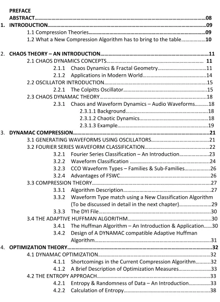
The following schematic is an example using an NPN transistor in the common base  configuration. [2] 

Figure 4 – NPN Transistor ‐ CB 

Frequency of oscillation is roughly 50 MHz:    

The follo Figure 5 –                      

The bipo gain at th The idea

Given the real circu transisto

ANALY

One met neglectin oscillatio the frequ An ideal  the sectio

wing schem – NPN Trans

lar transisto he oscillation

l frequency 

e values in t uit will oscilla

r and possib

YSIS 

hod of oscill ng any reacti on is possible uency of osc

model is sho on above. Fo

atic is a com sistor ‐ CC 

or could be r n frequency of oscillation

[2 he circuit ab ate at a sligh bly other stra

Fig lator analysi ive compone e. This metho

illation.  own to the r or initial ana

mmon collect

eplaced with . 

n is given by

] 

bove, the eq htly lower fre

ay capacitan

gure 7 ‐ Colpi is is to deter ents. If the im od will be us

right. This co alysis, parasi

tor version o

h a JFET or o

y this equatio

uation pred equency due nces. 

itts oscillato rmine the inp

mpedance y sed here to d

onfiguration  tic elements

of the same 

other active 

on: [2] 

icts a freque e to junction

  or model[2]

put impedan yields a nega

determine c

models the  s and device

oscillator:[2

device capa

ency of roug n capacitanc

nce of an inp ative resistan conditions of

common co e non‐linearit

2] 

ble of produ

hly 58 MHz. ces of the 

put port  nce term, 

f oscillation 

ollector circu ty’s will be 

ucing 

 The 

and 

ignored.  approxim Ignoring   

Where v1  

v2 = i2Z2[2  

Where Z2

currents:  

i2 = i1 + is

Where is 

Where g

Where Z1  

Zin = Z1 +   

The inpu which is   

Rin = gmZ

If Z1 and 

impedan  

If an indu negative  frequenc  

These terms mations, acce the inducto

[2]  1 is the input

2] 

2 is the impe

: 

is the curre

m [2]is the tr

  1 is the impe

Z2 + gmZ1Z2 

t impedance proportiona

Z1Z2 

Z2 are comp

ces for Z1 an

uctor is conn resistance i cy of oscillat

s can be incl eptable com r, the input 

t voltage an

edance of C2

nt supplied 

ransconduct

edance of C1

e[2] appears al to the prod

plex [2]and o nd Z2 are sub

nected[2] to  s greater tha ion is as give

luded later i mparison with

impedance c

d i1 is the inp

. The curren

by the trans

tance of the 

1. Solving for

s as the two  duct of the t

of the same s bstituted, Rin

the input, t an the resist en in the pre

n a more rig h experimen can be writt

put current.

nt flowing int

sistor. is is a d

transistor. T

r v2 and subs

capacitors i two impedan

sign, Rin will  n is 

he circuit wi tance of the  evious sectio

gorous analy ntal results is

en as 

 The voltage

to C2 is i2, w

dependent c

The input cu

stituting abo

n series with nces: 

be a negativ

ill oscillate if inductor an on. 

ysis. Even wit s possible. 

e v2 is given b

hich is the s

current sour

rrent i1 is giv

ove yields 

h an interest

ve resistance

f the magnit nd any stray 

th these 

by 

um of two 

rce given by

ven by 

ting term, Ri

e. If the 

ude of the  elements. T

in 

For the e roughly 4  

This valu oscillatio capacitan If the two becomes and a neg  

Rin = − gm

2.3 CH

2.3.1 C

2.3.1.1

2.3.1.2

Chaotic s been sho provide e typical ch from a st

example osci 40 mS. Given

e should be  on is more lik

nce. 

o capacitors s a Hartley o gative resist

mω2L1L2 

AOS DYN

CHAOS W

1 BACKGR

AC (dy‐NAM‐ on of the pro that can be  of producing e, such as th oscillation th to specify th size of the d oscillator’s a

g arbitrary d al images [1] the potentia sms. 

2 CHAOTI

systems have own to 

efficient ope haotic system tandard elec

illator above n all other va

sufficient to kely for large

 are replace scillator. In t tance given b

NAMAC T

WAVEFORM

ROUND 

‐ac) stands f ocess lies in  governed by g diverse wa hat derived f hat matches  e initial cond digital seque

bility to prod igital sequen . We introdu al it has for c

C DYNAM

e been studi

eration [2] an m is the Colp ctrical circuit

e, the emitte alues, the in

o overcome  er values of t

d by inducto that case, th by: [2] 

HEORY(A

M DYNAM

for dynamics the realizat y mathemat aveform shap

from image d it within an  ditions need ence, compre

duce diverse nce segment uce this new comparative

MICS 

ied for years

nd have app pitts oscillato t architectur

er current is  put resistan

any positive transconduc

ors and mag he input imp

Applicatio

MICS – A

s‐based algo ions that (a) ical expressi pes. The pre data, can be acceptable  ded to repro ession is ach e waveform 

ts. There are w nonlinear d e improveme

s in physics a

plications in v or. These se re that is use

roughly 1 m nce is roughly

e resistance i ctance and/o

gnetic coupli pedance is th

on Theory

UDIO WA

orithmic com ) chaotic osc ions, and (b) emise is this:  replaced by error toleran duce the ch hieved. Furth

shapes, we  e a number o dynamics‐ba ents given a 

and enginee

various engi ts of equatio ed widely in 

mA. The trans y[2] 

in the circuit or smaller va

ng is ignored he sum of th

y) 

AVEFORM

mpression. Th cillators are d ) chaotic osc

 a segment  y the initial c

nce. If the si aotic oscillat her, if we im

increase the of compress ased algorith deeper stud

ering. Chaoti

neering disc ons are actu engineering

sconductanc

t. By inspect alues of 

d, the circuit e two induct

M

he basic  dynamical  cillators are 

of a digital  conditions of

ze of the da tion are sma mprove the 

e probability sion algorith hm and attem dy of its 

c processes 

ciplines [3],[4 ually derived g [5]. The 

ce is 

tion, 

t  tors 

f a  ta  aller 

y of  ms  mpt 

have 

equation form: [4]

Where ic 

are empi we integ get a set  state‐spa waveform

2.3.1.3

Our first  subseque were suf image va definition the origin PSNR = 

ns are a three  

is the forwa irically deriv

rate these e of time dep ace plot as se ms in figure 

3 FULL IM

example in  ent decomp ficiently diff ariation. For  n of the mea nal image an

√

e‐dimension

ard transisto ed factors fo equations for pendant wav een in the fi

1(b)[4]. 

MAGE EXA

Figure 4, sho ressed versi ferent than e

each case[4 an square er nd   is the n  [8]. We s

nal set of no

LdiL dt V

C dv dt Cdv

dt

or collector c or the transi rward in tim veforms iL t

gure 1(a)[4]

AMPLE 

ows the com ons for diffe each other in 4] we ran the

rror that is  M new decomp

how the ave

nlinear ordin

v R

iL  

v R Cdv

dt iL

current defin stor and RL i

me from a set

, V t , V t

 and section

mparisons of  erent compr

n order to de e algorithm f

MSE =  ∑ pressed imag erage values

nary differen

RL iL 

V_EE

R  

i   ned by 

s the series  t of initial co

t  that can b ns of the cor

f two differe ession ratios emonstrate  for Ns = 16, 

  ∑  

ge, and the p  for these m

ntial equatio

1

resistance o onditions  iL

e plotter ve responding t

nt images w s. We chose  the algorith Ns = 32, Ns =

, ,

peak signal t measures for 

ons that hav

1  where γ a of the induct

, V , V  w rsus time or time‐depen

with their  two images hms viable gi = 64. We use

, where  to noise ratio

R, G and B. e the 

nd α  tor. If  we  r as a 

dant 

s that  iven  e the 

Figure 8. Image Compressed using the DYNAMAC algorithm at three different compression  rations showing the mean‐square error and peak signal‐to‐noise ratio. 

OTHER DATA TYPES 

It is clear that given digital sequences with smooth relationships, the DYNAMAC algorithm will  work. The compression metrics will be different depending on the format of data such as Audio,  Video or Image. For example, for 16‐bit stereo audio files there four components to the D‐bite  D = [D1, D2, D3, D4], with there being three 16‐bit integers and one 4‐bit integer, for a total of  52 bits. A 64‐point sequence for one channel would be 1024 bits, so the compression ratio  would be 19:7:1. 

3. DYNAMAC COMPRESSION 

3.1 GENERATING WAVEFORMS USING OSCILLATORS 

Using a typical Oscillator such as the Colpitts Chaotic Oscillator several waveforms are  generated to contribute in forming the CCO Matrix (See 2.2 for more details). The non‐linear  characteristics of a Chaotic oscillator are our objective for using such a system. 

Figure 9 ‐ STATE SPACE PLOT[4] 

The time dependant waveforms generated using the Oscillator are then arranged in the CCO  Matrix and through several techniques like intermultiplication or replacement of a certain set  from the whole row to get different variations of the waveforms. These 32 different types (12 +  Variations) constitute the CCO Matrix. 

Integrati we get a  plot or as  

3.2 FO

3.2.1 F

Chaotic o fact by u the trans chaotic o calculatin waveform and com having a  sequenti

ng the Oscill set of time  s the corresp

URIER SE

FOURIER S

oscillations t utilizing sets  sform proce oscillations, 

ng the chao ms are pre‐c

bination.  Th 16‐bit reso al  search  p

  Fig

lator equatio dependant w ponding tim

ERIES WA

SERIES CL

tend to have of these wa ess.  Essentia and the com otic oscillatio calculated a here are thi olution.   The

process  that

gure 10 ‐ TIM

ons forward waveforms t e dependan

AVEFORM

LASSIFICA

e a high mea aveforms in  ally, it is a c mbination of ons from in nd stored. T rty‐two diffe e best match t  seeks  out

ME DEPENDA

 in time from that can be p nt waveform

M CLASSIF

ATION – I

sure of time the CCO ma ollection of  f those wave

itial conditio This also allo erent wavef

hing wavefo t  the wavef

ANT PLOT O

m a set of in plotted vers  as seen in t

FICATION

INTRODU

e diversity.  T atrix.   The C digital wave eforms in di ons and ma ows greater orms, each  orm from th

form  with 

F WAVEFOR

itial conditio us time or a he figures a

UCTION

The D‐transf CCO matrix i eforms deriv

fferent man athematical  r variation in

comprised o he CCO mat

minimal  er

RMS[4] 

ons  iL , V , s a state‐spa bove.  

7]

form exploit is at the hea ved from va nners.  Inste expressions n oscillation  of 216 data p

rix is found  ror.   The  F

, V   ace 

procedure is an attempt to reduce the number of search iterations needed to find the optimal  waveform.

3.2.2 WAVEFORM CLASSIFICATION 

Fourier series waveform classification (FSWC) is based upon the fundamental notion of the  Fourier series decomposition of waveforms, namely,  

∑

+ +

=

1

1 1

0 cos sin

) (

n

n

n n t B n t

A A

t

v ω ω ,   (8) 

where An and Bn are the Fourier coefficients for the sine‐cosine form of the series.  A digital 

sequence can be generated from the coefficients.  If we designate M to be the number of bits  for the quantization of each coefficient[17], and N to be the number of coefficients used for An 

and Bn, then we designate a given encoding as M‐N FSWC. Suppose we have the waveform 

shown in fig. 3. This waveform could be pulled from the CCO matrix, or could be part of a digital  audio, video, or image set of data, or any other digital sequence for that matter.   

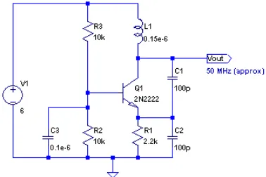
Fig. 11 ‐  Digital waveform used to demonstrate a 3‐3 FSWC decomposition 

The corresponding [18]3‐3 FSWC decomposition is shown in fig. 4. There are a total of six  coefficients each having a 3‐bit resolution, therefore resulting in an 18‐bit sequence for this  waveform, that is, 

3 3 2 2 1

1 B A B A B

Ab b b b b b

b= .   Just as the accuracy of the series increases with the 

number of coefficients, so does the uniqueness of the binary sequence as its length increases. 

  . 

Fig.12. 3‐3 FSWC sequence showing the formulation of the 18‐bit sequence b =  100010110010010010[17]. 

3.2.3 CCO WAVEFORM TYPES – FAMILIES & SUB‐FAMILIES

oscillation type number 4, while fig. 14 shows their respective 3‐3 FSWC coefficients and 18‐bit  binary sequences.  

Fig. 13. Three 128‐point waveforms [17]extracted from type number 4 of the CCO matrix. 

Fig.14. The FSWC decomposition [17]of each waveform from fig. 5, and their corresponding 18‐ bit binary sequences. 

3.2.4 ADVANTAGES OF FSWC 

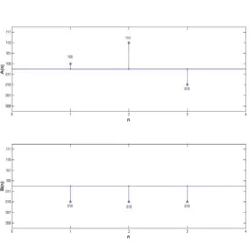
according to the 10‐bit family structure.  Fig. 15 shows a histogram, or FSWC spectrum, of the  number of CCO matrix waveforms that fall into the 1024 different families for Nc = 128.  This 

spectrum indicates the total number of waveforms in a given 10‐bit family that are necessary to  search through in order to find the best match.  In this case the maximum number of elements  in a given family is 1,570, in contrast to having to search through 65,336 waveforms using the  old method. In some cases, a particular family may have no members. In that case the nearest  neighbor (or extended family) is used for the search criteria. 

Fig.15. 3‐3 FSWC spectrum showing a 10‐bit pre‐classification family profile the CCO matrix  where Nc = 128. 

3.3 COMPRESSION THEORY 

3.3.1 ALGORITHM DESCRIPTION 

digital sequence, such as that derived from audio, video, and image data, can be replaced by  the initial conditions of a chaotic oscillation that matches it within an acceptable error 

tolerance. Symbolically, we can describe DYNAMAC operator as  −1

D , where   is the original  digital sequence, C is the combined chaotic Oscillation matrix, and   is the matrix ordering  sequence. If we call l(.)a length function, then if l

( ) ( )

reproduce the digital sequence by x′=D−1

(

)

Ns

ε , where Ns is the length of the digital sequence. If E = 0, 

then the compression is lossless.   

The key to high compression ratios and high image quality is to the chaotic oscillator’s ability to  produce diverse waveform shapes. By doing so, we increase the probability of matching 

arbitrary digital sequence segments.  The images that we examine are in bitmap format, where  each R,G, and B component is specified by 8‐bit integers. So then, each segment of the image is  8x3xNs bits long. For this particular image each 64‐point [4]segment represents 1,536 bits   

  Figure 17. DYNAMAC™ [4]compression engine block diagram. 

3.3.2 WAVEFORM TYPE MATCH USING NEW CLASSIFICATION 

ALGORITHM 

The key to the algorithm is in finding a proper match to the input digital sequence xp[n] using a  combined chaotic oscillation represented by c[n].  Figure 3 is a block diagram of the algorithm.   The combined chaotic oscillation matrix, or CCO matrix, stores 32 oscillation types that can be  accessed by submitting a type number, Nt, an oscillation starting point, Ni, and an oscillation  length, Nc.  The resulting chaotic oscillation will then be decimated [17]down to the length of  xp[n]. This new oscillation will be called cn[n]. The RMS error between xp[n] and cn[n] is  calculated.  Oscillations having the smallest error value will be chosen as replacements for  xp[n]. The information needed to reproduce the chosen chaotic oscillation can be distilled  down to two 16‐bit integers and one 4‐bit integer we call digital bites, or D‐bites. Specifically, D  = [D1, D2, D3]. Since there are three digital sequences connected with an RGB image, and each  component requires its own D‐bite, DR, DG, DB, then each image segment requires 108 bits. In  this example, the compression ratio is 1536:108 or 14.2:1. The new file, which we’ve called .dyn  files, are stored as [HEADER],DR1,DG1,DB1,DR2,DG2,DB2,DR3,DG3,DB3,…,DRN,DGN,DBN, where N = 

LxW/Ns.   

With the new classification algorithm, instead of going through each and every single piece of  waveform data, if the input waveform can be identified as belonging to a particular class, only  those waveforms have to be scanned for the closest match. This procedure due it repetitive  nature can also yield 2‐3 classes which have similar characteristics as the input waveform and  hence when there are more options to choose from, there is a better match. 

Digital Sequence Initialization

file

Sequence

Parser

C

Combined Chaotic Oscillation Matrix CO

Decimator

Scaling Δ

∑

1

f x

Ns _p  

Input Buffer

x[n]

xp[n]

Ns _Ns

cn[n]

ε[n]

c[n]

Nc

εf

D-bite

xpmin, xpmax

Nt Ni Nc

D = [D1,D2,D3]

Fixed Storage

Ns Ns

Ni Nt

Nc

3.3.3 THE DYI FILE 

The amount information needed to recreate the chosen chaotic oscillation can be distilled  down to two 16‐bit integers and one 4‐bit integer we call digital bites, or D‐bites. The D‐bites  contain three different digital sequences corresponding to the colorspace RGB respectively.    

D = [D1, D2, D3] 

Every single one of these components would require its own D‐bite i.e D1 (Red), D2(Green),  D3(Blue) for representation. The size of each of the segments would be 108 bits. For e.g. if the  compression ratio is 1536:108 (see example in section 2.3.1.3) or 14:2:1, the new file which we  would call as the DYI (DYNAMAC Image File) file would be stored as the following sequence.   

 [HEADER],DR1,DG1,DB1,DR2,DG2,DB2,DR3,DG3,DB3,…,DRN,DGN,DBN, where N = LxW/Ns.     

3.4 THE ADAPTIVE HUFFMAN ALGORITHM 

3.4.1 THE HUFFMAN ALGORITHM – AN INTRODUCTION & 

APPLICATION 

In general parlance, Huffman Coding  is an Entropy Coding Algorithm[2] which results in a  lossless data compression. In this particular technique we use a variable length code table for  encoding a source symbol (such as a character in a file) where the variable‐length code table  has been derived in a methodical way based on the estimated probability of occurrence for  each possible value of the source symbol. 

In other words [6]for any code that stands unique for more than one case, meaning that the  code is uniquely decodable, the sum of the probability of occurrences across all symbols is  always less than or equal to one. Generally the sum is strictly equal to one; as a result, the code  is termed a complete code. If this is not the case, a similar code can be quite easily derived  which has an equivalent code. This is done by adding extra symbols (with associated null  probabilities), to make the code complete while keeping it biunique. 

A commercial study would reveal the effectiveness of the Huffman algorithm to double or more  the compression ratio of an already existent compression algorithm without inducing any losses  in the input data. Also due to its tree/ladder structure, the decoding of such an algorithm would  be of lower complexity as well. 

3.4.2 D

ALGOR

An adapt of ladder algorithm

For e.g. if adding a  inducing  any alien

DESIGN O

RITHM 

tive version  r elimination m 

f the stand a Huffman blo any losses i n substantial

F

OF A DYNA

of the HUFF ns to facilitat

alone Compr ock to the co n the data. B  loss in the D

Figure 42 – A

AMAC CO

FMAN algorit te a ‘doublin

ression ratio ode will dou By lossless, i DYI data 

Addition of a

OMPATIB

thm[6] was d ng’ of the co

o achieved b uble the com n our contex

a Huffman M

BLE ADAP

designed for mpression r

y DYNAMAC mpression rat xt we mean 

Module to DY

PTIVE HUF

r DYNAMAC  ation alread

C turns out a tio of the alg that it woul

YNAMAC 

FFMAN 

with lower  dy achieved b

around 1:8,  gorithm with

d not introd level  by 

4. OPTIMIZATION THEORY 

4.1 DYNAMAC OPTIMIZATION 

4.1.1  SHORTCOMINGS OF THE CURRENT COMPRESSION ALGORITHM 

After validation and test of the efficacy of our compression algorithm, it was obvious to  ascertain, following a conventional thought process, the advantages and the disadvantages of  our current algorithm. That would in‐turn lead us to a crossroads of further research and  investigation into fields such as quality improvement, speed of the algorithm and compression  ratio. 

After preliminary testing, various parameters were marked out which were more or less eligible  for improvement. Some of those parameters are mentioned as below. 

1. The Compression ratio, although impressive in its own right, could be increased twin‐fold of  more using one of the more conventionally used add on “Lossless” compression techniques  such as Huffman, Lempel‐Ziv etc. Is there a possibility of an adaptive version of such an  algorithm to asset our compression? 

2. If we are measuring improvement, will a passive measure such as PSNR suffice?   

3. The PSNR measure being passive could only be used for “Post‐Analysis”. In short it would  show post compression whether the algorithm was improved due to arbitrary changes in  the Matrix or the algorithm itself, but there lies the obvious disadvantage. It cannot “drive”  the compression to improvement. What are the measures which can be considered for such  a task? 

4. The arbitrary arrangement of waveforms generated from various oscillators, did in‐fact give  us compression, but there being a lack of order in their arrangement or a mathematical  motive, there is a definite possibility that given a measure for driving the compression  algorithm, there would be a set of new waveforms which would perform better than the  current set. If this line of thought is indeed true, what are the plausible methods for  generating these waveforms. 

5. A simple Histogram analysis would show that there are certain types of waveforms which  don’t get utilized in the compression process compared the other ones. If these are termed  as under‐utilized or non‐utilized waveforms, what kind of methods can be employed for  reducing such under‐utilization? 

7. The current scanning process, where the algorithm scans the entire CCO matrix for the most  appropriate match for the image waveform, results in scanning the matrix individually every  time for every single image waveform. The complexity of such a scanning processing is a  little too large and can be optimized. 

7.1    Is there a possibility of an alternate scanning algorithm, if the image waveform  “TYPE” is detected before‐hand? 

7.2   Would “CLASSIFICATION OF WAVEFORMS IN FAMILIES” and re‐structuring the  CCO Matrix improve the speed of the algorithm, as instead of searching the  whole matrix, the algorithm has to search only one family post detection of  image waveform type? 

8. Is there a possibility of certain waveforms performing better for a certain set of images? If  there exists such a dependency, does the current configuration of CCO waveforms suffice  and if not what kind of waveforms are necessary for fulfilling such dependencies? 

4.1.2 A BRIEF DESCRIPTION OF THE OPTIMIZATION MEASURES 

The Optimization measure per se represents those measures which would be independently  able to ascertain certain parameters pivotal for Compression algorithm Pre/Post Compression.  Some of the properties these "measures" were intended to display were as follows. 

For ease of explanation, let’s denote our measure as “

η

”.

•

• The measure should be an independent constant with respect to the compression  algorithm in order to facilitate a stand‐alone analysis of the compression algorithm or  the Compression Matrix. 

• The measure should perform in accordance to one of the Post analysis tools for quality  such as PSNR to reconfirm its validity for the analysis case. 

4.2 THE ENTROPY APPROACH 

4.2.1 ENTROPY & RANDOMNESS OF DATA – AN INTRODUCTION 

INFORM

In inform of the un  

It can be  commun fundame commun message   Equivalen recipient The conc Commun

DEFINIT

The infor values {x

Where[6 I( a p

CHARAC

MATION

EN

mation theor ncertainty as

interpreted nicate the tru

ental mathem nication: the 

 out of all th

ntly, the Sha t is missing w cept was intr nication".[6] 

TION

rmation ent

x1...xn} is defi

6] 

X) is the info nd 

(xi) = Pr(X=x

CTERIZATIO

tion entropy

ty[6]  he measure y a very sma

NTROPY

y, the SHAN

ssociated wit

d as the aver ue value of t matical limit shortest ave he possibiliti

annon entro when they d roduced by C

tropy of a d ined to be 

ormation co

i) is the prob

ON

 can be char

an

 should be c all amount s

NNON ENTRO

th a random

age shortest the random v t on the best

erage numb es is the Sha

py is a meas o not know t Claude E. Sh

iscrete rand

ntent or self

bability mass

racterized by

nd 

continuous — hould only c

OPY [5]or IN

m variable. 

t message le variable to a t possible los er of bits tha annon entro

sure of the a the value of annon in his

dom variable

f‐informatio

s function of

y the followi

— i.e., chang change the e

NFORMATIO

ength, in bits a recipient. T ssless data c at can be se

py.[6] 

average infor f the random s 1948 pape

e X, that can

on of X, whic

f X. 

ing desidera

)[5

ging the valu entropy by a

N ENTROPY

s, that can b This represe compression nt to comm

rmation con m variable. 

r "A Mathem

n take the r

[2] 

ch is itself a r

ta:[6] 

5] 

ue of one of   small amou

Y[5] is a meas

e sent to  nts a  n of any 

unicate one 

ntent the 

matical Theo

range of pos

random vari

the probab unt. 

sure 

ory of 

ssible 

iable; 

Symmetr T Maximum If e Additive[ T re T It sy A w th th o Fo T Shannon

where K 

EXAMP

ry[6] 

he measure 

m[6] 

f all the outc ntropy incre

[6] 

he amount  egarded as b his last func t demands t ystems if we Assume that  we mentally  he entropy c he probabilit

f boxes.  or positive in

rivially, this 

 shows that 

is a constan

LE

should be u

comes are e eases with th

of entropy being divided ctional relati

hat the entr e know how  we have an  divide this e can be calcu

ty of finding

ntegers bi w

also implies [6] 

any definiti

t correspond

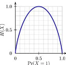
      Figu it co

unchanged if

equally likely he number o

y should be d into parts. onship char ropy of a sys

the sub‐syst ensemble o ensemble in ulated as a s

g oneself in 

where b1 + … 

 that the en

on of entrop

[6] 

ding to a cho

re 18 – Entr ming up hea

f the outcom etc. 

y, then entro of outcomes

e the same   

acterizes the stem can be tems interac of n element nto k boxes  um of indivi that particu

+ bk = n, 

tropy of a ce

py satisfying

oice of meas

opy of a Coi ads 

mes xi are re‐

opy should b . 

independe

e entropy of e calculated  ct with each  ts with a unif

(sub‐system idual entrop ular box PLU

ertain outco

g these assum

surement un

in toss as a f

‐ordered. 

be maximal.

ntly of how

f a system w from the en other.  form distrib ms) with bi e

pies of the b US the entro

me is zero: 

mptions will 

nits. 

function of t

. In this case

[5

w the proce

with sub‐syst ntropy of its

ution on the lements in e oxes weighe py of the sy

[6] 

be of the fo

the probabil e, the 

] 

ess is 

tems.  s sub‐

em. If  each,  ed by  ystem 

orm: 

[2]Consid

The entr (that is, i uncertain of the co

However likely to  average e

The extre uncertain

PROPER

The Shan

• A • It

ASPECT

DATA C

LIMITA

Although source, t A source symbol is

der tossing a

opy of the u if heads and nty as it is m oin delivers a

r, if we know come up th each toss of

eme case is  nty. The ent

RTIES

nnon entrop

Adding or rem

t can be conf

TS 

COMPRE

effectively  sion possibl ffman, Lemp ms is often u

ATIONS O

h entropy is his informat  that always s depends o

a coin which

unknown re d tails both  most difficult

a full 1 bit of

w the coin is han the othe f the coin de

that of a do ropy is zero:

y satisfies th

moving an ev

firmed using

SSION 

bounds the e, which ca pel‐Ziv or ar sed as a rou

OF ENTRO

s often used tion content s generates  on the alpha

 may or may

sult of the n have equal  t to predict t f information

s not fair, th er. The redu

livers less th

ouble‐heade : each toss o

he following 

vent with pr

g the Jensen 

e performan an be realize

rithmetic cod ugh estimate

OPY AS IN

d as a char t is not abso the same sy bet. Conside

y not be fair

next toss of  probabilities the outcome n.[2] 

ere is less u uced uncerta han a full 1 b

d coin which of the coin d

properties:

robability ze

[

inequality t

nce  of the  ed in theory ding. The pe e of the entr

NFORMAT

racterization lute: it depe ymbol has e er a source t

. 

the coin is  s 1/2). This  e of the next

ncertainty.  ainty is qua bit of inform

h never com elivers no in

ro does not 

[2]. 

that 

strongest  y by using t erformance o

opy of a blo

TION CON

 of the info ends crucially ntropy of 0, that produce

maximized  is the situat t toss; the re

Every time,  ntified in lo ation. 

mes up tails.  nformation. 

contribute t

lossless  (or  he typical s of existing d ck of data. 

NTENT

ormation co y on the pro  but the def es the string

if the coin i tion of maxi esult of each

one side is  ower entrop

Then there 

to the entro

[2]. 

nearly  loss set or in pra data compre

ontent of a  obabilistic m finition of w g ABABABAB

s fair  mum  h toss 

more  y: on 

is no 

in which  letters a sequence entropy r

However become  not know every bo If there  probabili correspo book wh books, bu of langua knowing  that the  theoretic of a seq program  rate of a such prog

DATA

A

A commo source (e

where pi

selecting

rate is: 

where i  previous 

For a sec

A is always  s independe e is consider rate is 0 bits

r, if we use  artificially lo wable exactl ok ever pub are N publi ity of each b onds to assig henever one ut it is not so age in gene

the probab complexity  cal generaliz quence inde for a univer a sequence f gram, but it 

AS

A

MARK

on way to de each charact

i is the proba

g a character

is a state (c character (s

cond order M

followed by ent, the ent red as "AB A s per charact

very large  ow. This is b ly; it is only blished as a s

ished books book is 1/N, gning each b e wants to r o useful for  eral: it is no ility distribu of the proba zation of this ependent of

rsal compute for a given 

may not be

KOV

PROCE

efine entrop ter is selecte

ability of i. F r is depende

certain prece s). 

Markov sourc

y B and vice v tropy rate o AB AB AB AB

ter. 

blocks, the ecause in re y an estimat

sequence, w s, and each 

 and the en book a uniqu refer to the

characterizi ot possible t ution, that is abilistic mod s idea that a f any partic er that outp model, plus   the shortes

ESS

py for text is ed independ

[6] 

For a first‐or ent only on 

eding chara

ce, the entro

versa. If the of the sequ B..." with sym

n the estim eality, the pr te. For exam with each sym

book is on tropy (in bit ue identifier  book. This  ng the infor to reconstru , the comple del must be  allows the co cular proba puts the sequ

the codebo st. 

s based on th ent of the la

rder Markov the immedi

cters) and p

opy rate is 

 probabilisti uence is 1 b mbols as tw

mate of per‐ robability dis mple, suppos mbol being t ly published ts) is ‐log2 N

r and using  is enormou mation cont uct the book ete text of a considered. onsideration bility mode uence. A cod ook (i.e. the

he Markov m ast character

v source (on iately preced

[6] 

pi(j) is the p

ic model con bit per char wo‐character 

character e stribution of se one cons the text of a d once, the 

N. As a pract it in place o usly useful f tent of an in k from its id all the books . Kolmogoro n of the info

l; it conside de that achi

 probabilisti

model of tex rs), the bina

e in which t ding charact

robability o

nsiders�