Some problems in recursive estimation

TANIA PRVAN.

JULY.

1987.

Tania Prvan: Some Problems in Recursive Estimation, Ph.D thesis 1987

p.v 1-2 p.3 1-9 p.5 1 7 p.21,22 p.22 1-8 p.26 1-8 p.32

1 6 1-4 p.34 1-8 p.35

p.51 1-5 p.78

p.81

p.85 1-3 p.93 1 12 p.103 1 12 p.104 1 8 p.107 1-7 p.116 1-0

p.123 1-7 p.127

Errata and Addenda

pis the dimension of the state space 2

x{t₁)-Jf{O,, I) {also p.78, 1-2 and p.109, 1 6} ... requires that f{t) be

ffiROLLARY

p

=

{WTQ-lW+R-1)-lWTQ-ly ... are given

equation should be {2.3.11) ... {2.3.3)

... {2.3.11)

Also Weinart, Byrd and Sidhu {1980) T{t.,t.

1). u{t.,t. 1) correspond to T., u. in {2.3.3)

1 1- 1 1- 1 1

... denote

Wecker and Ansley { 1983) is a general reference to this chapter. An extension in a somewhat different direction is given in Kohn and Ansley {1985), but there is some overlap with the results presented here.

in {6.2.9) T{t.

1.t.), in {6.2.11) 1+ 1

... Problem 2.3.1 and Theorem 2.3.3 ... {6.5.12)

... {7.2.10) ... Recollect

f2{ t.

1 , t. ) ,

a2r...

1+ 1

the term marginal likelihood is also used

a similar result is given in Ansley and Kohn {1985) {also p.121, 1 O}

dw/ds

DECLARATION.

Much of the material in Chapters 5, 7, 8, and 9 is contained in Osborne and Prvan (1987a), (1987b) and Prvan and Osborne (1987) , and represents joint work with my supervisor M.R. Osborne. Except where otherwise stated, the work presented in this thesis is my own.

ACXNOWLEOCEMENTS.

I thank my supervisor Mike Osborne for having me as a student,

for his assistance and encouragement throughout my course. I also thank Robert Kohn and Craig Ansley for making their results freely available to Mike Osborne and thank Peter Thompson for some helpful

ABSTRACT.

Smoothing Splines provide curves which smooth discrete, noisy data. The connection between Smoothing Splines and the solution to a

particular stochastic differential equation conditioned on all of the available data has given rise to new approaches for obtaining such smoothed curves. These approaches exploit a state space formulation that is provided by the solution to the stochastic differential

equation and the observation equation. This stochastic setting has the added advantage that it permits confidence intervals to be attached to Smoothing Splines. A new approach for determining the smoothing parameter based on maximum likelihood estimation has also resulted. The Kalman Filter, the Fixed interval, Discrete time Smoother and Interpolation Smoother are invaluable tools in this stochastic approach. They are introduced in Chapters 2 and 3 and stable recursive implementations of t:hem are the main thrust of Chapters 4 and 5.

Chapter 6 extends Wecker and Ansley's (1983) stochastic approach to Lg Smoothing Splines while Chapter 7 presents other

approaches.

stochastic

In Chapter 8 a generalization of the stochastic formulation of Smoothing Splines is developed. This framework produces smoothed curves which can possess less than the usual order of continuity at

the data points.

Numerical algorithms for Generalized Smoothing Splines and the inherent sensitivity of these algorithms are considered in Chapter 9.

with which other algorithms are compared. Numerical results which support the conclusions based on the sensitivity analysis of the algorithms are presented.

NOTATION.

A convention followed in this thesis is that capital case letters are reserved for matrices and bold lower case letters denote vectors unless otherwise stated. The sign _{indicates equal by} definition ·. A list of notation encountered in this thesis is given below.

ffi == the set of real numbers O(•) == is order of(•)

11 • 11

2 : = Euclidean norm - == is approximately

- N(µ, ~) == is normally distributed with meanµ and covariance

1

0 _{ij . -}. - 0 _{ij -}

=

{01

e. _l == vector with 1 in i'th position and zeroes elsewhere

x. : = x( t.)

l l

z. ·- z(t.)

l l

u. . - u( t. , t.

1)

l l

1-c. ·- c(t.)

l l

Yi ·- y(ti)

n. . - n(

t .. c. 1)

l l

1-== x(t. lk)

l

== S(tjk) the covariance of x(tlk) unless otherwise stated CV== Cross Validation

GCV ·- Generalized Cross Validation GLS ·- Generalized Least Squares LS== Least Squares

RSS

==

Residual Sum of Squares

RQ

==

Rayleigh quotient

dp

nP

==

dtp

L+ ·- formal adjoint of the differential operator L

tr

.

.

-

trace

a. (C) .

.

-

_{i'th largest singular value of C}

l

cond{C)

==

_{condition number of C}

+

0 where

o>O

and 0 -+ 0

t

.

.

-

t +

DECLARATION.

ACKNOWI..E]X;EMENTS.

ABSTRACT.

N

OTATION.

TABLE OF CONTENTS.

C1IAPIER 1 : INTRODUCTION.

1.1

Smoothing Splines.

1.2 Cubic Smoothing Splines.

1.3 Choosing the smoothing parameter.

1.4 Material covered in this thesis.

C1IAPTER 2: IBE KALMAN FILTER.

2.1 Introduction.

2.2 Some Estimation Problems.

2.3 The Kalman Filter.

aIAPTER 3: SMOOTIIERS.

3.1 Introduction.

3.2 Discrete time, Fixed point Smoother.

3.3 RTS Smoother.

3.4 Interpolation Smoother.

ii.

iii.

iv.

vi.

1 . 3.

7. 10.

13.

17. 23.

34.

CHAPTER 4: IMPLEMENTING TIIE KALMAN FILTER.

4.1 Introduction.

4.2 Covariance and Information Filters.

4.3 Information Filter.

4.4 Covariance Filter.

45.

47.

48.

55.

CHAPTER 5: A SQUARE ROOT FIXED-INTERVAL. DISCRITE TIME SMOOTHER.

5.1 Introduction. _62.

62.

64.

70.

72. 5.2 Preliminaries.

5.3 Bierman's Algorithm.

5.4 A square root algorithm.

5.5 Examples.

CHAPTER 6 : EXTENDING TIIE ANSLEY AND WECKER APPROACH TO SMOOTHING

SPLINES TO HANDLE LG SMOOTHING SPLINES.

6.1 Introduction.

6.2 State space formulation.

6.3 Maximum Likelihood Estimation.

6.4 The Kalman Filter as a computational tool.

6.5 Smoothness properties.

CHAPTER 7: OTIIER SfOCHASfIC APPROACHES TO LG SMOOTHING SPLINES.

7.1 Introduction.

78. 80.

82.

85.

90.

96.

7.2 Stochastic derivation of generalized Reinsch algorithm. 97.

7.3 Working explicitly with the diffuse prior. 105.

7.4 An alternative derivation of Wienert. Byrd and

CHAPIER 8: GENERALIZED SMOOTIIING SPLINES.

8.1 Introduction.

8.2 Generalized Smoothing Splines.

8.3 Smoothness properties.

8.4 Roles that hand V play.

CHAPIER 9: ALGORITHMS.

9.1 Introduction.

9.2 Extending the Wecker and Ansley approach to handle

Generalized Smoothing Splines.

9.3 Information Filter algorithm for Generalized Smoothing

Splines.

9.4 Covariance Filter algorithm for Generalized Smoothing

Splines.

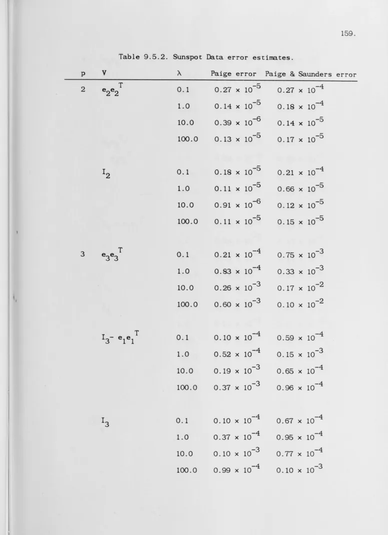
9.5 Numerical Results.

APPENDIX

1.

Lemma 1.

Matrix Inversion Lemma.

APPENDIX

2.

Proof of LEMMA 7.4.2.

APPENDIX

3: PERTURBATION RESlr~TS FOR

LEAST

SQUARES

PROBLEMS.

THEOREM 1.

THEOREM 2.

REFERENCES.

123.

126.

129.

132.

134.

136.

140.

148.

155.

165.

165.

166.

170.

171.

1.1. Smoothing Splines.

CHAPTER

1

INTRODUCTION

Suppose that the data y

1 .... ,yn are given at the data points t

1 .... ,tn respectively. In most situations the data y1, ... ,yn contain

errors. It isn't unrealistic to think of the data as being represented by a regression model

y. = f{t.) + E. ••

l l l i = 1, ... ,n, {l.1.1)

2

where E.. is normally distributed with zero mean and variance a . The

l

E.. can be thought of as ''noise'' and the function f{t) as the

l

·'signal''. If the underlying mechanism generating the data is not lalown then it doesn't make sense to prescribe a parametric form for f. A nonparametric form is desirable. This leads to the consideration of what sort of properties we would like f{t) to possess.

Fitting a polynomial of degree n-1 which interpolates the data is not desirable because it could oscillate wildly (see for example Atkinson ( 1978)) while the underlying function generating the data could be smooth. This suggests that a continuous piecewise curve might be desirable. It makes sense to prescribe the continuous piecewise curves between the points [t.

1.t.J, i=2, ... ,n. Interpolating the data 1- l

by a continuous piecewise curve is only useful if sufficiently accurate data is available. This is not always the case, so one desirable property of f ( t) is that it be free of the interpolation

integrable then minimizing the following functional

t

n n

1

(f(t.) - y.)2 + µ

f

. l 1 1

l=

(1.1.2)

over f where µ is constrained to be positive seems a useful

compromise. lne first term can be thought of as a measurement of the

approximation to the data and the second term as a penalty function

which prescribes the smoothness of the data. lne termµ is 1mown as

the smoothing parameter and can be thought of as controlling the trade

off between · ·smoothness· · and · • approximation to the data· ·.

Whittaker (1923) was the first person to perceive how to balance the

two conflicting goals of accuracy and smoothing. He used a sum of

squares of p'th differences in the penalty function and only

considered equally spaced data points. Schoenberg (1964) is

responsible for suggesting the functional {1.1.2). Reinsch {1967)

showed that the function which minimized (1.1.2) for a givenµ. in the

special case p=2. was a cubic piecewise polynomial with two continuous

derivatives at the data points t

2 . . . tn-l and zero second and third derivatives at the end points. For general p the function which

minimizes (1.1.2) is a piecewise polynomial of degree 2p-1 with 2p-2

continuous derivatives at the points t

2 . . . tn-l and zero p' th to (2p-l)'th derivatives at the end points. lnis function is kr..own as a

Smoothing Spline and is unique for given µ. lne problem of how to

estimate the optimal smoothing parameter µ will be addressed in

section 1.3.

Anselone and Laurent (1968) gave a general method for

constructing Splines and Smoothing Splines which exploited the Hil~ert

space setting they used.

Smoothing Splines as the mean of a posterior distribution given the

data under the assumption of an appropriately tailored form of the

prior distribution. Kimeldorf and Wahba (1970a). (1970b). (1971)

explored particular relationships between Bayesian estimation and

spline smoothing. Wahba (1978) provided a different formulation and

generalization of the result in Kimeldorf and Wahba (1971). She showed

that spline smoothing is equivalent to modelling the signal by the

stochastic differential equation

av'Adw(t) dt

where w(t) is a Wiener process with unit dispersion parameter (see,

for example, Billingsley (1979)) and A is a scale parameter

corresponding to the reciprocal of the smoothing parameterµ which is

to be determined. Let

be the vector of initial conditions on the above stochastic

differential equation. She shows that if x(t

1) is allowed to have a diffuse prior; that is, setting x(t

1) - N(o,..., 2

) and letting ...,2-+ 00 ;

then

f(t) = lim E{x(t)ly(t

1) .... ,y{t )}.

2 n

'"'( -+ (X)

A generalization of this result to smoothing splines that are not

piecewise polynomials was also developed in Wahba (1978).

1.2 Cubic Smoothing Splines.

In the literature the most important case of Smoothing Splines

used in practice is the Cubic Smoothing Spline (see, for example.

Spline is obtained by minimizing t

n 2 n 2

}: {f{ti) - yi) + µ

f

{f"{u)) du

i=l tl

F -

(1.2.1}

over f{t) for givenµ. It will be shown that the function f{t) which minimizes F is a piecewise cubic polynomial with 2 continuous derivatives at the points t₂ •... ,tn-l and zero second and third derivatives at the end points.

We will find

min F f{t)

by a standard variational argument. This is done by replacing f{t) by f(t)+en(t) in

(1.2.1)

where n is assumed to be continuously differentiable but otherwise arbitrary, differentiating the resulting expression with respect toe, then equating it to zero, and taking the limit as e ~ 0. It will be seen that to uniquely define the function f{t) some constraints have to be imposed.

Replacing f(t) by f{t)+en(t) in

(1.2.1)

yields

n 2

F - 2 (f{t.)+en(t.)-y.) +

. l

1 1 1

l=

t

µ fn(f' '(t)+en' '(t}}2dt. tl

Differentiating this expression with respect toe gives

Now

t

n n

!

dF = µ 2 de

f

n

I I ( t) ( f I I ( t )+ery I I ( t) }d t + }: n(t.)(f{t.)+en(t.)-y.).

. l 1 1 1 1

tl

1 11m _ . dF = µ 2 e--0 de

t

n

f

n

I I ( t) f I I ( t )d t +

tl

l=

n

2 n(t.){f{t.)-y.) . l 1 1 1

l=

and equating this expression to zero produces

-t.

n 1

µ }:

f

n

n' '(t)f' '{t)dt =}: n(t.)(y.-f{t.))

i=2 + ·-

·-

. l

1 1 1

which can be evaluated by integrating by parts to give

n n

µ i : / r y ' ( \ ) f ' ' ( \ ) - 11'(ti-l)f''(\~1)) - µ i:}11(\)f'''(t)

-t.

n 1

- n(ti_ 1)f' · '(t;_₁)) + µ 2

f

n(t)f( 4 ){t)dt _

i=2 +

n

t . _1-1

2 n(t.)(y.-f{t.)). {1.2.2)

. l 1 1 1

1=

We can't solve this uniquely without imposing some constraints. It is

desirable to make the integral vanish, since n(t) is assumed to be

arbitrary this can be achieved by making f(t) a cubic polynomial. Now

(1.2.2) can be rewritten as

n

µn'(t )f' '(t-) - µn'(t₁)f' '{t+

1) + µ 2 n'(t.){f' '(t~)-f' '(t:))

n n .

2 1 1 1

l=

- + n

- µn(tn)f'' '(tn) + µn(t 1)f'' '{t1) - µ 2 n(t.){f'' '(t~)-f' · '(t:))

.

2 1 1 1

l=

n-1

= n(t~)(y1-f{t 1)) + 2 n(t.)(y.-f{t.)) + n(t )(y -f{t )).

1 .

2 1 1 1 n n n

l=

This defines a unique cubic polynomial if the following constraints

are imposed

+

-f{t.) = f(t.)

l l i=2, ... , n-1.

f'(t:) = f'{t~) i=2, ... ,n-1.

l l

f I I ( t:) - f I I ( t ~) i =2 t • • • t n-1 •

l l

f I I ( tl) - f I I ( t ) = f I I I ( t ) = f I I I ( t ) = 0

n 1 n

f' I '(t:) - f' I '(t~) =

µ-1

(y. - f(t.)) i=l, • • • ,n.

l l l l

(1.2.3.a)

(1.2.3.b)

(1.2.3.c)

(1.2.3.d)

{1.2.3.e)

which implies that a convenient form of writing f(t) is

2 3

f(t) =a.+ b.{t-t.) + c.(t-t.) + d.(t-t.) .

l l l l l l l tE[t.,t. _{l 1-1}]

(1.2.4)

All that is left to do is determine the Cubic Smoothing Spline

coefficients. This is achieved by substituting (1.2.4) into equations

(l.2.3d) gives after simplification

where

h. - t. +l - t.

1 1 1.

d

.

₌

l

Ci+l - Ci 3h .

l

i=l ... n-1. _(1.2.5)

Inserting {l.2.4) into {l.2.3b) using {1.2.5) and rearranging it as an

expression for b. yields

l

b _{i -}

-a - a.

i+l 1

h.

1

i=l ... n-1. (1.2.6)

Putting {1.2.4) into {l.2.3b) and the utilizing {1.2.5) and {1.2.6)

after simplification produces

1 1

- a - (- +

h. i+l h. l

1

1-1

+ 3-h. le. _{1- 1 - .} 1 _{i=l ... n-1. {1.2.7)}

Substituting (1.2.4) into {1.2.3e) using (1.2.5) after simplification

yields

1

- C

-h. i+l

1 {1.2.8)

i=l ... n

Equations {1.2.7) and {1.2.8) can be rewritten in matrix form. They

become

(1.2.9)

and

1 -1

Qc

=

z.L

(y -

a)

_(1.2.10)

where T € Rn-2 x n-2 and Q € Rn x n-2 are tridiagonal matrices defined by

2

t .. ₁₁ = 3-(h. +

h.

1).

l

1-1

q. _1-1· - h _l ' q ₁₁ .. =

i-1 and

tii+l = ti+li

1 1

-(- + - )

h. l h. '

1- l

1

qi+li =

h ..

T

Y =(yl, ... ,yn).

T

a - (a

1 .... ,an).

The matrix Tis positive definite. Premultiplying (1.2.10) by QT and

using (1.2.9) gives

T 1 -1 1 -1 T

(Q Q +

2

µ T)c =

2

µ Q y (1.2.11)

which can be solved for c. Then from (1.2.10)

a= y - 2µ.Qc. (1.2.12)

Coefficients b. and d. can then be obtained from (1.2.5) and (1.2.6).

1 1

The term

is a pentadiagonal matrix which is positive definite since the

smoothing parameter µ is non negative. This derivation of Cubic

Smoothing Splines is included here to contrast with a different

derivation given in CHAPTER 7 where the Smoothing Spline is posed as

the function of the elements of a solution to a stochastic

differential equation conditioned on all of the available data; that

is. Wahba's (1978) equivalence is exploited.

An implementation of Reinsch' s ( 1967) algorithm is given in

de Boor (1978) for cubic smoothing splines.

The arguments in this section can be generalized to derive a

(2p-1) degree Smoothing Spline.

1.3 Choosing the smoothing parameter.

Reinsch (1967) proposed determining the optimal smoothing

parameterµ by finding the smallestµ for which

n 2

1

(y. - f(t.))

<=

S

.. _1 1 1

. L

-S(f) - (1.3.1)

(1967) suggests that it should be chosen to lie in the interval [a2(n-~(2n)),a2(n+~(2n))] which is a confidence interval for S.

One cf the most popular methods for choosing the smoothing parameter is Cross Validation (see, for example, Wahba (1975)) which is also similar to Allen's PRESS (see Allen (1974)) which is employed within the context of ridge regression. This is a leave one out at a

time estimator. Optimalµ is determined by minimizing

CY(µ)=

n

2 (y. -. 1 l

l=

i 2

f (µ,t.))

l (1.3.2)

i

f (µ,t.) l

overµ where is the Smoothing Spline based on all of the data except (t.,y.) for givenµ evaluated at the missing data point. The

l l

rationale behind this criterion is predicts the missing data y ..

l

to see how closely f i (µ,t.)

l

A related criterion to cross validation is Generalized Cross Validation which was pioneered by Craven and Wahba ( 1979). The idea here is to chooseµ to minimize

II ( I -

sd(µ)

)y

112

GCY(µ) = II tr(I - 91(µ))11 2 where sd(µ) € Rnxn satisfies

f (µ, t ) n

(1.3.3)

and the function f(µ,t) is the Smoothing Spline based on all of the available data for givenµ. The matrix sd(µ) is known as the influence matrix. It is worthwhile noting that the numerator in (1 .3.3) is the residual sum of squares (RSS) evaluated for a particular value ofµ. This method now has strong theoretical support (see Speckman {1980)). Golub, Heath and Wahba (1979) show that the GCY estimate is a rotation

weighted version of CV(µ). They show that it is superior to PRESS

because in certain situations PRESS does not possess a unique

minimizer (for example when~(µ) is diagonal). Craven ~d Wahba (1979)

showed that GCV should asymptotically choose the bestµ in the sense of minimizing the predictive mean square

n 2

R(µ) = 2 (f(t.) - f(µ.t.))

. 1 1 1

l=

and this is borne out by results published by Golub, Heath and Wahba

(1979). Until recently, finding GCV(µ) was a computationally expensive

procedure. The major cost was in evaluating the trace of ~(µ).

Numerical approximations of O(n) were employed to overcome this, for

example see Silverman (1984) and Utreras , (1980). Hutchinson and

de Hoog ( 1985) developed the first O{n) method to evaluate GCV(µ)

exactly. Their method was given ror cubic polynomial ,. smoothing

splines. Ansley and Kohn { 1987) also developed an O{n) method to

evaluate GCV(µ) which was within a stochastic framework. Their method

will be discussed in aIAPTER 9 after the appropriate theoretical

development has been given. The sequel to Wahba {1978), Wahba (1983)

provides Bayesian "confidence intervals" for the General Cross

Validation Smoothing Spline.

For the Cubic Smoothing Spline developed in section 1.2. using

(1.2.11) and (1.2.12) the function (1.3.3) becomes

GCV(µ)

-II Q(QTQ + ~ _{µ-lT)-lQTy 11 2}

( tr(Q(QTQ +

~

µ-1T)-1Q)2

The matrix (QTQ +

~

µ-1T) is pentadiagonal. Hutchinson and de Hoog

1.4 Material covered in this thesis.

Wecker and Ansley (1983) initiated a signal extraction approach

to polynomial Smoothing Splines in which they exploit Wahba's (1978)

equivalence between Smoothing Splines and Bayesian estimation. This

will be developed for Lg Smoothing Splines in aIAPTER 6 and extended

to Generalized Smoothing Splines in aIAPTER 9. Within this setting the

actual Smoothing Spline is a function of the elements of the solution

to a stochastic differential equation conditioned on all of the

available data. This stochastic differential equation can be solved

explicitly and a recursion can be developed for the past values. The

observations are assumed to be decomposable as a function of the

elements of the solution to this stochastic differential equation at

the appropriate data point plus a noise component. This facilitates

the state space formulation which can be written as an overdetermined

system of equations plus a noise component which is normally

distributed. A likelihood can be attached to this system of equations

and this is used to obtain X by MLE. Weinert, Byrd and Sidhu (1980)

were the first people to use a state space approach to Smoothing

Splines. It will be seen in CHAPTER 6 that the Kalman Filter can be

used as a computational tool in evaluating the likelihood for given X.

The Kalman Filter, Fixed interval, Discrete time Smoother and

Interpolation Smoother are crucial in obtaining the Smoothing Spline

within this stochastic setting. Also this setting allows formal

confidence intervals to be attached to the Smoothing Spline.

In CHAPTER 2 several estimation problems are investigated.

Choosing an appropriate Hilbert Space and using the Projection Theorem

furnishes the solutions. This is a fairly conventional approach: it

problem considered is the recursive estimation problem solved by the Kalman Filter. Here advantage is taken of a successs i ve updating

property by exploiting the Projection Theorem. Recursive estimation is

an important component of many of the algorithms investigated in this

thesis. CHAPTER 3 investigates Smoothers, encompassing the two

mentioned above, and gives proofs along the lines of those found in

Anderson and Moore ( 1979) but made more general. Ansley and Kohn' s (1982) elegant proof for the Discrete time, Fixed interval Smoother is

extended here to derive the Interpolation Smoother. Stable

implementations of the Kalman Filter, and the Fixed interval Discrete

time Smoother are the main thrust of CHAPTER 4 and CHAPTER 5.

In CHAPTER 7 other stochastic approaches by Ansley and Kohn

(1985), (1986) and Kohn and Ansley (1987), are investigated along with

those of Weinert, Byrd and Sidhu (1980) and an adaption of some Time

Series ideas summarized in Harvey and Phillips (1979). These methods

differ from Ansley and Wecker's approach by a different initial

assumption being placed upon the stochastic differential equation and

they differ amongst themselves by the handling of this assumption.

Wecker and Ansley consider that the initial conditions are a constant

but unlmown vector and suggest estimating this by MLE. The rest

consider a diffuse prior on the vector of initial conditions; that is,

the vector of initial conditions is assumed to be normally distributed

with zero mean and very large covariance which in the limit tends to infinity. This is consistent with having no prior information about

the vector of initial conditions. Harvey and Phillips (1979) work

explicitly with --r2I covariance setting --r2 = 10 000. The others note that the influence of the diffuse prior vanishes after a while and

with the diffuse prior. Osborne and Prvan (1987a) derive Weinert, Byrd and Sidhu's (1980) formulation of Smoothing Splines within a framework which avoids using the reproducing kernel Hilbert space that they favoured. Also included in this chapter is a stochastic derivation of Reinsch's (1967) algorithm extended to Lg Smoothing Splines. This is based on work done by Ansley and Kohn (1985) who gave a very direct derivation for cubic splines by making an application of the Projection Theorem.

In aJAPTER 8 a generalization of the stochastic formulation of Smoothing Splines is developed. This framework produces smoothed curves which can possess less than the usual order of continuity at

the data points.

aJAPTER 9 gives an analysis of two algorithms for computing the methods discussed. Estimates of the condition numbers for these two algorithms are derived. They are used to differentiate between the two algorithms on the basis of numerical stability. The numerical results support this differentiation. Also included is a brief description of the approach to GCV pioneered by Ansley and Kohn (1987) mentioned in the preceeding section.

CHAPl'ER 2

IBE KALMAN FILTER

2.1 Introduction.

In this chapter some estimation problems will be considered. One

standard approach in solving these estimation problems, adopted by,

for example, Luenberger (1969), is to work within a Hilbert Space of

random variables so that the Projection Theorem can be exploited. In a

three dimensional Euclidean space it is the theorem that states that

the shortest line from a point to a plane is that line from the point

which is perpendicular to the plane. The Projection Theorem in its

full generality is given below,

11IEOREM 2.1.1 Let H be a Hilbert Space and Ma closed subspace of

H. Corresponding to any vector x € H, there is a unique vector

m € M such that 0

l l x - m l l ~ l l x - m l l

0 V m €

M.

Furthermore, a necessary and sufficient condition that m € M be 0

the unique minimizing vector is that x - m be orthogonal to M.

0

A brief outline of the estimation problems to be considered in this

chapter will be given below.

The first estimation problem to be considered is that of Least

Squares. Here it is hypothesized that the data

T

y = [yl, ... ,yn]

is of the form

y = W{3 + r (2. 1.1)

required to make the system consistent and n)p. The problem is to estimate /j by ma.king a measure of r small. The system (2.1.1) is overdetermined and usually doesn't have a solution. Instead of finding

the exact solution the problem becomes to minimize 2

II y - W{3 11 2

over /j in order to make the residual r small. This is the Least Squares problem. An application of the Projection Theorem provides the

solution.

For the rest of the problems considered in this chapter the following Hilbert Space will be employed. It is the Hilbert Space~ of n dimensional random vectors where an elementary element in this space can be expressed as

n

x = 2 K.y.

. l

1 1

l=

nxn

where K. € R , along with the inner product

l

<x .z>

=

E(xTz)

=

trace E(zxT)

where the norm of an element x can be written as II x II= {trace E(xxT)}1/ 2.

The next problem to be considered is that of Minimum-variance Unbiased Estimation. Here the data are assumed to be random variables of the form

y = W{3 + e (2.1.2)

where W € IRnxp is lmown, (3 € IRP is unlmown parameter and e € IRP is a

random vector with zero mean and covariance Q which is assumed to be positive definite. Here a linear estimate /j of the form

f3 = Ky

random vectors whose mean and covariance are determined by c and the

choice of K. An appropriate optimality criterion is to minimize the variance

II

~

-

/3

112 (2.1.3)

over

/J.

It will be shown that to make the above criterion independent

of

fJ

the constraint that

{3

is an unbiased estimate of

fJ

has to be

imposed. Minimizing (2.1.3) over

tJ

subject to

fJ

being an unbiased

estimate of

fJ

is the Minimum-variance Unbiased Estimation problem

whose solution can be obtained by exploiting the Projection Theorem.

The third problem to be considered is that of Minimum-variance

estimation. In the preceeding two problems the vector

{3

was assumed to

be an unknown parameter; that is, it was assumed that there is no

prior information concerning their values. However if there is prior

information, it makes sense to consider the unknown f3 to be a random

variable with known mean and covariance. The a priori information can

be used to produce an estimate possessing lower error variance than

the minimum-variance unbiased estimate. Again the data is assumed to

be of the form

y = Wfj + C

but now both

fJ

and c are random vectors. Here the problem is to

minimize

II

~

- {3 112

over

{3.

Using the Projection Theorem produces the answer.

Some additional properties of Minimum-variance estimates will be

considered such as, what does the minimum-variance estimate of a

linear function of f3 plus an error term look like and most

importantly, how is the estimate updated when additional information

formed on the basis of past measurements with error covariance R? If additional information of the form

y =

W/3

+ E.

is given where E. is a zero mean random vector which is uncorrelated

with

/3

and the past data we want the updated estimate~ of f3 using

/3.

This updating must be based on the part of the new data which is

orthogonal to the old data. Again the Projection Theorem is being employed. This updating property is a crucial ingredient of this thesis along with recursive updating which uses successive projections. The algorithms used here al 1 depend on this recursive updating property.

Most importantly the following recursive estimation problem is considered. The model consists of an observation equation

T

y. = h.x. + t .

l l l l i=l, ... ,n, and a state transition equation

X.

-

_{T.x. l} + u.

l l 1- l i=2, ... n,

starting with x

1 having a laiown mean and covariance. Here hi€ IRP is a constant vector,

and satisfying

e. € IR is a measurement error possessing zero mean l

2

E(e.e.) =

a.o . ..

l J l lJ

y. € IR is the observation. x. € IRP is the state vector which is a

l l

random variable, T. € IRpxp is laiown, and u. € IRP is a random vector

l 1

with zero mean satisfying

The random variables x

1. uj and~ are all assumed to be uncorrelated

for j~l. k~l. The estimation problem is to obtain the minimum variance

estimate of the state ~ from the data y ₁ .... ,y j. Let x(k

I

j)

=

~

I

j denote the optimal estimate o f ~ based on the observations y

It will be shown that x(klj) is the appropriate projection of ~ onto

the space generated by y

1, ... , y j. The Kalman Filter provides the recursion for x(klk) and x(k+llk) along with their respective

covariances S(klk) and S{k+llk). k=l, .... n. This involves a succession

of projections.

2.2 Some estimation problems.

The Least Squares problem involves finding a parameter vector

f3 E IRP such that

y = Wfj + r (2.2.1)

where W € IRnxp and y E !Rn are given with n)p. The system (2.2.1) is

overdetermined. thus it usually does not have an exact solution.

Instead of finding the exact solution the problem becomes to minimize 2

II y - Wfj 11

2 • (2.2.2)

over

/3,

in order to make the residual r small. This is the Least

Squares Problem. The following theorem states the solution to this

problem.

THEOREM 2.2.1 Let (2.2.1) be given where W is assumed to have

A

linearly independent columns. Then there exists a unique fj E IRP

which minimizes (2.2.2), over all

{3

.

The Projection theorem gives

rTW = 0 from which it follows that

(2.2.3)

Least Squares problems are studied in more detai l by Lawson and Hanson

(1974) in their book.

The Least Squares problem formulated above is not a s ta tistical

converted into a statistical problem by considering that the deviations from the model have a random origin so that

y = Wfj + e. (2.2.4)

where E. is a gaussian random vector for definiteness with zero mean

and identity covariance. lben the Least Squares estimate corresponds to the Maximum Likelihood Estimate (see for example Rao (1973)).

Now if

y = Wfj + r (2.2.5)

where r - N{O.Q) with Q being positive definite we can't obtain a least squares estimate since identity covariance is required. lbis can be achieved by premul tiplying (2.2.5) by (Q-l/2) T. then the problem is to minimize

over (3. lbis problem is lmown as the Weighted or Generalized Least

Squares Problem. When W is assumed to have linearly independent columns its solution is

The second problem considered is that y is assumed not to be known exactly and is of the form

y = Wfj + e. (2.2.6)

where E. - N(O.Q) is the error. Q is a nxn positive definite matrix and

W € ffinxp is known. A linear estimate of

f3

of the form

f3

=

Ky

is wanted. To determine K the criterion min II

~

-

f3

112

is used where

II x 112 = E(xTx) = tr(E(xxT)).

Now

A min II f3

= min II Ky - {3 112

- min II KW{3 {3 + Kc 112

= min II (KW - I){3 + Kc 112 .

It follows from this expansion by inspection that the constraint

(2.2.8)

has to be imposed to make (2.2.7) independent of

p.

This suggests an A

alternative problem which is finding the estimate f3 = Ky which

minimizes (2.2.7) subject to the constraint (2.2.8). The constraint

A

(2.2.8) is equivalent to making

P

an unbiased estimate of fj. The standard result for this linear minimum variance unbiased estimate of

{3 is given in the theorem below. It is known as the Gauss Markov

Theorem.

THEOREM 2.2.2 Assume that (2.2.6) is given, then the linear

minimum variance unbiased estimate of {3 is

with corresponding error covariance

The next estimation problem to be considered in this section asks

what happens when f3 is assumed to be a random variable with known mean

and covariance in (2.2.3). The same optima.Ii ty criterion as in the

preceeding paragraph is employed. This estimate of f3 is known a s the

minimum variance estimate and is given explicit ly in the following

THEOREM 2.2.3

Let y E !Rn and f3 E !RP be random vectors. Assume

T -1 ,,..

that

[E(yy )]

exists. Then the linear estimate f3 of {3, based on y, minimizing

(2.2.7)

is

""

T

T -1

f3 =

E(fjy )[E(yy )] y

(2.2.6)

with corresponding error covariance

E[(; - f3)(; -fj)T]

=

E(f3f3T) - E(~~T)

=

E(f3f3T) _ E(J3yT)[E(yyT)]-1E(yf3T).

(2.2.7)

A A

PR(X)F. Let f3 =

Ky,

the criterion

(2.2.4)

is used to determine

p.

Assume K is optimal and consider the variation

K +

77A

where A is arbitrary, and define

f = ll{K+77A)y - {3112

=

E[tr{KyyTKT +

11

2AyyTAT + 277KyyTAT - 2{3yTKT - 277f3yTA}].

Stationarity at K implies that the

77

term must vanish as A is arbitrary (so A and -A are permitted),

E[tr{-2f3yTAT+2KyyTAT+277AyyTAT}]

= 0.

Letting

77

~

₀

Using Lemma 1 in Appendix 1 gives

E(-~yT+KyyT)

=

0

<=>

KE(yyT)

=

E(fjyT)

K

=

E(fjyT)[E(yyT)]-1.

while its corresponding estimate of f3 is

A

f3 = Ky

T

T -1

=

E(fjy )[E(yy

)] y.

Using (2.2.6) gives

and

E(~PT)

=

E(f3yT)[E(yyT)]-1E(ypT)

=

E(~~T)

E(~~T)

=

E(pyT)[E(yyT)]-lE(yyT)[E(yyT)]-lE(yPT)

=

E(13YT)[E(yyT)]-1E(y~T)

therefore

E[(~ - ~)(~ -

~)TJ

=

E(~~T) - E(~~T)

=

E(~~T) _ E(~yT)[E(yyT)]-lE(y~T).

QED.

If

c and Pare independent and have known covariances the above

theorem becomes

(l)ROLLORY 2.2.1 Suppose that the data y is represented by (2.2.6)

where~ is an unknown random variable. Let c and~ satisfy

and

T

E(cc)

=

Q

E(~~T)

=

R

T

E(cP)

=

o

where Rand Qare assumed to be positive definite matrices.

Also

assume that (WRWT+Q) is non singular. Then the linear estimate~

of~ minimizing (2.2.4) is

~

=

RWT(WRWT+Q)-ly

with error covariance

PROOF. Using

K

=

E(~yT)[E(yyT)]-1

gives

Using

gives

)

+ WE({3t::. T)

= RWT(Q+WRWT)-l

T T T -1

+ E(t::.{3

)W

+ E(t::.t::. )]

QED.

Interesting points arising from this result are no longer requiring n~p and that the estimate exists even if there is no measurement error.

Using the matrix inversion lemma in Appendix 1 the above corollary can be stated differently and. this observation is the gist of the following result.

COROLLORY 2. 2. 2 The es tma te given in COROLLORY 2. 2. 1 can be expressed alternatively as

with corresponding error covariance

PROOF. The Matrix inversion lemma proved in Appendix 1 states that

Substituting this into

gives

and into

gives

E[(~ - ~)(~ - ~)T] = R - (WTQ-lW + R-1)-lWTQ-lW

= (WTQ-lW + R-1)-l(WTQ-lW + R-1_ WTQ-lW)R

_ (WTQ-lW

+ R-1)-1.

QED.

If R-l= 0, which corresponds to having no prior information about~.

this result is identical with the Gauss Markov estimate (refer to

A

11-IEOREM 2.2.2). This also illustrates th.at~ can be repr~sented as the

solution to a weighted Least squares problem. This is ~ the track

that leads to Duncan and Horn's (1972) weighted linear least squares

approach to recursive estimation.

2.3 The Kalman Filter.

Some additional problems associated with the minimum variance

estimates discussed in section 2.2 are considered here. The solutions

to these problems will be crucial in deriving the Kalman Filter.

The first problem being considered is what does the optimal

estimate of a linear function of

P

look like? The following theorem furnishes the answer.

11-IEOREM 2.3.1 Given an arbitrary matrix T E !Rnxp and c E !Rn

A

uncorrelated with y E !Rn then the best estimate of (T~ + c) is T~

A

IBEOREM

2.2.2.

PROOF. Suppose that the optimal estimate of

(T~

+ e) is

fy.

By

the Projection Theorem

(IBEOREM 2.1.1)

<T~

+

e - fy, Wy> =

0

<=> E[tr{(T~ - fy)yTWT}]

+

E[tr(eyTWT)] =

0

but e is uncorrelated with y thus

Using this result gives

but by Lemma

1

in Appendix

1

E[(T~ - fy)yTJ =

0

<=> E(T~yT) = E(fyyT)

<=> T{E(13YT)} = f{E(yyT)}

<=>

f

= T{E(~yT)}[E{yyT)J-l

<=> fy = T~.

QED.

The next problem to investigate is whether optimal~ changes when

the optimality criterion is stated in terms of a more general

quadratic form. Surprisingly it does not change.

IBEOREM

2.3.2 If fj = Ky is the minimum variance estimate of ~

"

then~ is also the linear estimate minimizing

where C is any pxp positive definite matrix.

PROOF.

Let

c

112

be

1/2"

THEOREM. 2. 3. 1 C

~ is

.

""

and hence mi~ izes

the square root of

C.

According to

h

rli

m · ·

·

·

f

c

1

1

2

{3

II cl/2~ - cl/2{3

112

- E[(~ -

f3)TC(~ - /3)].

QED.

The last problem considered in this section is that of

determining how an estimate of f3 is changed if additional data become

available. Thus an updating property is being considered and

orthogonality properties of projections in the Hilbert Space will be

exploited. This is the basic problem of recursive least squares

estimation. Let Y

1 and Y2 be subspaces of a Hilbert Space then the projection of

f3

onto the subspace Y

1+Y2 is equal to the projection

onto Y

1 plus the projection onto Y

2

where Y

2

is orthogonal to Y1. In addition, if Y

2 is generated by a finite set of vectors, the differences between these vectors and their projections onto Y

1

generate Y

2.

The following theorem is pivotal to our derivation of the

Kalman Filter equations.

THEOREM 2.3.3 Let~ denote a Hilbert Space of random variables.

Let

f3

€ ~ and let {3

1 be the orthogonal projection on a closed subspace Y

1 of~. this means that

{3

1

is the best estimate of /3 in

Y

1. Let y2 be an n vector of random variables generating a subspace Y

2 of~ and let

Y

2

be then dimensional vector of the

projection of the components y

2 onto Y1, this means that Y2 is

the vector of best estimates of y

2 in Y1. Let y

2

= y2- Y2; that is, y

₂

is orthogonal to Y

1, then the projection of

f3

onto the

equations. It provides the mechanism for updating.

PROBLEM 2.3.1 Suppose that an optimal estimate

/3

of a random p

dimensional vector

/3

has been formed on the basis of past data

with error covariance

Additional data of the form

y = W/3 + e.

is given where e. is a random vector with zero mean and covariance

Q and is orthogonal to both

/3

and the past. What is the optimal

estimate /3 of {3?

ANSWER. The best estimate of W{3+e. and the ref ore y on the past

data is

y = W/3

by THEOREM 2.3.1. Introducing the innovation

y' = y - W/3

which is orthogonal to the past data we have that the updated

estimate of /3 is

by THEOREM 2.3.3. Now

T

A A

T

E(y'y' ) = E[(y - W/3)(y - W/3) ]

A A

T

= E[(W/3 + e. - W/3)(W/3 + e. - W/3)]

= WRWT+ Q

and

E({3y'T) = E(fjyT- /3~TWT)

But by the Projection Theorem

By Lennna 1 in Appendix 1

E[~(P - ~)T]

=

0

therefore

Thus

E(~'T) = E[(P - ~)(P - ~)T]WT

= RWT

and

A

~

=

~

+ RWT(WRWT+ Q)-ly,.

Let

then

A A

A A T A A T

E[(P - ~)(P - P)] = E[(P -

P -S)(P - P - S)

J

Now

= E[(P - ~)(P - ~)T] + E{SST) - E[S(p - ~)T]

- E[(P - ~)ST].

~

~ .3.1)

E{SST) = RWT(WRWT+ Q)-1[E(y - WP)(y - W~)TJ- 1(WRWT+ Q)-lWR

= RWT{WRWT+ Q)-lWR

and

E[S(~ - ~)T] = RWT{WRWT+ Q)-1E[(y - W~)(y - W~)T]

= RWT(WRWT+ Q)-1E[W(~ - ~)(~ - ~)T]

= RWT(WRWT+ Q)-lWE[(P - ~)(~ - ~)T]

=

RWT(WRWT+ Q)-lWR

E[(P - ~)ST]= E[(~ - ~){y - W~)T](WRWT+ Q)-lWR

Thus

(2.3.2)

REMARK ~ .3.1 Duncan and Horn (1972) showed using the matrix

inversion lenuna that (2.3.1) and (2.3.2) are the weighted least

squares estimates for

y =

W/3

+ c.

f3 = µ + u

where u - (O,Q). They condense the model by writing

for

[

~

] - [

~

] /j + [ -~ ] .

This can be written as

y -

X/3 -

(0,}:)

where

The Kalman Filter is the solution to the following recursive

estimation problem. Kalman (1960) furnished the solution to this

problem, a derivation in a similar vein to his is given below. Before

stating the recursive estimation problem the model used is outlined in

the following definition.

DEFN 2.3.1 The following state space formulation is considered.

It consists of a state equation and an observation equation.

The state equation is

(2.3.3)

where x. E IRP is a state vector which is a random variable,

T.

1E ffipxp is the known state transition matrix and u.E ffip is a

1+ l

random vector with zero mean satisfying

E(u .u..) =

o .kn ..

J K J J

Data is represented by the observation equation which is of

the form

T

y. = h.x. + E..,

l l l l i=l , ... , n (2.3.4)

where h.E ffip is l

measurement error

known , y . E ffi i s known and E. •

1 l

· h d 2 ·

wit zero mean an a. variance.

l

is a random

Sometimes the

E.. are referred to as ·'noise''. Attention is restricted to

l

scalar y. but the theory is the same for vector y ..

l l

In addition it is assumed that the random vectors ~,uj and

~ are all uncorrelated for j~l. k~l.

The recursive estimation problem is that of finding the linear

minimum variance estimate of the state vector

x

from the measurements

y. In particular we want ~+l lk and ~+l lk+l which are the linear

minimum variance estimates of the state vector ~+l based on the data

Y

1, ... ,yk and y1 .... ,yk+l respectively. Error covariances associated

with ~+llk and ~+llk+l are denoted by Sk+ljk and ~+llk+l· The term

~+llk is known as the predicted estimate and ~+ljk+l as the filtered

estimate. As stated earlier the Kalman Filter provides the solution to this particular recursive estimation problem. The following theorem

THEOREM 2.3.4 For the given state space formulation (2.3.3) and

(2. 3. 4) in DEFN 2. 3. 1 the fol lowing equations. lmown as the

Kalman Filter, generate the linear minimum variance estimates of

the state vector ~+l based on the data y

1 .... ,yk and y1 ... yk+l

respectively. 1be Kalman Filter is

(2.3.5)

(predicted estimate)

T

8ic+1lk = Tk+18iclkTk+l + ~+l {2.3.6)

(predicted estimate error covariance)

T

~+1 = Yk+l - ~+l~+llk (2.3.7)

{innovations residual)

T 2

dk+l = ~+18ic+1lk~+l + 0k+l (2.3.8)

{innovations residual variance)

~+llk+l = ~+llk + 8ic+1lk~+l~+l/dk+l

{filtered estimate)

{2.3.9)

and

8ic+1 lk+l

(filtered estimate error covariance)

k=l, .... n-1.

(2.3.10)

PROOF. Let Yk be the subspace which contains the measurements

Suppose that y

1, ... ,yk P.ave been measured and that the

estimate together with its covariance Sklk have been

computed. Using ~lk we can compute the optimal estimate ~+l jk

of

~+1 = Tk+l~ + uk+l

given the observations y

1, ... ,yk. THEOREM 2.3.1 implies that the

optimal estimate of is because

uncorrelated t o ~ and~· this gives equation (2.3.5). 1be error covariance of ~+llk is

8ic+Ilk = E[(~+llk - ~+l)(~+llk - ~+l)TJ = E[(Tk+l~lk - Tk+l~ - '1<+1)

which furnishes

{Tk+l~lk - Tk+l~ = Tk+18i.clkT~+l + ~+1

{2.3.6).

We now have ~+llk' which is the projection of ~+l onto the subspace Yk. and its associated covariance Sk+l lk· Suppose at

time tk+l the following measurement is obtained T

Yk+l = ~+l~+l + ~+1

which gives additional information about ~+l· Here an update of ~+llk based on the additional information yk+l is wanted. 1bis

is essentially the same as PROBLEM 2.3.1 which was solved earlier, making suitable identifications we get

T 2 -1 ,

~+llk+l =~+Ilk+ Sk+llk~+l(~+18k+llk~+l + 0k+l) Yk+l and

8ic+1lk+l = 8ic+1lk

-where

Yk+l = Yk+l - ~+l~+llk which are the same as {2.3.9) and (2.3.10).

QED.

REMARK 2.3.2 Kalman and Bucy (1961) established the stability of the Kalman Filter for continuous time s:-;stems. Sorenson (1985) asserts that a similar result can be proven for discrete time

this which differentiates the Kalman Filter from other similar

recursive solutions.

REMARK 2.3.3 Duncan and Horn (1972) rewrote the state space formulation

*

y. l ul yl 0 Y2 0 y. l =

(2.1.4) and (2.1.5) in

I

h:

_l

-T

I

2

~

-T. I

i T

h.

l

*

*

A.x + € . i=l, .... n.

l regression xl + X. l form -u 1 cl -u 2 E.2 -u. l

E. .

l

as

(2.1.6)

where the rows involving T .• j=l, ... ,i, come from writing (2.1.5)

J

as

- u ..

l

Let

*

*

n.

=

cov{€.}

l l

then the right hand side of the normal equations for the

regression above is

which can be rewritten as

[

*

T

*

-1

*

*

(Ai-1) (Oi-1) yi-1

g. = 2 •

l

-h.a. y.

l l l

which demonstrates that the estimate of x. is a linear function

l

of the right hand side of the normal equations for (2.1.6). They

show that the estimate of x. is indeed identical to x.

I·,

l 1 l the

linear minimum variance estimate based on the measurements

direct extension of the equivalent weighted least squares

i

'

formulation in REM.ARK,.3.1. This equivalence facilitates least

3.1 Introduction.

CHAPIER 3

SMOOTIIERS

In this chapter we are interested in estimating the state x( t)

based on the observations y

1, ... ,y. where t.)t. This is the estimation _{J J}

of past values of the state vector which is known as the Smoothing

Problem. A Smoother is any estimator producing a smoothed estimate. We

are interested in the Discrete time, Fixed point Smoothing problem,

which is that of determining the estimate of x(t.) and its associated J

covariance based on the observations y

1

....

,yk where k)j, because it

is needed for the development of the Fixed interval. Discrete time

Smoother and the Interpolation Smoother. The Fixed interval, Discrete

time Smoother provides the estimate of x(t.) and of its associated

J

covariance based on all of the data y

1 .... ,Yn· Rauch, Tung and

Streibel (1965) developed the sequential algorithm which gives these

estimates. The Fixed interval, Discrete time Smoother will be referred

to as the RTS Smoother. The Interpolation Problem is that of finding

the estimate of x(t) and of its associated covariance based on all of

the available data where When t=t.

1 the

Interpolation Smoother reduces to the RTS Smoother. The interpolation

problem is largely ignored in the standard literature. I have seen it

quoted only in Wecker and Ansley {1983). It is derived here using an

extension of the usual arguments for deriving the RTS Smoother found

in Anderson and Moore ( 1979). An alternative derivation of the RTS Smoother is given by Ansley and Kohn (1982). It will be generalized to

handle the Interpolation Smoother after the other derivation has been

Again the following state space formulation is being considered

x( t.) = T( t., t.

1 )x( t. 1) + u( t., t. 1)

1 l 1- 1- l

1-y( ti)= h(ti)Tx(ti) + c(ti)

i=l, ... ,n,

(3.1.1)

(3.1.2)

where x(t.), h(t.), u(t.

1.t.) E ffiP, T(t. 1.t.) €

nfxp

and y(t.),

l 1 1+ l 1+ l 1

c(t.) € ffi. The quantities x(t

1). u(t. 1.t.) and c{t.) are all

1 1+ l J

uncorrelated for i~l. j~l. Also

and

E(c(t.)e(t.)) l J

2 - 8 .. a.

lJ J

T

E(u(t.,t.

1}u(t.,t. 1) ) = D. J"2(t.,t. 1).

l 1- J J- lJ l 1

-By definition x(tlj) is the estimate of x(t) based on the

observations y

1, ... ,yj and likewise S{tlj) is the covariance of

x(tjj). If the two random variables~ and~· k=l, ... ,n, in the state space model {3.1.1) and (3.1.2) are normally distributed then

and

3.2 Discrete time, Fixed point Smoother.

As mentioned in the introduction this type of Smoother is of tnterest because it is required for the d~velopment of the RTS

Smoother and Interpolation Smoother. We will derive the recursion

using a line of argument similar to that of Anderson and Moore (1979) .

Here the estimate xjjk and its associated covariance Sjlk based

on the observations y

1, ... ,yk for some fixed j and for all k)j are wanted. These estimates can be obtained by considering an augmenting

~+l = ~ (3.2.1)

and initialized at time j by z. = z(t). From (3.2._1) we have that J

~+l = z(t).

If the augmenting state vector z(t) is correlated with x. then it will J

be related to the observations. Having this correlation is pivotal to

the argument. Assuming normality for the random variables~ and

Ek

in

the state space model (3.1.1) and (3.1.2), we have that

~+ 1

I

k = z

c

t

I

k)

and

zz

I

I

T

~+llk

=

E[(z(t) -

z(t k))(z(t) -

z(t

k))

J.

I

The Kalman Filter equations ( (2.3.5) - (2.3.10)) are applied to the

augmented model

gives

[ ~+l

l

~+1

[

~~1

l

(3.2.2)

(3.2.3)

Applying the equations to the augmented model (3.2.2) and {3.2.3)

[ ~+1 Jk

l

~+llk

_ [ T k+ 1

o

l [

~

I

k

l

0 I

~lk

-

[ Tk+l O

,j{[

~lk-1

l

+

0 I

~jk-1

T ,

[

8icJk-1 ~k-1

1

[

~

](yk -

~

~Jk-1)/~}

~k-1 s~jk-1

j

= [ Tk+l~Jk + Tk+!;Jk-l~(yk

-T~~Jk-1)/~ ]

and

_ [ Tk+l

O] [

~lk ~ k ] 0 I s._ZX s._ZZ

-klk -klk

[ T k+ 1 T O ] [ ~+ 1 0 ]

x

O

I

+

0

0

= [ Tk+l

O ]{[ !\:ik-1 ~k-1] _

! [

~lk-1 ~k-1]

0 I zx zz d zx zz

~lk-1 ~lk-1 k ~lk-1 ~lk-1

[ 1i< ] [ 1i< T ₀

o

J [

_{s_ZX}

~

I

k-1 _{s_ZZ}

~

k-1 ] [ T k+ 1 T _{} 0}

o ]

_I + [

n (

tk+ 1 . tk) _O

o

₀

]

-klk-1 -klk-1

= [ Tk+l~lk-lTr+l Tk+l~k-1

l

+ [ ~+l O ]

zx T zz O 0

~lk-lTk+l ~lk-1

- ! [

Tk+l8klk-11i<~T~jk-1Tk+lT Tk+l~lk-l~i{~jk-1 ] ·

C\

~,k-l~i{sklk-lTr+l s:fk-l~i{~k-1

From the above equations we extract

zx T

2k+llk = 2klk-1 + ~lk-l~{yk - 1\~lk-1)/dk (3.2.4)

and

(3.2.5)

The Fixed point smoothing equations are obtained by initializing

(3.2.4) and (3.2.5) with

T T T T

[ X. Z. ] = [ X. X. ]

J J J J

which gives

zx

s.,.

1 =

S.I.

1·

J J- J

J-The equations are

(3.2.6) and

(3.2.7)

covariance 8 zx

·

I

·

1= 8 ·

I

·

1 for (3.2.7). This is a forward filter.

J J- J

J-Appropriate quantities are extracted from the Kalman Filter equations.

Let

and

<P(tl,tj) = ~(tl-l ' tl-2)~(tl-2'tl-3) ... ~{tj,tj-l).

Repetitive applications of (3.2.4) using (3.2.5) gives

k zx

T

T

z.lk = z.l. +}: S.l .-l<P(tl,t.)

hl(yl -

hlxlll-1)/dl

J J J l=j+l J J J

k zx

T

T

= zjlj-1 + ~.sjlj-1¢{tl,tj)

hl(yl -

hlxlll-1)/dl. l=J

For the Fixed point smoothing equations these become

T

- hlxlll-l)/dl

(3.2.8)

T

- hlxl

I

l-1

)/dl ·

(3.2.9)

The development of the Fixed point Smoother follows closely the

argument given by Anderson and Moore {1979). It is more general in the

sense that z(t) can be any quantity correlated with x ..

J This

generality is important because it is required for the development of

the Interpolation Smoother, a type of Smoother not considered by them.

3.3 RTS Smoother.

This type of Smoother provides the recursion for x(tlln) and its

associated error covariance S( tl In) for all l where l~l~n and n is

fixed.