3D Cell Nuclei Segmentation Based on Gradient Flow Tracking

Based on Gradient Flow Tracking

The Harvard community has made this

article openly available.

Please share

how

this access benefits you. Your story matters

Citation

Li, Gang, Tianming Liu, Ashley Tarokh, Jingxin Nie, Lei Guo, Andrew

Mara, Scott Holley, and Stephen TC Wong. 2007. 3D cell nuclei

segmentation based on gradient flow tracking. BMC Cell Biology 8:

40.

Published Version

doi://10.1186/1471-2121-8-40

Citable link

http://nrs.harvard.edu/urn-3:HUL.InstRepos:10021572

Terms of Use

This article was downloaded from Harvard University’s DASH

repository, and is made available under the terms and conditions

applicable to Other Posted Material, as set forth at http://

BioMed Central

BMC Cell Biology

Open Access

Methodology article

3D cell nuclei segmentation based on gradient flow tracking

Gang Li

_{, Tianming Liu}

_{, Ashley Tarokh}

_{, Jingxin Nie}

_{, Lei Guo}

_,

Andrew Mara

_{, Scott Holley}

_{and Stephen TC Wong*}

Address: 1_{Center for Bioinformatics, Harvard Center for Neurodegeneration and Repair, Harvard Medical School, Boston, MA, USA,} 2_{School of}

Automation, Northwestern Polytechnic University, Xi'an, China, 3_{Functional and Molecular Imaging Center, Department of Radiology, Brigham}

and Women's Hospital, Boston, MA, USA and 4_{Department of Molecular, Cellular and Developmental Biology, Yale University, New Haven, CT,}

USA

Email: Gang Li - [email protected]; Tianming Liu - [email protected]; Ashley Tarokh - [email protected]; Jingxin Nie - [email protected]; Lei Guo - [email protected]; Andrew Mara - [email protected];

Scott Holley - [email protected]; Stephen TC Wong* - [email protected] * Corresponding author

Abstract

Background: Reliable segmentation of cell nuclei from three dimensional (3D) microscopic images is an important task in many biological studies. We present a novel, fully automated method for the segmentation of cell nuclei from 3D microscopic images. It was designed specifically to segment nuclei in images where the nuclei are closely juxtaposed or touching each other. The segmentation approach has three stages: 1) a gradient diffusion procedure, 2) gradient flow tracking and grouping, and 3) local adaptive thresholding.

Results: Both qualitative and quantitative results on synthesized and original 3D images are provided to demonstrate the performance and generality of the proposed method. Both the over-segmentation and under-over-segmentation percentages of the proposed method are around 5%. The volume overlap, compared to expert manual segmentation, is consistently over 90%.

Conclusion: The proposed algorithm is able to segment closely juxtaposed or touching cell nuclei obtained from 3D microscopy imaging with reasonable accuracy.

Background

Reliable segmentation of cell nuclei from three dimen-sional (3D) microscopic images is an important task in many biological studies as it is required for any subse-quent comparison or classification of the nuclei. For example, zebrafish somitogenesis is governed by a clock that generates oscillations in gene expression within the presomitic mesoderm [1,2]. The subcellular localization of oscillating mRNA in each nucleus, imaged through multi-channel microscopy, can be used to identify differ-ent phases within the oscillation. To automate the classi-fication of the phase of an individual nucleus, each

nucleus within the presomitic mesoderm first needs to be accurately segmented.

In recent years, there has been significant effort towards the development of automated methods for 3D cell or cell nuclei image segmentation [3-9,15,16]. Thresholding, watershed and active surface based methods are among the most commonly used techniques for 3D cell or cell nuclei segmentation. Unfortunately, thresholding-based methods often have difficulties in dealing with images that do not have a well-defined constant contrast between the objects and the background. Given this characteristic

Published: 4 September 2007

BMC Cell Biology 2007, 8:40 doi:10.1186/1471-2121-8-40

Received: 17 January 2007 Accepted: 4 September 2007

This article is available from: http://www.biomedcentral.com/1471-2121/8/40

© 2007 Li et al; licensee BioMed Central Ltd.

of the thresholding-based methods, they often have diffi-culties in segmenting images with clustered or juxtaposed nuclei. Watershed-based methods are also very popular for segmentation of clustered cell nuclei [3-5,10]. How-ever, these methods often result in the over-segmentation of clustered cell nuclei. In order to deal with this issue, heuristic rules have been developed for region merging [3-5] as a post-processing step. Segmentation problems have also been targeted through the use of active surface-based methods [8,9,15,16] in the literature. However, such algo-rithms suffer from an inherent dependency on the initial guess. If the initial guess is wrong, these methods have dif-ficulties in dealing with clustered cell nuclei.

Despite active research and progress in the literature, development of a fully automated and robust computa-tional algorithm for 3D cell nuclei segmentation still remains a challenge when dealing with significant inher-ent nuclei shape and size variations in image data. Exam-ples include cases where the contrast between nuclei and background is low, where there are differences in shapes and sizes of nuclei, and where we are dealing with 3D images of low quality [3,4,6-8]. Complications also arise when nuclei are juxtaposed or connected to one another, increasing the rate of over-segmentation or under-seg-mentation.

In this paper, we present a novel automated method that aims to tackle the aforementioned challenges of segmen-tation of clustered or connected 3D cell nuclei. We approach the segmentation problem by first generating the gradient vector field corresponding to the 3D volume image, and then diffusing the gradient vector field with an elastic deformable transform. After the elastic deformable transform is completed, the noisy gradient vector field is smoothed and the gradient vectors with large magnitude are propagated to the areas with weak gradient vectors. This gradient diffusion procedure results in a gradient flow field, in which the gradient vectors are smoothly flowing towards or outwards from the centers of the nuclei. Subsequently, a gradient flow tracking procedure is performed from each vector point to find the corre-sponding center to which the points flow. We group all points that flow to the same center into a region, and refer to this region as the attraction basin of the center. Once we have completed the process of tracking the gradient flow, the boundaries of juxtaposed nuclei are formed naturally and hence these juxtaposed nuclei are divided. The final step includes performing local thresholding in each attrac-tion basin in order to extract the nuclei from their corre-sponding background. We have evaluated and validated this algorithm and have presented results attesting its validity.

Results

In this section, a series of experiments are designed to evaluate and validate the gradient flow tracking method for segmentation of 3D images with juxtaposed nuclei. Both qualitative and quantitative results on synthesized and original 3D images are provided to demonstrate the performance and general applicability of the proposed method.

Validation using synthesized 3D image

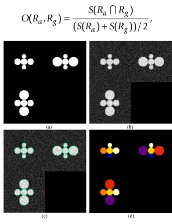
We present an example of the results obtained from apply-ing our proposed nuclei segmentation method on a syn-thesized image. Despite the fact that objects are touching each other and the presence of additive noise, the pro-posed segmentation method has segmented the touching objects perfectly, as shown in Figure 5.

We employ volume overlap measurement methods in order to quantitatively validate our segmentation results. Since there is no ground truth information available for real data and it is very time consuming to manually seg-ment juxtaposed nuclei, instead of using real data, we take advantage of synthesized 3D images. The volume overlap between the automated results and the ground truth is defined as:

O R R S R R

S R S R

a g

a g

a g

( , ) ( )

( ( ) ( ))/ ,

=

+

∩

2

Result on synthesized 3D image segmentation

Figure 5

Result on synthesized 3D image segmentation. (a) The cross-sectional views of binary mask of the synthesized image. (b) The cross-sectional views of synthesized image with added noise. (c) The cross-sectional views of the over-laid boundaries of segmentation on synthesized noisy 3D image. (d) The cross-sectional views of randomly color-coded segmentation result.

(a) (b)

BMC Cell Biology 2007, 8:40 http://www.biomedcentral.com/1471-2121/8/40

where R_a is the automated extracted region and R_g is the ground truth region. The 傽 operator takes the intersection of two regions. S(·) is the volume of the region.

The synthesized 3D touching cell nuclei image is gener-ated as follows: 1) Randomly select a voxel as seed point, and construct a mask of a sphere with a radius 10 mm cen-tered at that point. 2) Generate 6 masks of spheres, which are tangent to the central sphere, with their corresponding radii ranging from 7 mm to 15 mm. This is done to simu-late the variations between radii of real nuclei. 3) Blur the mask images by convolving with a 3D Gaussian kernel, and corrupting it with additive Gaussian noise. For the convenience of visual inspection of the segmentation results, we provide the volume rendering of the original 3D image and surface rendering of the segmentation results. Figure 6a shows the synthesized 3D cell nuclei image, in which the six nuclei are closely touching the central nucleus. The segmentation results with the pro-posed method are illustrated in Figure 6b. Figure 6c shows the segmenation results obtained by global Otsu thresh-olding method. As we can see, the touching objects are not divided correctly in figure 6c.

We have synthesized seven 3D nuclei images. In order to present a quantitative measure for the validation of our results, the average value of volume overlap measurement for the seven cases is around 0.971, and the standard

devi-ation is 0.014. As it is clear from these results, our pro-posed segmentation method achieves significant volume overlap with the ground truth, indicating the accurate per-formance of the gradient flow tracking method.

Validation using 3D C. elegans embryo images

In order to further quantitatively evaluate the segmenta-tion method, we applied the method to C. elegans embryo images. Dr. Sean Megason of California Institute of Tech-nology provided us the C. elegans embryo images. The nuclei are labelled with histone-EGFP. The scope used for the C. elegans image set is a Zeiss LSM510 with a 40X C-Apochromat objective and a 488 nm laser. The original voxel size is 0.14*0.14*0.74 micron in x, y and z direc-tions. In our experiment, the voxel size is re-sampled to isotropic in all directions. The details of the experimental and imaging settings are provided at http://www.digital fish.org/beta/samples/. Two metrics of over-segmentation and under-segmentation were utilized for evaluation of the segmentation method. The over-segmentation metric indicates that a nucleus has been separated into more than one object, or an extracted object has not been labeled as nucleus. This is done in comparison to visual inspection of an expert. The under-segmentation indicates that clusters of nuclei have not been appropriately divided or a nucleus marked by visual inspection was not at all extracted. Four 3D images of C. elegans embryos were used to evaluate the proposed segmentation method based on the above two metrics. Table 1 shows the performance of the proposed segmentation method. On average, the over-segmentation and under-over-segmentation rates are 1.59% and 0.39% respectively, indicating a desirable perform-ance by our segmentation method. The errors are proba-bly caused by the interpolation and re-sampling and inherent noise in the images. For the convenience of vis-ual inspection of the segmentation results, we provide the volume rendering of the original 3D image and surface rendering of the segmentation results. As an example, Fig-ure 7a provides the volume rendering of the original jux-taposed 3D nuclei. The segmentation results represented by surface boundaries are shown in Figure 7b. To validate the segmentation results, two experts manually seg-mented the nuclei respectively, and then we computed the volume overlap between the automated result and that of each of the two experts. We also calculated the volume overlap between the two experts. The mean value of vol-ume overlap is over 95% for both expert 1 and expert 2, and the standard deviation is around 0.02 for both experts, indicating that the automated 3D cell nuclei seg-mentation results are comparable to manual segmenta-tion results.

Validation using 3D zebrafish nuclei images

To further evaluate the proposed segmentation method, we have applied the method to ten 3D zebrafish images in

Illustration of cell nuclei segmentation in 3D space

Figure 4

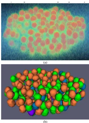
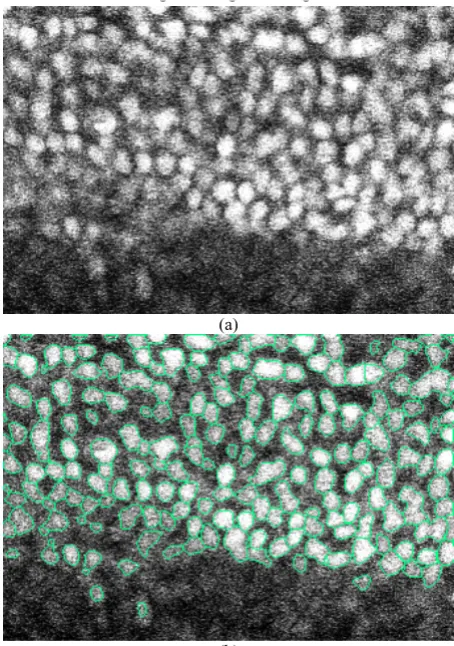
which nuclei are labeled. The 3D zebrafish image datasets are from the Holley Lab at Yale University. These are fluo-rescent confocal images of fixed 12 somite stage zebrafish embryos stained with propidium iodide. All images were collected on a BioRad 1024 confocal microscope using a 25X Zeiss Neofluor objective. For the convenience of vis-ual inspection of the segmentation results, we provide the volume rendering of the original 3D image and surface rendering of the segmentation results. An example of the original 3D image and nuclei segmentation results are shown in Figure 8, in which it is evident that most of the nuclei are segmented correctly, in spite of the fact that many of the nuclei are touching and have irregular shapes. Figure 9 shows a 2D slice of the original image and the segmentation result as shown in Figure 8. The two metrics of over-segmentation and under-segmentation are used to

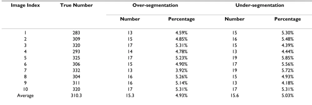
evaluate the segmentation result. Table 2 provides the details of the performance of the segmentation method. On average, there exist 310 cell nuclei for each image, and the over-segmentation and under-segmentation rates are 4.93% and 5.03% respectively. Furthermore, the average volume overlap is over 90% for both expert 1 and expert 2, and the standard deviation is less than 0.02 for both experts, indicating a desirable performance by our seg-mentation method

Discussion

Our method has several advantages over previous approaches. The major advantage of the method is the ability to robustly segment densely packed, touching, or connected nuclei. Additionally, no sophisticated rules are used. The only assumption is that the centers of nuclei are brighter or darker than a nearby region. The fundamental

An example of segmentation result using C

Figure 7

An example of segmentation result using C. elegans embryo image. (a) Volume rendering of original 3D image. (b) Surface rendering of segmentation results. For the con-venience of inspection of touching cell nuclei, the results are randomly color-coded.

p g g g y

(a)

(b) Table 1: The segmentation results of 3D C. elegans embryo images

Image Index True Number Over-segmentation Under-segmentation

Number Percentage Number Percentage

1 187 2 1.07% 0 0.00%

2 187 3 1.60% 1 0.53%

3 185 3 1.62% 0 0.00%

4 192 4 2.08% 2 1.04%

Average 187.75 3 1.59% 0.75 0.39%

Volume and surface rendering of synthesized 3D cell nuclei image and segmentation results

Figure 6

Volume and surface rendering of synthesized 3D cell nuclei image and segmentation results. (a) Volume ren-dering of the synthesized noisy image. (b) Surface renren-dering of the segmentation results with the proposed method, in which each color indicates a segmented object. (c) Surface rendering of the segmentation results with the global Otsu thresholding, in which the touching objects are not divided correctly.

BMC Cell Biology 2007, 8:40 http://www.biomedcentral.com/1471-2121/8/40

difference between our method and existing methods lies in the diffused gradient vector information. In existing methods such as the threshold or watershed methods, intensity is the only adopted information, hence those methods are sensitive to the noise in the image, which usually results in over-segmentation. In contrast, in our method the gradient vector diffusion procedure propa-gates gradient vectors with large magnitudes to the areas with weak gradient vectors and smoothes the noisy gradi-ent vector field. Meanwhile, it preserves the potgradi-ential structural information of the gradient vector field. For example when two nuclei are touching each other, the dif-fused gradient vectors point toward the corresponding centers of the nuclei. This step greatly contributes to the success of touching nuclei segmentation. The disadvan-tage of this method is that it may have difficulty in

processing the images of textured blob objects, since in that situation the gradient vector at the centers of nuclei are cluttered and the condition is violated. Currently the method is implemented using the C/C++ language, with-out using any other common library. Withwith-out any optimi-zation, it takes less than 50 seconds on an Intel Pentium4 2.4 GHz machine with 1 GB memory to segment a vol-ume image with a size of 230*162*80. The running time can be reduced further with multi-resolution implementa-tion and code optimisaimplementa-tion. After evaluating this method on larger and more diverse image datasets, we intend to release the algorithm to the cell biology community.

Conclusion

We presented a novel, automated algorithm for 3D cell nuclei segmentation based on gradient flow tracking. To validate the efficacy and performance of the proposed

seg-2D slice view of the original image and segmentation result in Figure 8

Figure 9

2D slice view of the original image and segmentation result in Figure 8. (a). Original image. (b). The segmented image in which the green curves represent the boundaries of the cell nuclei.

g g g

(a)

(b)

An example of segmentation results of 3D cell nuclei image of zebrafish

Figure 8

An example of segmentation results of 3D cell nuclei image of zebrafish. (a) Volume rendering of original 3D image. (b) Surface rendering of segmentation results. For the convenience of inspection of touching cell nuclei, the results are randomly color-coded.

An example of segmentation results of 3D cell nuclei image of z

(a)

mentation algorithm, we evaluated it by using synthe-sized and real biological images. The results show that the algorithm is able to segment juxtaposed nuclei correctly, a persistent problem in the field of cellular image analysis.

Methods

Gradient vector diffusion by elastic deformation transformation

Gradient information is an important factor in three-dimensional (3D) nuclei segmentation due to the fact that in any given nuclei image, the gradient vectors either point towards the central area of a bright nucleus, or out-wards from the central area of a dark nucleus. However, in practice, the gradient magnitude is very small, and the direction of the gradient vector is usually not trustworthy due to the noise present in the image when approaching the central area of a nucleus. Additionally, when we are dealing with nuclei that are of irregular shapes, the gradi-ent vectors tend to be cluttered. Motivated by these facts, here, we introduce a physical model that incorporates the diffused gradient vectors from the boundaries of the image to generate a smooth gradient field. Our gradient vector diffusion procedure propagates gradient vectors with large magnitudes to the areas with weak gradient vec-tors and smoothes the noisy gradient vector field [11]. For a detailed introduction to gradient vector diffusion, we refer to [11]. We adopt an elastic deformation transforma-tion, under which the image is modeled as elastic sheets warped by an external force field to achieve gradient vec-tor diffusion. This model has been previously employed for image registration [12,13], where the deformation of boundary points are fixed and then the deformation field is propagated to inner regions of the image by solving the elastic model equation. Here, we extend this model to analyze 3D microscopic nuclei images.

The diffused gradient vector field v(x, y, z) = (u(x, y, z), v(x,

y, z), w(x, y, z)) (u(x, y, z), v(x, y, z) and w(x, y, z) are three

components of the diffused gradient vector projecting to

x, y and z axis respectively) in a 3D image is defined to be a solution to the partial differential equation (PDE), also known as a Navier-Stokes equation, describing the defor-mation of an elastic sheet [13]:

µ∇2_{v + (}λ₊ µ₎∇_{div(v) + q × (}∇_{f - v) = 0, (1)}

where ∇2 _{is the Laplacian operator, div is the divergence}

operator, ∇ is the gradient operator, ∇f is the original gra-dient vector field, and Lame's coefficients µand λrefer to the elastic properties of the material. In this paper, we aim to diffuse the gradient vectors toward the central areas of nuclei objects to obtain a gradient flow field. Therefore, f

is set to be

f (x, y, z) = Gσ(x, y, z)*I(x, y, z),

where I(x, y, z) is a 3D intensity image and Gσ(x, y, z) is a

3D Gaussian function with standard derivation σ. Note that before computing the convolution and gradient vec-tor, the images should have been interpolated using a spline-based method and re-sampled to isotropic voxel sizes. q is a function indicating whether or not the dis-placement is pre-fixed at the position. In our method, the indicator function is set as

In our current implementation, the Threshold is set to be 0. Once the Threshold is large, the gradient vectors with small magnitudes will be omitted, including some noisy gradi-ent vectors and some useful gradigradi-ent vectors. Therefore, the Threshold creates a compromise between keeping use-ful gradient vectors and removing noisy gradient vectors. The model is solved by treating u, v and w as functions of time:

q x y z( , , )=_ ∇f x y z( , , ) >Threshold



1

0 otherwise Table 2: The segmentation results of 3D cell nuclei image of zebrafish

Image Index True Number Over-segmentation Under-segmentation

Number Percentage Number Percentage

1 283 13 4.59% 15 5.30%

2 309 15 4.85% 16 5.48%

3 320 17 5.31% 15 4.39%

4 293 14 4.78% 13 4.44%

5 325 17 5.23% 19 5.85%

6 306 15 4.90% 17 5.56%

7 332 13 3.92% 19 5.72%

8 304 16 5.26% 15 4.93%

9 311 16 5.14% 13 4.18%

10 320 17 5.31% 17 5.31%

BMC Cell Biology 2007, 8:40 http://www.biomedcentral.com/1471-2121/8/40

where v_t(x, y, z, t) denotes the partial derivative of v(x, y, z,

t) with respect to time t. The equation is decoupled as:

u_t(x, y, z, t) = µ∇2_{u(x, y, z, t) + (}λ₊ µ_{) (}∇_{div(v(x, y, z, t)))} x

+ q(x, y, z)((∇f(x, y, z))_x - u(x, y, z, t))

v_t (x, y, z, t) = µ∇2_{v(x, y, z, t) + (}λ₊ µ_{) (}∇_{div(v(x, y, z, t)))} y

+ q(x, y, z)((∇f(x, y, z))_y - v(x, y, z, t))

w_t(x, y, z, t) = µ∇2_{w(x, y, z, t) + (}λ₊ µ_{) (}∇_{div(v(x, y, z, t)))} z

+ q(x, y, z)((∇f(x, y, z))z - w(x, y, z, t))

With the finite difference method, by setting the spacing interval ∆x, ∆y, ∆z and time interval ∆t all to be 1 and let-ting the indices i, j, k and n correspond to x, y, z and t

respectively, the equations are approximated as:

The solution to Equation 2 defines the displacement of each position in a 3D elastic object, where displacements at some locations are pre-fixed. In Equation 2, variable v

represents velocity and hence, considering hydromechan-ics rules, the second term in Equation 2 denotes the com-pression level of a compressible fluid. Given this description, setting div(v) = 0 represents an uncompressi-ble fluid. The terms µand λin Equation 2 determine the tradeoff between conformability to the pre-fixed deforma-tion vectors and smoothness of the deformadeforma-tion field [13]. As it is clear from Equation 2, when µ and λ are small, the pre-fixed deformation vectors are preserved. Moreover, having large values for terms µand λwill result in obtaining a smoother deformation field. As an exam-ple, in Figure 1, we demonstrate a comparison between the zoomed diffused gradient vector field with elastic deformation transformation and the original gradient vec-tor field of a slice from a 3D nucleus image. As is clear from Figure 1, the diffused vector field using the elastic deformable model flows more smoothly towards the cen-tral areas of nuclei compared to the original gradient

vec-tor field. Moreover, even though nuclei are closely juxtaposed, the diffused flow field splits along a clear boundary and flows towards the corresponding central areas of each nucleus. This property greatly contributes to the success of 3D nucleus segmentation.

Gradient flow tracking

In the diffused gradient vector field, the vectors flow toward the sinks, which correspond to the centers of nuclei. To follow the vectors until they stop at the sinks, the gradient flow tracking procedure is performed as fol-lows. From any starting point x = (x, y, z), the next point

x' = (x', y', z') that x flows through in the diffused gradient field is computed as:

vt( , , , )x y z t = ∇µ 2v( , , , ) (x y z t +λ µ+ ∇) div( ( , , , ))vx y z t +q x y z( , , )(∇ff x y z x y z t x y z f x y z

( , , ) ( , , , )) ( , , , ) ( , , ) − = ∇     v v 0 (2)

u_t =un_{i j k, ,}+1−u_{i j k}n_{, ,} , v_t=vn_{i j k, ,}+1−v_{i j k}n_{, ,} , w_t=w_{i j k}n_{, ,}+1−w_in_{,jj k}

i j k i j k i j k i j k i j k i

u u u u u u u

,

, , , , , , , , , , ,

,

∇2 = +1 + −1 + +1 + −1 + +1+ jj k i j k

i j k i j k i j k i j k i j

u

v v v v v v

, , , , , , , , , , , , − + − + − − ∇ = + + + + 1 2

1 1 1 1

6

,, , , , ,

, , , , , , ,

k i j k i j k

i j k i j k i j k i j

v v

w w w w w

+ − + − + − + − ∇ = + + + 1 1 2

1 1 1

6

1

1 1 1

1 1

6

, , , , , , ,

, , , ,

( ( ))

k i j k i j k i j k

x i j k i j k

w w w

div u u

+ + −

∇ = +

+ −

+ −

v −− + − − +

+ −

+ + + +

+ +

2 1 1 1 1

1 1

u v v v v

w w

i j k i j k i j k i j k i j k

i j k

, , , , , , , , , ,

, , ii j k i j k i j k

y i j k i j k i j

w w div v v v

, , , , , , , , , , , ( ( )) + + + − − + ∇ = + − 1 1

1 1 2

v ,, , , , , , , , ,

, , , ,

k i j k i j k i j k i j k

i j k i j k

u u u u

w w

+ − − +

+ −

+ + + +

+ + +

1 1 1 1

1 1 11 1

1 1 2

− +

∇ = + − +

+

+ − +

w w

div w w w u

i j k i j k

z i j k i j k i j k i

, , , ,

, , , , , ,

( ( ))v 11 1 1 1

1 1 1

, , , , , , , ,

, , , , ,

j k i j k i j k i j k

i j k i j k i j

u u u

v v v

+ + + + + + − − + + − − ++ + + + ∇ = − ∇ = − ∇ 1 1 1 , , , , , , , , , , , ( ) , ( ) , (

k i j k

x i j k i j k y i j k i j k

v

f f f f f f ff)_z =f_{i j k, ,+1}−f_{i j k, ,}

The 3D view of gradient vector field and diffused gradient vector field with elastic deformation transformation of a slice cropped from a 3D cell nuclei image

Figure 1

The 3D view of gradient vector field and diffused gra-dient vector field with elastic deformation transfor-mation of a slice cropped from a 3D cell nuclei image. (a). A slice of the 3D image. (b). The original gradient vector field. (c). The diffused gradient flow field with elastic defor-mation transfordefor-mation. Obviously, the diffused vector field with elastic deformation transformation smoothly flows toward the central areas of cell nuclei. (d). Zoomed view of (b). (e). Zoomed view of (c).

g

Here, v(x) is the diffused gradient vector at point x, and "round" returns the nearest integer. The angle between the diffused gradient vectors of these two adjacent points is determined as:

When the angle between two consecutive diffused gradi-ent vectors is less than 90 degrees, the gradigradi-ent flow track-ing procedure continues. Otherwise, the gradient flow tracking procedure is stopped, and a sink is reached. In this way, the vectors at each point along the tracking curve define a smooth path leading to a sink. In practice, seg-mentation of images into nuclei can be obtained by start-ing a gradient flow trackstart-ing procedure from every point in image. The set of pixels that flow to the same sink natu-rally produce the attraction basin of the sink. All points in the same attraction basin are segmented as an object (nucleus). All points are tracked independently, thus the attraction basin can be of arbitrary shape. After the gradi-ent flow tracking step if the sinks are very close to each

other, the attraction basins of the sink are combined together to obtain a larger attraction basin. In all our experiments, if the distance between two sinks is less than three pixels the attraction basins of the two sinks are com-bined together to obtain a larger attraction basin. Figure 2 shows an illustration of the result of the gradient flow tracking based method.

The algorithm of the gradient flow tracking is summarized as follows.

1. Randomly select a point x as the initial point x0_.

2. Obtain xn + 1 _{(n = 0,1,2...) using Equation 3 based on x}n_.

3. Compute the angle θ_n of diffused gradient vector between xn + 1 _{and x}n _{with Equation 4. If} θ

n is larger than

, stop.

4. Replace xn _{with x}n + 1_{. Return to step 2.}

Gradient flow tracking is applied to each point in the image. All points in the same attraction basin are grouped into the same cluster. Since it is time consuming to run the tracking algorithm for every point, in order to improve the performance of our method, gradient flow tracking is not applied to the points that have already been on the gradi-ent flow trajectory of a previously processed pixel. Instead, these visited points are directly associated with the sink to which the path flows. This improvement not only speeds up the segmentation, but also yields reproducible seg-mentation results.

Local adaptive thresholding

After the gradient flow tracking step, the image is seg-mented into smaller regions each of which is expected to contain only a single nucleus. From here the nuclei seg-mentation problem is turned into binary classification problem where we are interested in distinguishing the nuclei from their background in a small region. Therefore an intensity thresholding method is appropriate for extracting the nuclei from the background. In order to approach this problem, we can take advantage of the method employed by Otsu in [14], which has the ability to extract the nucleus from each attraction basin. Another approach for dealing with this problem is through design-ing a more involved method that employs techniques such as graph cut, level set, etc. Here, we employ the locally adaptive method of Otsu [14] because of its ability to deal with situations where the intensity of nuclei and background are not constant across an image. In each seg-mented region, pixels whose intensities are larger than the automatically determined local Otsu threshold are ′ = + 



 _

x x v x

v x round ( )

( ) (3)

θ = ′

′

arccos ( )

( ) , ( ) ( ) v x

v x v x

v x (4)

π

2

Illustration of the gradient flow tracking based segmentation method

Figure 2

Illustration of the gradient flow tracking based seg-mentation method. (a). Clustered gradient vectors in 3D space. (b). Zoomed view of selected clusters of gradient vec-tors. Each color represents a separated cell.

(a)

BMC Cell Biology 2007, 8:40 http://www.biomedcentral.com/1471-2121/8/40

grouped as nuclei, otherwise they are grouped as back-ground. Finally, an optional procedure is performed after extracting the nuclei to eliminate small regions, which contain a lower number of pixels than a threshold.

Summary of 3D cell nuclei segmentation method

The algorithm of the 3D cell nuclei segmentation method based on gradient flow tracking is summarized as follows.

1. Obtain the diffuse gradient vector field using the elastic deformation transformation

2. From each point, run the gradient flow tracking proce-dure, and label each passed pixel with a converged sink position.

3. Combine the attraction basins of the sinks whose dis-tance is less than three pixels.

4. Assign the same label to the points in the same attrac-tion basin.

5. Perform local adaptive thresholding in each attraction basin to extract the nucleus.

6. Optional procedure: eliminate regions with smaller number of pixels than a threshold T.

Running example

Figure 3 provides an illustration of 3D nuclei segmenta-tion on a 2D slice. In Figure 3b, we demonstrate the initial subdivision of the image into nuclei areas after the gradi-ent flow tracking procedure. As it is clear from these images, each nucleus is enclosed by a boundary. The nuclei segmentation results after the adaptive threshold-ing is provided in Figure 3c, and their randomly color-coded representation is shown in Figure 3d.

Figure 4 provides an illustration of the 3D nuclei segmen-tation procedure in the 3D space. In Figure 4a, the cross-sectional views of a 3D image are shown. Figure 4b renders the boundary surfaces of extracted 3D nuclei. For the convenience of inspection of touching nuclei, the extracted nuclei are randomly color-coded.

Authors' contributions

GL and TL proposed the algorithm. GL implemented the algorithm. JN helped implement the algorithm. AT and STCW verified the algorithm and the result. AM and SH acquired the image data and provided biological input to this work.

Additional material

Additional file 1

The computer program, called CellSegmentation3D, loads the 3D Ana-lyze format image (the suffix ".img" or ".hdr" is not needed in the input image name), and the segmentation result is also saved as the Analyze for-mat. For each 3D input image, the program will output two results: 1) the segmentation result, in which all voxels belonging to the same cell are labelled with the same unique intensity; 2) the boundary map that sepa-rates segmented cells. Usage: CellSegmentation3D image_Input -f fusion_threshold -m min_Region -d diffusion_iteration -s sigma; Default parameters: fusion_threshold 3, min_Region 50, diffusion_iteration 15, sigma 1.0; For example: CellSegmentation3D elegans-01-01 -f 3 -m 35. This will produce the two result images: elegans-01-01_edge.img and

elegans-01-01_segmentation.img. Notes that the segmentation results can be inspected by many visualization tools, provided that they can load 3D Analyze format images. The NIH ImageJ progam (freely downloada-ble at: http://rsb.info.nih.gov/ij/) is recommended.

Click here for file

[http://www.biomedcentral.com/content/supplementary/1471-2121-8-40-S1.exe]

Additional file 2

The elegans-01-01.img is an example image file.

Click here for file

[http://www.biomedcentral.com/content/supplementary/1471-2121-8-40-S2.img]

Illustration of 3D cell nuclei segmentation on a 2D slice

Figure 3

Illustration of 3D cell nuclei segmentation on a 2D slice. (a) A slice from 3D cell nuclei image. (b)Boundaries of small regions overlaid on the slice. The boundaries are obtained by the method in Section 2.2. (c) Edges of cell nuclei overlaid on the slice after the step of adaptive thresholding in Section 2.3. (d) Randomly color-coded extracted cells.

(a) (b)

Publish with BioMed Central and every scientist can read your work free of charge "BioMed Central will be the most significant development for disseminating the results of biomedical researc h in our lifetime."

Sir Paul Nurse, Cancer Research UK

Your research papers will be:

available free of charge to the entire biomedical community

peer reviewed and published immediately upon acceptance

cited in PubMed and archived on PubMed Central

yours — you keep the copyright

Submit your manuscript here:

http://www.biomedcentral.com/info/publishing_adv.asp

BioMedcentral

Acknowledgements

This work is funded by a Bioinformatics Research Center Program Grant from Harvard Center for Neurodegeneration and Repair, Harvard Medical School (STCW). We would like to thank Dr. Sean Megason of California Institute of Technology for providing the C. elegans embryo images.

References

1. Holley SA, Geisler R, Nüsslein-Volhard C: Control of her1 expres-sion during zebrafish somitogenesis by a Delta-dependent oscillator and an independent wavefront activity. Genes & Dev

2000, 14:1678-1690.

2. Jülich D, Hwee LC, Round J, Nicoliaje C, Scroeder J, Davies A, Geisler R, Lewis J, Jiang YJ, Holley SA: beamter/deltaC and the role of Notch ligands in the zebrafish somite segmentation, hind-brain neurogenesis and hypochord differentiation. Dev Biol

2005, 286:391-404.

3. Lin G, Adiga U, Olson K, Guzowski J, Barnes C, Roysam B: A hybrid 3-D watershed algorithm incorporating gradient cues and object models for automatic segmentation of nuclei in con-focal image stacks. Cytometry 2003, 56A:23-36.

4. Lin G, Chawla MK, Olson K, Guzowski JF, Barnes CA, Roysam B:

Hierarchical, model-based merging of multiple fragments for improvoed three-dimensional segmentation of nuclei.

Cytometry 2005, 63A:20-33.

5. Umesh Adiga PS, Chaudhuri BB: An efficient method based on watershed and rule-based merging for segmentation of 3-D histo-pathological images. Pattern Recognition 2001,

34:1449-1458.

6. Belien JAM, Ginkel HAHM, Tekola P, Ploeger LS, Poulin NM, Baak JPA, Diest PJ: Confocal DNA Cytometry: A Contour-Based Segmentation Algorithm for Automated Three-Dimen-sional Image Segmentation. Cytometry 2002, 49:12-21. 7. Wahlby C, Sintorn IM, Erlandsson F, Borgefors G, Bengtsson E:

Com-bining intensity, edge and shape information for 2D and 3D segmentation of cell nuclei in tissue sections. J Microsc 2004,

215:67-76.

8. Dufour A, Shinin V, Tajbakhsh S, Guillen-Aghion N, Olivo-Marin JC, Zimmer C: Segmentation and Tracking Fluorescent Cells in Dynamic 3-D Microscopy with Coupled Active Surfaces. IEEE Trans Image Processing 2005, 14:1396-1410.

9. Sarti A, de Solorzano CO, Locket S, Malladi R: A Geometric Model for 3-D Confocal Image Analysis. IEEE Trans Biomedical Engineer-ing 2000, 47:1600-1609.

10. Vincent L, Soille P: Watersheds in digital spaces: an efficient algorithm based on immersion simulations. IEEE Trans Pattern Anal Mach Intell 1991, 13:583-598.

11. Xu C, Prince J: Snakes, shapes, and gradient vector flow. IEEE Trans Image Processing 1998, 7:359-369.

12. Bajcsy R, Kovacic S: Multiresolution elastic matching. Computer Vision, Graphics and Image Processing 1989, 46:1-21.

13. Davatzikos C, Prince J, Bryan R: Image Registration Based on Boundary Mapping. IEEE Trans Med Imaging 1996, 15:112-115. 14. Otsu N: A threshold selection method from gray-level

histo-grams. IEEE Trans Systems Man Cybernetics 1979, 9:62-66. 15. Ortiz de Solorzano C, Garcia Rodriguez E, Jones A, Pinkel D, Gray

JW, Sudar D, Lockett SJ: Segmentation of confocal microscope images of cell nuclei in thick tissue sections. J Microsc 1999,

193(Pt 3):212-26.

16. De Solorzano CO, Malladi R, Lelievre SA, Lockett SJ: Segmentation of nuclei and cells using membrane related protein markers.

J Microsc 2001, 201(Pt 3):404-415.

Additional file 3

The elegans-01-01.hdr is the header file associated with the image.

Click here for file