3973
RTDBSTREAM: A REAL-TIME DENSITY-BASED
CLUSTERING FOR EVOLVING DATA STREAMS
1K. SHYAM SUNDER REDDY, 2C. SHOBA BINDU
1Research Scholar, JNTUA, Ananthapuramu, INDIA
2Department of CSE, JNTU College of Engineering, Ananthapuramu, INDIA
E-mail: [email protected], 2[email protected]
ABSTRACT
Density-based clustering method has come into existence as a prominent class for clustering data streams. It has the ability to discover clusters with arbitrary shape, and it can handle noise in data. Recently, several density-based clustering algorithms have been proposed in the literature for clustering data streams. But each algorithm has its own limitation that renders them ineffective and makes a new algorithm necessary for dealing with big data. Existing density-based clustering algorithms require high computation time and more memory for clustering process. In this paper, we present a novel density-based clustering algorithm called Real-time Density-based Clustering (RTDBStream) for evolving data streams. This algorithm is a hybrid density-based clustering algorithm that integrates the pros of density-grid and density micro-clustering algorithms to get better results. The quality of the proposed algorithm is evaluated on various data sets with distinct characteristics using different quality metrics.
Keywords: Big data, Data stream, Density-based clustering, Grid-based clustering, Micro-clustering
1. INTRODUCTION
The amount of data being produced by real-time applications has significantly increased over the past few years. Advancement in technology and innovation in various sectors has given rise to increase in data. The growing field of applications such as healthcare, banking, agriculture, weather monitoring, stock trading, education, medicine, science and other sectors has led to the creation of large amounts of data, often known as big data [1]. Every day a huge amount of data is being produced continuously as data streams from different real-time applications. Data streams are evolving over time, and the amount of data is unbounded [2]. Hence it is not possible to keep the whole data stream in the main memory. The main problem associated with these data streams are their management, storage, analysis, and retrieval. Users are interested in gaining the knowledge out of these data streams during their same minute of generation. However, management of big data is not an easy process; the intricacies that lie within the management of big data do not support the use of conventional technologies and methods [3].
Traditional methods of handling data involve the use of techniques which hold limited capabilities, inelastic and their storage capacities do not support handling of a large amount of data. Conventional clustering algorithms require data to be scanned a
number of times before it can detect and process the clusters of data. This strategy is inefficient when it comes to big data, because the scale of the data prohibits it from being scanned over and over again. Big data is differentiated from traditional data processing systems in the dimensions such as speed of decision making, complexity processing, structured and unstructured data processing, the flexibility of processing data, and concurrency [4]. While traditional clustering algorithms are applicable only to static data, today’s research issues and applications in big data have to deal with infinite, continuous streams of data, arriving at high speed.
One of the ways of dealing with such a huge amount of data is to classify it into sets of meaningful categories. This is where clustering comes into the picture. Clustering is a well-established data mining technique that aims at grouping data objects into clusters C={C1, C2, C3 ... Ck} such that similar data
objects are assigned to the same cluster while dissimilar data objects are assigned to different clusters.
3974 evolving data, handling high-dimensional data, and single pass clustering [2]. In data stream clustering discovering arbitrary shape clusters and detecting noise is very important.
2. RELATED WORK
Clustering can be classified into different categories based on different criteria: Hierarchical clustering, Grid-based clustering, Partitioning clustering, Model-based clustering and Density-based clustering [5]. Among all the clustering algorithms density-based clustering methods are more appropriate in data streams clustering. This is because density-based clustering is designed with an ability to discover clusters that have arbitrary shapes and able to make noise/outliers detection. Other clustering algorithms require the knowledge of the number of clusters once the clustering process begins. However, density-based clustering algorithms are independent of the cluster numbers and hence have no assumption on the number prior to the process.
The density-based clustering is developed and designed on the basis of the notion of density. The clusters are prepared in a dense area using a density function. The primary notions constantly add until the density of the neighbourhood cluster crossed to some extent or limit. The method can be used to filter out the outliers/noise and locates the cluster at various arbitrary shapes. DBSCAN [6], NBC [7] OPTICS [8], and DENCLUE [9] are examples of some of the primary algorithms that are based on density.
DBSCAN [6] (Density-Based Spatial Clustering of Applications with Noise) refers to a high quality scalable density-based clustering method that depends on the notion of the density of clusters. The two essential user-specified input parameters for DBSCAN are Eps and µ, where Eps
is the maximum radius of the neighbourhood and µ
is the minimum number of points in the Eps -neighbourhood of a point. DBSCAN starts the clustering process by randomly selecting a point p
and checks the condition whether NEps(p) contains at
least µ number of points. If the condition is satisfied, then the point p is considered as a core point, and a new cluster is formed. Otherwise, the point p is considered as a noise point. Arbitrary shaped clusters along with noise/outlier can be found using DBSCAN algorithm. However, the application of DBSCAN to high dimensional features are failed to investigate, and it fails to detect the clusters with multi-density.
The NBC [7] (Neighbourhood-Based Clustering) clustering algorithm also belongs to the class of density-based clustering algorithms. NBC algorithm can discover arbitrary shape clusters, and it requires fewer input parameters than the existing algorithms. NBC algorithm can cluster high-dimensional data sets efficiently. OPTICS [8] (Ordering Points to Identify the Clustering Structure) extends DBSCAN in order to cluster data points from a range of parameter settings. OPTICS algorithm differentiates considerable objects from outliers or noise thereby identifying all cluster levels in a data set. DENCLUE [9] is a clustering algorithm that applies the kernel density estimation to employ a cluster model, and clusters the object found on the set of density distribution function. The algorithm uses the idea of density attracted regions to form clusters. However, the algorithm is not suitable for data sets of high dimension.
There is a wide range of algorithms in the literature for clustering the static data sets inwhich few have been extended their application towards the data streams. In the clustering process, all these algorithms uses density-based methods and overcome the challenging issues, which are put out by data streams nature. The existing density-based algorithms for clustering data streams are categorized into two broad groups: 1) Density-based micro-clustering algorithms and 2) Density-grid based clustering algorithms.
2.1 Density-Based Micro-Clustering Algorithms
Micro-clustering is one of the most important methods in data stream clustering to compress data streams efficiently. The concept of micro-cluster (µC) was first proposed by Zhang et al. in [10]. It is an extension of Cluster Feature Vector (CFV) which is a triple summarizing the information maintained about the cluster. Density-based micro-clustering algorithms uses µCs to keep summary information about data streams and clustering is performed on these µCs.
Cao et al. In [11] proposed a density-based
3975 In [12], Tasoulis et al. proposed an algorithm termed as OpticsStream that uses µC concept for clustering data streams. OpticsStream is an extension of OPTICS [8] algorithm in which data stream cluster structures are represented graphically. It has the ability to handle noisy and evolving data.
OpticsStream cannot handle high-dimensional data.
Menasalvas et al. In [13] proposed a
density-based micro-clustering algorithm termed as
C-DenStream in which constraints are applied for data
stream clustering. It adds the constraints to the µCs
by including the domain information in the form of constraints. C-DenStream has the ability to discover arbitrary shape clusters with constraints. However, this algorithm has high computation time, and it cannot handle high-dimensional data.
In [14], Jink et al. proposed a three-step density-based clustering algorithm termed as
rDenStream for clustering data streams. The
algorithm is based on DenStream with an additional step called retrospect. In the retrospect phase, the misinterpreted abandoned data points get a new chance to be re-learned and to enhance the strength of the clustering. It improves the accuracy of the clustering algorithm by creating a classifier from the clustering result. However, the time complexity and memory usage of rDenStream is high since it processes and retains the old buffer.
Ren et al. In [15] proposed an algorithm termed
as SDStream for clustering data streams over a
sliding window. SDStream is an online-offline phase clustering algorithm that processes most recent data, and summarizes the old data by using sliding window model. The algorithm considers the most recent data stream distribution, and it discards the data points which are not accommodated in a sliding window length. SDStream has the ability to handle noisy and evolving data, and it cannot handle high-dimensional data.
In [16], Lin et al. proposed an online-offline clustering algorithm termed as HDenStream for evolving heterogeneous data streams. The pruning phase of HDenStream is similar to that of
DenStream. The algorithm can cover continuous and
categorical data, which makes it more useful since we have any kind of data in the real world applications. However, the algorithm cannot handle high-dimensional data.
Dunham et al. In [17] proposed a density-based
algorithm termed as SOStream (Self Organizing density-based clustering over data Stream) that has the only online phase in which it dynamically creates, merges, and removes clusters. SOStream
uses competitive learning where a winner influences its immediate neighbourhood. SOStream
automatically adapts the threshold value for density-based clustering, and it detects clusters within fast evolving data streams. SOStream has high computation time and it cannot handle high-dimensional data.
In [18], Zimek et al. proposed an online-offline phase clustering algorithm termed as HDDStream
for clustering high dimensional data streams. The online phase maintains the summary of both points and dimensions. The final clusters are discovered in offline phase based on a PreDeConStream[19] clustering algorithm. HDDStream has the ability to handle evolving data streams and noisy data. However, it cannot process the data in a limited time.
Spaus et al. In [19] proposed a clustering
algorithm termed as PreDeConStream which is similar to HDDStream. By working in the offline phase, PreDeConStream improves the efficiency of
the HDDStream. The algorithm can cluster
high-dimensional data. It introduces a subspace prefer vector and it maintains two lists including outlier and potential µC. However, the algorithm takes more time for searching the affected neighboring clusters. In [20], Pizzuti et al. proposed an algorithm based on a bio-inspired model (flocking model). The algorithm is termed as FlockStream which is more efficient than DenStream since the number of comparisons is limited. This method is based on a flocking model in which agents (µCs) work independently but form clusters together.
FlockStream cannot handle high-dimensional data.
2.2 Density Grid-Based Clustering Algorithms
3976 landmark window model, sliding window model and fading window model for handling evolving data.
Li et al. In [21] proposed an incremental one
pass density grid-based clustering algorithm termed
as DUCStream (Dense Units Clustering for Data
Stream) for data streams using the dense unit. When a dense unit is added, a new cluster is created only if there is no related cluster; otherwise, the new dense unit is consumed to the existing clusters.
DUCStream utilizes bitwise clustering. The
algorithm has the ability to handle noisy data, and it has less time and space complexity. However, the algorithm cannot handle evolving data.
In [22], Chen et al. proposed an online-offline algorithm termed as DStream-I for clustering real-time stream data. The online phase updates the characteristic vector of the grid by reading a new data point and maps it into the grid. In the offline phase, clusters are adjusted in each time interval gap and update the grid density and then perform the clustering. DStream-I cannot handle high-dimensional data since it assumes that the maximum grids are empty in the high-dimensional locality.
Tan et al. In [23] proposed an online-offline
algorithm termed as DDStream that improves the quality of the cluster by detecting the border points in the grids. In online phase, the characteristic vector of the grid is updated. In each time interval gap, the offline phase runs and extracts the boundary points, and clusters the dense grids. DDStream cannot handle high-dimensional data and it has high time complexity.
In [24], Chen et al. proposed an algorithm termed as DStream-II that is based on the density of the grid attraction. Grid attraction presents that to what extent the data in one neighbor is adjoining to that of another neighbor. It has pruning techniques to remove the sporadic grids mapped by the outliers and to adjust the clusters in each time interval gap.
DStream-II improves the cluster quality by
considering the position of the data in the grids for clustering. However, how to remove sporadic grids is an open issue in DStream-II. It cannot handle high-dimensional data.
Wan et al. In [25] proposed an online-offline
algorithm for clustering data streams at multiple resolutions, called as MR-Stream. In the online phase, the algorithm enables the new data point to be mapped to its related grid cell. The offline phase discovers clusters at a user-defined height. In
MR-Stream, a memory sampling method is introduced to
run the offline component. It improves the performance by running the offline component at constant times. However, the algorithm cannot handle high-dimensional data.
In [26], Ren et al. proposed an online-offline algorithm termed as PKS-Stream that uses PKS-tree for recording non-empty grids and their relations. The algorithm uses k-cover grid cells for maintaining non-empty cells. In online phase, the data records are mapped to the related grid cells; otherwise, a new grid cell is created if there is no grid cell for the data record. In offline phase, the clusters are formed based on the dense neighboring grids.
PKS-Stream has the ability to handle
high-dimensional data streams. However, it cannot handle the issues like limited time and limited memory.
Yang et al. In [27] proposed a clustering
algorithm termed as DCUStream for uncertain data. For each object in the stream, a tuple that maintains data point, existence probability of the data point, and its time of arrival are considered. It has the ability to handle noisy and evolving data. However, the clustering process is time-consuming since it searches the core dense grids and finds their neighbors.
In [28], Amineh et al. proposed a clustering algorithm termed as DENGRIS-Stream over a sliding window. It maps each data point into a grid, computes each grid density, and clusters the grids using density methods. DENGRIS-Stream is the first density clustering algorithm for evolving data streams over sliding window model.
Kaur et al. In [29] proposed an online-offline
algorithm for heterogeneous data streams termed as
ExCC (Exclusive and Complete Clustering). Online phase maintains synopsis in the grids and the final clusters are formed on demand in the offline phase.
ExCC can cover data stream with numeric and categorical attributes. It cannot handle high-dimensional data. It requires more memory to store and more time to process.
From the literature, we observed that the existing density-based clustering algorithms require high computation time and more memory for clustering evolving data streams. In this paper, we propose a novel hybrid density-based clustering algorithm for evolving data streams.
3. PROPOSED METHOD
In out proposed method, we use a fading (damped) window model to capture the data streams. In data stream clustering, aging is an important concept. High level of importance will be given to more recent data by assigning a weight for every point via a fading (aging) function. The fading function is defined as f(t)= 2-λt where f is a fading
3977 data of the streams. According to this fading function, the weight of the data stream point’s decreases exponentially with time t. The larger the value of λ, the lower importance is given to historical (old) data.
3.1 Basic Concepts and Definitions
Definition 1. Data Stream: A data stream (DS) is an
infinite sequence of ordered data objects p1, p2 ... pi
arriving at time stamps t1, t2 ... ti, that can be read
once using limited processing and storage capabilities. This sequence of data objects can be endless and usually flows at high speed.
Definition 2. Weight of a Data point (wp): For each
data point p in the data stream, we assign it a density
coefficient which decreases over time t (as p ages).
The initial weight of the data point is 1. Let tp be the
arrival time of a data point p. The weight of a data point p at current timestamp tc where tc>tp is defined
as follows:
wp(tc) = wp(tp) . f(tc-tp) = 2
Where wp(tp) is the weight of the data point p at
time tp.
Definition 3. Grid density (wg): Weight (density) of
a grid g at current timestamp tc is defined as follows:
wg(tc)= ∑ ∈ 2
Grid weight wg is based on the sum of weights of
data points that are mapped to grid g. The weight of any grid is constantly changing. However, it is unnecessary to update the weights of all data points and grids at every time stamp. Instead, we update the weight of a grid only when a new data point is mapped to the grid. The grid weight is updated at current timestamp tc with the last updated timestamp
tg as follows [22]:
wg(tc) = wg(tg) * f(tc-tg) + 1
The sum of weights of all the data points has an upper bound of , and the average density of each grid is where Ng is the number of
grids.
Definition 4. Core point: A core point is defined as
an object in whose ε-neighbourhood, the overall weight of the data points is at least an integer µ.
Definition 5. Density area: Union of
ε-neighbourhoods of core points is defined as density area.
Definition 6. Dense grid: For a grid g, at timestamp
t, if wg(t)≥ , where β > 0 is a controlling
threshold, then we call it as a dense grid.
Definition 7. Sparse grid: For a grid g, at timestamp
t, we call it a sparse grid if wg(t) < .
Definition 8. Core-micro-cluster (cµC): A core µC
at time t is defined as cµC(w, c, r) for a group of close data points , … with time stamps
, … as follows:
1. Weight, w=∑ , w ≥µ
2. Center, c=∑
3. Radius, r=∑ , with r≤ε, where
, c denotes the Euclidean distance between the center c and data point . Where µ represents the minimum number of weighted points needed to be within the NEps(c) in
order to make the current micro-cluster a core µC.
Definition 9. Maximum weight of cµC: If all the
data points of the data stream are inserted into the
same µC, then wcµC=∑ t =
∑ 2 can be transformed with the sum formula for geometric series as follows:
∑ 2 .
Thus the maximum weight of any µC is: wcµC = lim
→ = .
Notice that the weight of cµC must be above or equal to µ, and the radius must be below or equal to ε.
Definition 10. Potential micro-cluster (pµC): A
potential µC at time t is defined as pµC(w,
, , c, r) for a group of close data points
, … with time stamps , … as follows:
1. Weight, w=∑ , w ≥βµ, where β,
0<β<1, is the parameter to determine the threshold of an outlier relative to cµCs.
2. Weighted linear sum of the points, =
∑
3. Weighted squared sum of the points, =
∑
4. Center of pµC, c=
5. Radius ofpµC, r= | | | | with r≤ε.
Definition 11. Directly density-reachable: A pµC cp
is directly density-reachable from a pµC cq with
respect to µ and ε, if the weight of cq is greater than
µ and dist(cp, cq)<rp+rq.
Definition 12. Density-reachable: A pµC cp is
density-reachable from a pµC cq with respect to µ
and ε, if there is a chain of micro-clusters , … ,
such that , and , such that is
directly density-reachable from , with respect to
3978
Definition 13. Density-connected: A pµC cp is
density-connected from a pµC cq with respect to ε
and µ, if there is a p-micro cluster ck such that both
cp and cq are density-reachable from ck with respect
to µ and ε.
Definition 14. Grid Characteristic Vector (CV):
Characteristic vector is a tuple CV(ng, tg, wg) where
ng is the number of data points, tg is the last updated
timestamp and wg is the grid weight.
Definition 15. Density threshold function (Δ):
Density threshold function [22] is considered for the sporadic grids which do not receive any data points for long time. In fact, sporadic grids do not have any chance to be converted to dense grids and consequently to pµC. If wg<Δ, then we can safely
delete the grid from the grid list (in the outlier buffer). If the last update time of a grid g is tg, then,
at current time tc, (tc>tg), the density threshold
function is defined as follows [32]:
Δ(tc,tg)= ∑ 2 =
Definition 16. Pruning time: For each existing pµC
cp, if no new data point is added to it, the weight of
cp will decay gradually. If the weight is less than βµ,
then cp becomes an outlier, and it should be deleted
from the memory. We check the weights of all µCs
as well as the weights of all grid cells in a time we call tr. Time tr is the minimum time for a pµC in
timestamp t1 to be converted to an outlier in t2 (t2>t1)
which is described as follows: tr = log
Proof:
w(t2) = w(t1) * f(t2-t1) +1
w(t2)= w(t1) * 2 +1,
βµ= βµ * 2 + 1, tr= t2-t1,
βµ= βµ * 2 . + 1 tr = log
3.2 RTDBStream Algorithm
RTDBStream is an online-offline clustering algorithm for evolving data streams. It is a hybrid density-based clustering algorithm that integrates the pros of density-grid and density micro-clustering algorithms. The online component of RTDBStream has two phases: Initialization phase and the Pruning
phase. In the online phase, RTDBStream
continuously reads a data point from the data stream and adds it to an existing µC or maps it to the grid. The online phase keeps the summary statistics of the data streams in the form of pµC’s. In the offline phase (Reclustering phase), RTDBStream generates the final clusters on demand by the user by applying
3979 Working of the RTDBStream algorithm is divided into three phases as follows:
Initialization phase: In the initialization phase, the
minimum timestamp tr is computed based on user’s
parameter settings. Furthermore, the new data point
p is merged to an existing µC or mapped to the grid. The procedure is as follows:
1. When a new data point p arrives, RTDBStream finds the nearest pµCcp to the point p and then
we try to merge p into cp.
2. If rp, the new radius of cp , is less than or equal
to ε, then point p will be inserted into cp.
3. Else, the data point p is mapped into the grid g
in the outlier buffer.
4. If the total number of data points in the grid g
reaches µ, then we check the grid density. 5. If the grid weight wg is greater than the dense
grid threshold, then we form a new pµC, out of the data points in the grid g
6. The related grid g of the new pµC is deleted from the grid list.
Algorithm 2: Pruning ( )
1) for all grid g in grid_listdo
2) Δ(tc,tg)=
;
3) //detecting and removing sporadic grids 4) if wg<Δthen
5) delete grid g from the grid_list;
6) end if 7) end for
8) for eachpµC in pµC_list do 9) //detecting and removing outlier µCs
10) if w < β.µ then
11) delete pµC from pµC_list; 12) end if
13) end for
Pruning phase: The procedure of pruning phase is
shown in Algorithm 2. In this phase, sporadic grids and the outlier µCs are removed. The weights of grids and pµCs are checked periodically at pruning time tr. For each existing pµC cp, if no new data point
is added to it, the weight of cp will decay gradually.
Furthermore, there are few grids which do not receive any data points for a long time and become sporadic. The grids and the µCs with the weights less than a threshold are removed from the grid list and
pµC list, respectively, and the memory space is released.
Clustering phase: The online phase maintains pµCs
that capture the density area of data streams. However, in order to generate meaningful clusters, it is necessary to apply some clustering algorithm to get the final result. In this phase, the final clusters are
formed from pµCs by using a variant of DBSCAN. Each micro-cluster pµC is considered as a virtual point located at the center of pµC with the weight w. In order to determine the final clusters, we adopt the density-connectivity concept of DBSCAN algorithm [6]. The variant of DBSCAN algorithm consists of two parameters: ε and µ.
4. EXPERIMENTAL RESULTS
We now present the experimental evaluation of RTDBStream with respect to two existing clustering algorithms namely, DenStream and D-Stream. RTDBStream as well as the comparative methods were implemented in Java in the MOA framework [30]. All the experiments were conducted on an Intel(R) core(TM) i5-2.5GHz processor with 8GB RAM, running Microsoft Windows XP. To evaluate the RTDBStream, both synthetic and real data sets were used. The parameters for RTDBStream algorithm were set as follows: initial number of points initPoints= 1000, decay factor λ=0.5, outlier threshold β=0.5, µ=10, and ε=15.
4.1 Data sets and Evaluation
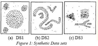
[image:7.612.315.520.505.602.2]We have used three synthetic data sets, DS1, DS2, and DS3, which are the similar data sets used by [6]. The three data sets are depicted in Figures 1(a), 1(b), and 1(c), respectively. Each data set contains 10,000 data points with 5% noise. We generate an evolving data stream (EDS) by randomly selecting one of the data sets (DS1, DS2, and DS3) 10 times. For each iteration, the selected data set forms a 10000 points segment of the data stream, so the total length of the EDS is 1,00,000.
Figure 1: Synthetic Data sets
3980 is transformed into the data stream by considering the data input order as the order of streaming.
In order to evaluate the clustering quality of RTDBStream, we use a simple evaluation metric, called purity [11][22]. It assumes that all the points of a cluster are predicted to be elements of the actual dominant class for that cluster. The quality of the cluster is evaluated by the average purity of clusters which is defined as follows:
purity = ∑ | | | |
* 100%
Where denotes the number of discovered clusters,
| | is the number of objects (data points) in cluster , and | | denotes the number of objects with the dominant class label in cluster . The purity is computed only for the data points arriving in a predefined window (known as the horizon), since the weight of the data points decay over time.
4.2 Clustering Quality Evaluation
At first, we test the clustering quality of RTDBStream on Synthetic Data sets.
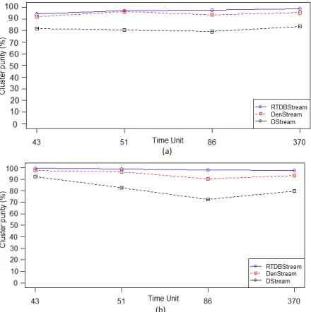
Figure 2 (a): Cluster purity of RTDBStream for EDS with H=2 and v=2000
Figure 2 (b): Cluster purity of RTDBStream for EDS with H=10 and v=2000
Figure 2 shows the purity results of RTDBStream compared to DenStream and D-Stream on EDS data
stream. In Figure 2(a), the horizon is set to 2 and stream speed v is set to 2000 points per time unit. In Figure 2(b), the horizon is set to 10 and stream speed
v is set to 2000 points per time unit. We can note that the RTDBStream shows a very good clustering quality and its clustering purity is always higher than 96%. The results show that the cluster purity of RTDBStream is higher than DenStream and D-Stream over all horizons, and in fact, purity results are insensitive to the horizon length.
[image:8.612.314.534.334.555.2]We also compared RTDBStream with DenStream and D-Stream on the Network Intrusion Detection data set. The evaluation is determined based on the selected time intervals when some attacks happen. In order to have a fair comparison, we have used the same time intervals and performed clustering as in [11]. The comparison results are shown in Figure 3. The results show that the cluster purity of RTDBStream is always above 94% and it is higher than DenStream and D-Stream over all horizons.
Figure 3. Cluster purity of RTDBStream for Network Intrusion Detection data set with (a) H=2 and v=1000
and (b) H=5 and v=1000.
4.3 Scalability Results
Execution Time: The efficiency of the
[image:8.612.91.294.350.515.2] [image:8.612.97.288.542.673.2]3981 execution time in seconds for Network Intrusion data set.
Figure 4. Execution time vs. length of stream
We can note that the execution time of RTDBStream and other methods grow linearly as the stream proceeds. We can also see that the RTDBStream has lower execution time compared to DenStream and D-Stream. The online phase of DenStream has merging task which is time-consuming. When a new data point p arrives, it takes much time to find the suitable micro cluster. So, DenStream has higher execution time. However, RTDBStream searches only in the potential µC list and if it cannot find the suitable µC, the data point is mapped to the grid in the outlier buffer. The time complexity of RTDBStream is minimized by using the grid-based clustering. It allows us to minimize the merging time complexity from o(µC) to o(1).
Memory Usage: We use both EDS data stream and
Network Intrusion Detection to evaluate the memory usage of RTDBStream. The memory usage of RTDBStream is o(µC+g) which is measured by the number of micro-clusters and grids.
4.4 Sensitivity Analysis
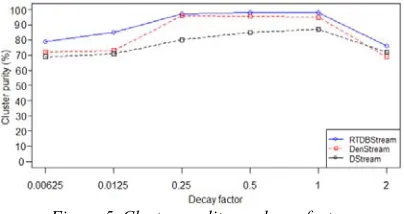
An important parameter of RTDBStream is the decay factor . The decay parameter controls the importance of historical/old data. We test the clustering quality on different values of varying from 0.0065 to 2. Figure 5 shows the results.
Figure 5. Cluster quality vs. decay factor
When is set to relatively too small or too high, the clustering quality becomes very poor. For example, when = 0.0065, the clustering purity is about 80%, and when = 2, the points decay rapidly after their
arrival, and only a few number of recent data points contribute to the final results. So the result is also very poor. However, the quality of RTDBStream is still greater than the existing methods. It can be noted that if the value of varies from 0.25 to 1, the quality of clusters is quite good, stable, and always greater than 96%.
5. DISCUSSION
Regarding the impact of our proposed algorithm, we can observe that our proposed algorithm has addressed the problems of existing algorithms. The existing algorithms for clustering data streams have high computation time and require more memory for clustering process. The experimental results of our proposed algorithm show that the RTDBStream takes less memory and computation time for clustering process. This is because, a potential micro-cluster is used to maintain summary statistics of the data stream, and a grid structure is used to map the outlier data points. It should be noted that the quality obtained by RTDBStream is higher than DenStream and D-Stream. Our algorithm is applicable for clustering real-time streaming data in a dynamic environment.
6. CONCLUSION
In this paper, we have presented RTDBStream, an efficient hybrid density-based clustering algorithm for evolving data streams. The algorithm consists of an online component for processing the incoming data and an offline component in which arbitrary shape clusters are formed using micro-clusters by a modified DBSCAN. Our algorithm uses density micro-clustering and density grid-based clustering to find high-quality clusters with considerably less computation time and memory. Experiments were conducted on synthetic and real data sets, to evaluate the performance of RTDBStream in various aspects. The evaluation results show that the proposed method has high quality and low computation time compared to existing methods. Future work will focus on extending the RTDBStream for a distributed framework and to handle high-dimensional data in an effective manner.
REFERENCES:
[1] Hahsler M, and Matthew B. Clustering Data Streams Based on Shared Density Between Micro Clusters. IEEE Transactions on Knowledge and Data Engineering, 2016. [2] Amineh Amini, Teh Ying Wah, and Hadi
[image:9.612.95.297.571.678.2]3982 Clustering Algorithms: A Survey. Journal of Computer Science and Technology, Jan. 2014, pp. 116-141.
[3] R Mathur, Integrating Big Data in Cloud Environment: A Review. (IJIET- 2016) International Journal of Innovation in Engineering and Technology. 2016, pp. 513– 517.
[4] Forsyth C, For Big Data Analytics there’s no Such Thing as Too Big. 2012 White Paper. [5] Han, J. & Kamber, M. Data Mining Concepts
and Techniques. 2006, 2nd Ed. Burlington: Morgan Kauffman.
[6] Ester, M., Kriegel, H., Sander, J. & Xu, X. A Density-Based Algorithm for Discovering Clusters in Large Spatial Databases with Noise. In: Proc. of 2nd International Conference on Knowledge Discovery, 1996, pp. 226–231.
[7] Zhou S, Zhao Y, Guan J, & Huang J. A Neighborhood-Based Clustering Algorithm. In Pacific-Asia Conference on Knowledge Discovery and Data Mining 2005, pp 361-371. [8] Ankerst, M., Breunig, M.M., Kriegel, H.-P. & Sander, J. OPTICS: Ordering Points to Identify the Clustering Structure. ACM SIGMOD Record, 1999, 28 (2). p.pp. 49–60.
[9] Hinneburg, A. & Keim, D.A. An Efficient Approach to Clustering in Large Multimedia Databases with Noise. In: KDD’98, 1998, New York, NY, pp. 58–65.
[10] Zhang T, Ramakrishnan R, Livny M. BIRCH: An efficient data clustering method for very large databases. In Proc. ACM SIGMOD International Conference on Management of Data, June 1996, pp.103-114.
[11] Cao F, Ester M, Qian W, Zhou A. Density-Based Clustering Over an Evolving Data Stream with Noise. In Proc. the SIAM Conference on Data Mining, April 2006, pp.328-339.
[12] Tasoulis D K, Ross G, Adams N M. Visualising the Cluster Structure of Data Streams. In Proc. the 7th International Conference on Intelligent Data Analysis, Sept. 2007, pp.81- 92.
[13] Menasalvas E, Ruiz C, Spiliopoulou M. C-DenStream: Using Domain Knowledge on a Data Stream. In Proc. the 12th International Conference on Discovery Science, Oct. 2009, pp.287-301.
[14] Jing K, Liu L, Guo Y et al. A Three-Step Clustering Algorithm over an Evolving Data Stream. In Proc. the IEEE Int. Conf. Intelligent Computing and Intelligent Systems, Nov. 2009, pp.160-164.
[15] Ren J, Ma R. Density-Based Data Streams Clustering over Sliding Windows. In Proc. the 6th Int. Conf. Fuzzy systems and Knowledge Discovery, Aug. 2009, pp.248-252.
[16] Lin J, Lin H. A Density-Based Clustering over Evolving Heterogeneous Data Stream. In Proc. The 2nd Int. Colloquium on Computing, Communication, Control, and Management, Aug. 2009, pp.275-277.
[17] Dunham M, Isaksson C, Hahsler M. SOStream: Self Organizing Density-Based Clustering over Data Stream. In Lecture Notes in Computer Science 7376, Perner P (ed.), Springer Berlin Heidelberg, 2012, pp.264-278. [18] Zimek A, Ntoutsi I, Palpanas T et al.
Density-Based Projected Clustering over High Dimensional Data Streams. In Proc. The 12th SIAM Int. Conf. Data Mining, April 2012, pp.987-998.
[19] Spaus P, Hassani M, Gaber M M, Seidl T. Density-Based Projected Clustering of Data Streams. In Proc. the 6th Int. Conf. Scalable Uncertainty Management, Sept. 2012, pp.311-324.
[20] Pizzuti C, Forestiero A, Spezzano G. A Single Pass Algorithm for Clustering Evolving Data Streams based on Swarm Intelligence. Data Mining and Knowledge Discovery, 2013, 26(1): 1-26.
[21] Li J, Gao J, Zhang Z, Tan P N. An incremental Data Stream Clustering Algorithm Based on Dense Units Detection. In Proc. the 9th Pacific-Asia Conference on Advances in Knowledge Discovery and Data Mining, May 2005, pp.420-425.
[22] Chen Y, Tu L. Density-Based Clustering for Real-Time Stream Data. In Proc. the 13th ACM SIGKDD Int. Conf. Knowledge Discovery and Data Mining, Aug. 2007, pp.133-142.
[23] Tan C, Jia C, Yong A. A Grid and Density-Based Clustering Algorithm for Processing Data Stream. In Proc. the 2nd Int. Conf. Genetic and Evolutionary Computing, Sept. 2008, pp.517-521.
[24] Chen Y, Tu L, Stream Data Clustering Based on Grid Density and Attraction. ACM Transactions on Knowledge discovery Data, 2009, 3(3): Article No. 12.
[25] Ng W K, Wan L, Dang X H et al. Density-Based Clustering of Data Streams at Multiple Resolutions. ACM Trans. Knowledge Discovery from Data, 2009, 3(3).
3983 Tree. Journal of Convergence IT, 2011, 6(1): 83-93.
[27] Yang Y, Liu Z, Zhang J et al. Dynamic Density-Based Clustering Algorithm over Uncertain Data Streams. In Proc. the 9th Int. Conf. Fuzzy Systems and Knowledge Discovery, May 2012, pp.2664-2670.
[28] Teh Ying W, Amini A, DENGRIS-Stream: A Density-Grid Based Clustering Algorithm for Evolving Data Streams over Sliding Window. In Proc. International Conference on Data Mining and Computer Engineering, Dec. 2012, pp.206-210.
[29] Kaur S, Bhatnagar V, Chakravarthy S. Clustering Data Streams using Grid-Based Synopsis. Knowledge and Information Systems, June 2013.
[30] Bifet, Holmes, R. Kirkby, and Pfahringer. MOA: Massive Online Analysis. J. Mach. Learn. Res., 11:1601-1604, 2010
[31] C. C. Aggarwal, Han J, Wang J, and P. S. Yu. A framework for clustering evolving data streams. In Proc. VLDB, pages 81-92, 2003. [32] Amineh Amini, Hadi Saboohi, Teh YingWah,