This is a repository copy of Candidate localness and voter choice in the 2015 General Election in England.
White Rose Research Online URL for this paper: http://eprints.whiterose.ac.uk/112489/
Version: Accepted Version
Article:
Evans, J orcid.org/0000-0001-8335-9630, Arzheimer, K, Campbell, R et al. (1 more author) (2017) Candidate localness and voter choice in the 2015 General Election in England. Political Geography, 59. pp. 61-71. ISSN 0962-6298
https://doi.org/10.1016/j.polgeo.2017.02.009
© 2017 Elsevier Ltd. This manuscript version is made available under the CC-BY-NC-ND 4.0 license http://creativecommons.org/licenses/by-nc-nd/4.0/
[email protected] https://eprints.whiterose.ac.uk/
Reuse
Items deposited in White Rose Research Online are protected by copyright, with all rights reserved unless indicated otherwise. They may be downloaded and/or printed for private study, or other acts as permitted by national copyright laws. The publisher or other rights holders may allow further reproduction and re-use of the full text version. This is indicated by the licence information on the White Rose Research Online record for the item.
Takedown
If you consider content in White Rose Research Online to be in breach of UK law, please notify us by
1
Candidate localness and voter choice in the 2015 General Election in England†
Jocelyn Evansa,*, Kai Arzheimerb, Rosie Campbellc, Philip Cowleyd
a,* School of Politics and International Studies, University of Leeds, Leeds LS2 9JT,
UK [email protected] [Corresponding author] tel: +44 (0)113 343 3681
b University of Mainz, 55099 Mainz, Germany [email protected]
c Dept. of Politics, Birkbeck, University of London WC1E 7HX, UK
d School of Politics and International Relations, Queen Mary, University of London,
E1 4NS, UK [email protected]
†Replication data for this article are available at:
http://dx.doi.org/10.17632/68gjtfg94z.1
Acknowledgements
The authors gratefully acknowledge the support of a Thyssen Foundation grant
2
Candidate localness in 2015 UK General Election
Abstract
Previous research has demonstrated a significant relationship between the
geographical distance from a voter to a candidate and the likelihood of the voter
choosing that candidate. However, models of this relationship may be mis- or
under-specified, by not taking into account voters’ perceptions of distance or not controlling
for other possible factors related to a candidate’s‘localness’ which may influence
vote choice. Using a two-wave panel survey carried out during the 2015 UK General
Election, this article tests a more fully specified alternative-specific multinomial probit
model of candidate-voter distance. We show that, although the effect size is smaller
than in previous tests, candidate-voter distance mattered in the 2015 General
Election, an effect that is robust to controls not only for party support and
incumbency, as previous research had demonstrated, but also to measures of voter
information, candidate presence and marginality. We also find that contiguity
mattered: candidates living in non-neighbouring constituencies have a lower
likelihood of vote than those living in neighbouring constituencies or in the
constituency itself.
Keywords
3
INTRODUCTION
A growing literature has shown that it matters where election candidates live (Cutler
2002; Dudley and Rapoport, 1989; Gallagher, 1980; Garand, 1988; Key 1949;
Meredith 2013a; 2013b; Rice and Macht, 1987; Studlar and McAllister 1996).
Building on ecological analyses from the 1970s onwards, which looked at candidate
and party vote-shares by broad territorial location, newer approaches have used
micro-level data to assess voters’ decision-making as a function of the precise
geographic distance between voter and candidate (Arzheimer and Evans 2012, 2014;
Gorecki and Marsh, 2012, 2014).
Yet such distance-based models have potentially been wrongly or under-specified.
First, they mostly rely upon objective measures of distance – usually looking at
straight-line or driving distance, either linear or log-transformed –rather than voters’
perceptions of distance. If, for example, voters consider distance in terms of
territorial location rather than geographical distance, then measures of contiguity –
neighbouring and non-neighbouring areas – will provide a better specification than
measures of straight-line distance.
Second, they have not generally considered other factors relevant to localism in vote
choice, such as candidates’ place of origin, length of residence in the constituency,
or the extent to which such information is available to voters before they make their
choice in an election. Third, the distance that candidates live from a constituency,
and their voters, may in fact be a result of strategic appointment and location of
candidates by parties themselves, reflecting the priority of a constituency, particularly
a marginal one, as ‘winnable’ due to factors independent of geography. The
4
therefore be a measure of the closeness of the race for that seat rather than of
localness itself. In other words, the proof of importance of a candidate’s location per
se remains under-specified and potentially spuriously related to vote likelihood
through the availability of information or other aspects of electoral localism.
In the UK, the focus of this article, analysis of the 2010 General Election in England
(Arzheimer and Evans, 2012) found a significant relationship between the
geographical distance between a voter and candidate and the likelihood of vote for
that candidate, with higher likelihood of vote at smaller distances. This was
replicated in an analysis of the 2013 English County Council Elections (Arzheimer
and Evans, 2014) which, in one of the rare studies to test contiguity, also found that
a vote for a candidate living in a neighbouring Electoral Division was significantly
less likely than for one living in the Electoral Division they were contesting, but that
there was no further reduction in likelihood for candidates in non-neighbouring
Electoral Divisions. Neither test on elections in England employed other possible
localness indicators, and to our knowledge, no information variables relating to voter
perceptions of localness have been tested in the UK or elsewhere.
This article therefore seeks to extend previous analyses of distance and localism
through models which include a fuller specification of perceptions of localness, and
considers how voter information and party supply may moderate these distance
effects. We apply these to the 2015 UK General Election, looking specifically at
English constituencies, to ensure that voters have an identical set of choices across
the main parties. We start by reviewing previous approaches to distance and
localism, to consider two approaches to testing hypotheses regarding localism and
vote. We also consider alternative operationalisations of distance, and the necessary
5
whether distance retains an independent effect under these conditions, and provide
a series of simulations to examine the impact of distance and voter information on
vote.
We show that, although the effect size is smaller than in previous tests,
candidate-voter distance mattered in the 2015 General Election. This effect is robust to controls
not only for party support and incumbency, as in previous research, but also to voter
information, candidate presence and marginality. We also find that contiguity does
matter: candidates living in non-neighbouring constituencies are less electorally
attractive than those living in neighbouring constituencies or in the constituency itself.
CANDIDATE LOCALNESS AND VOTER KNOWLEDGE
Research on the effect of candidate localness – that is, evidence of a candidate’s
presence and roots, or the lack thereof, within an electoral territory – falls broadly
into two approaches: the perceptual and the behavioural. The ‘perceptual’ approach
uses opinion poll and survey data to gauge the relative importance voters attach to a
candidate or legislator being local (Johnson and Rosenblatt, 2007, Childs and
Cowley, 2011, Wagner et al, 2015) but eschews any direct tests of distance
measures or attitudes on vote. In the controlled environment of a survey, broader
definitions of localness can be explored which go beyond geographical location, and
may make reference to a candidate’s birthplace or roots (Lee and Glasure, 1995) or
the length of time a candidate has lived in an electoral region (Studlar and McAllister,
1996). The ‘perceptual’ proof relies upon voters stating or demonstrating the
6
The ‘behavioural’ approach, which includes the majority of political geographical
work to date, infers the importance of localness from election results, using
ecological models of vote share, and individual voter behaviour, testing measures of
localness (which are almost always the geolocation of the candidate), and proximity
to the electoral region, or to voters within them. Key’s work on voting in the Southern
state of the US noted the relationship between a candidate’s vote in their home
county and adjacent counties (Key, 1949: 37-8). The latent ‘friends and neighbours’
mechanism (eg. Parker, 1982; Bowler et al, 1993), whereby local candidates are
more integrated into networks in the local community, known personally or by only a
couple of degrees of separation, and therefore advantaged by personal support
unavailable to a more distant candidate, has been developed in models looking at
local patterns of support.Gorecki and Marsh (2014) distinguish between
‘neighbourhood’ effects, where individual traits are complemented and offset by the
predominant political persuasion of the area in question (for the UK, see, for example,
Crewe and Payne, 1976) and these ‘friends and neighbours’ effects.
Ecological models have looked at candidate performance by location relative to their
home location across different levels of election in the US (Tatalovich, 1975;
Lewis-Beck and Rice, 1983; Rice and Macht, 1987; Kjar and Laband, 2002; Gimpel et al,
2008), and in New Zealand and Ireland (Johnston, 1973; Johnson, 1989). More
recently, individual-level models in Ireland and the UK have looked at voter choice to
identify the effect of voter-candidate distance on vote likelihood for these candidates
(Gorecki and Marsh, 2012, 2014; Arzheimer and Evans, 2012, 2014). The
behavioural approach has not generally tried to model the causal mechanism
underlying the relationship between location and vote likelihood, instead assuming
7
empirical support from the ‘perceptual’ approach, using survey data, or artificial
election scenarios through survey experiments to reveal voters’ preferences
(Campbell and Cowley, 2014; Roy and Alcantara, 2015). More broadly, assumptions
about effectiveness of constituency service, representation, and candidates having
an affinity for their own locale are all seen as motivating voter choice (Arzheimer and
Evans, 2012: 302).
Both these approaches rely, directly or indirectly, on an assumption of knowledge on
the part of the voter. If a voter is unaware of a candidate’s residential location, this
cannot be causally related to their vote choice. The level of knowledge required to
influence the vote is less clear, however. Gorecki and Marsh control for whether a
voter has had contact with a candidate, and find this is a significant predictor of vote
(2012: 572). But, as we consider below, contact with a candidate and the increased
voter information deriving from this, may be due to higher levels of campaigning in
targeted seats (Fieldhouse et al, 1998; Denver et al, 2002; Pattie and Johnston,
2003) or more active presence in marginal constituencies by incumbents during their
term of office (Johnston et al, 2002).
Moreover, contact with a candidate in itself is neither a necessary nor a sufficient
condition for assuming knowledge of their background. Knowledge of a candidate’s
localness, and more broadly of the candidate at all, could derive from multiple
sources. Whilst detailed knowledge of candidates’ locations is an unrealistic level of
awareness to expect of voters, a more general knowledge of localness could come,
like other political information, from word of mouth (see, e.g., Pattie and Johnston,
2000), campaign literature, local media, or other sources. We would expect most
voters to have, at best, limited knowledge of a candidate’s exact residential location.
8
such information is at the moment of vote, since the candidate’s address or at least
constituency of residence is listed on the ballot paper, and it would be unrealistic to
assume that the majority of voters pay much heed to this information in the brief time
they spend in the voting booth.) Furthermore, location of residence, and measures
based upon this, are only one possible facet of localness. If voters are motivated by
localism to some extent in their vote choice, candidates’ birthplaces, family roots,
place of business or other traits may well be identified as evidence of localness
(Childs and Cowley, 2011), even if current residential location is not deemed to be
local.
Previous work looking at candidate-voter distance in the UK (Arzheimer and Evans,
2012, 2014), included only partial controls, namely incumbency and social
deprivation. Incumbency mattered, but did not wash out the distance effect. In other
words, it was not just that incumbents tended to live closer to the constituency than
challengers (2012: 307). Similarly, checking for possible spuriousness through
socio-economic distance between voter and candidates being related to geographical
distance found no evidence that greater relative disparities in social position,
measured using a social deprivation index, reduced the likelihood of vote. But the
apparent effect of distance might be spurious for multiple other reasons. First, to
what extent are voters supportive of local candidates not because they actively
favour an individual located in their community, or that the candidates are locally
active and thereby generate a personal vote, but rather because a candidate located
in their community is more likely to be known to them than a candidate resident
some distance away –what Wagner et al (2015) refer to as a ‘profile’ effect? A
control for incumbency will potentially pick up some of this variance, but not that of
9
to what extent can one offset the other? Can distant candidates who nevertheless
establish a high profile in the constituency, or indeed establish their localness
through birthplace or other roots, offset their distance penalty?
A second element of under-specification in much of the work on candidate distance
comes from the absence of variables more commonly tested in the perceptual
approach to localism. A voter may not know where a candidate lives, whilst still being
fully aware of many other aspects of the candidate’s profile, such as where they
grew up or worked. The possibilities of unpacking the different aspects of localness
in any behavioural test are limited. The multifaceted nature of localness can be
tested on distance, but for birthplace, only partial data are available, and more
idiosyncratic links, such as place of work, are even less available and difficult to
quantify. We are thus restricted to looking at perceived localness, however that is
constructed, as an accompanying control for distance.
Finally, we need to test whether the distances observed are a function of party
supply and simply reflect parties targeting winnable seats (Krasno and Green, 1988)
and selecting more local candidates in these to ensure high visibility and local
contact.Whilst candidate selection, which may factor in residential location as a
selection criterion, would not necessarily bias the distance finding, candidate location
affected by choice of constituencies in which to challenge could well do. Should a
variable testing for this wash out the distance effect entirely, this would not be proof
that distance does not matter, but rather that it is a construct of party strategy.
However, the argument that voters regard more local candidates as preferable would
no longer be sustainable on this model alone. A simpler explanation would be that
candidates live closer in constituencies where their party does well (we do not need
10
controlling for marginality, this suggests that there is a voter-led dynamic beyond
simple party strategy.
Our expectations, then, can be set out relatively simply. Controlling for party
preference and incumbency, first, we expect that voters will be more likely to vote for
a candidate who is closer to them geographically than one who is more distant, other
things being equal. When location is construed by territorial contiguity rather than
distance, we expect that voters will be most likely to vote for a candidate living in the
same constituency, and that additionally they will be more likely to vote for a
candidate living in a neighbouring constituency than a non-neighbouring
constituency. Second, we expect that voters will be more likely to vote for a
candidate whom they perceive as having a higher level of localness. Third, voters
will be more likely to vote for a candidate about whom they have information. Fourth,
drawing on Gorecki and Marsh (2012), voters will be more likely to vote for a
candidate who has contacted them. Finally, we wish to see whether party strength,
and thus chances of winning a constituency, account for any or all of the distance
effect, indicating strategic positioning of candidates in areas of previous strength.
DATA AND METHOD
Information on vote, voter knowledge and party preference was collected using a
two-wave internet panel delivered by the YouGov polling organisation, resulting in a
full sample of 5972 voters in 532 of the 533 English constituencies (excluding
Buckingham, the constituency of the Speaker of the House of Commons, whose
candidacy traditionally goes unchallenged by the other main parties). The first wave
11
delivered in the week following the election on 6 May 2015. The first wave asked a
set of 11-point thermometer questions on the four main parties (Conservatives,
Labour, Liberal Democrats and UKIP), to allow us to control for overall party
preference before the beginning of the short campaign, as well as four questions
asking respondents to identify how local the candidate from each of these parties
was, on a four-point ordinal scale, or whether they did not know the level of localness.
The second wave provided the reported vote of the respondents, which is used as
the outcome variable.
To calculate voter-candidate distance, voter location is obtained from full postcode
information included in the YouGov survey. Candidate data were compiled from the
Statements of Persons Nominated (SoPNs) collected from the 532 constituencies,
which include either full postcode information or the residential constituency of the
candidate. Using the Ordnance Survey BoundaryLine™ vector shapefile and the
OS/Royal Mail Code-Point® point dataset in the QGIS software package, the
straight-line distance between voters and candidates who provided full postcode
information was calculated. We tested a fractional polynomial transformation
(Royston and Sauerbrei, 2008) of the distance effect in the model, to see if a
log-transformed or other power-log-transformed measure fitted the data better, but none
improved on the linear effect.
Contiguity measures were generated using the spdep and spatial packages in R to
identify neighbouring and non-neighbouring constituencies for each English
constituency. Different analytical sample sizes result from some candidates
providing only their residential constituency on the SoPN (and therefore on the ballot
paper), rather than their full residential address. Moreover, given the data were
12
candidates who had formally been identified by the time the respondent completed
the YouGov survey, to avoid including respondents who gave information on
non-existent candidates.We acknowledge that other information may have been received
by voters about their candidates subsequent to completing the survey, which may
then influence their eventual vote choice – a point to which we return in the
discussion – but we have no way of correcting for this potential bias. We took
candidate identification recorded in the Representative Audit of Britain 2015
Parliamentary Candidate database for this purpose. The map in Figure 1 shows the
constituencies with sufficient address information across candidates to be included in
the distance model. The contiguity model had sufficient information by constituency
to exclude only North Tyneside from the analysis, in addition to Buckingham. For the
distance models, 2409 respondents across 403 constituencies are included in the
analytical sample. Figure 1 shows the location of these constituencies. This
increases to 3902 respondents across the 531 constituencies for the contiguity
models.
[Figure 1 about here]
The effect of perceived localness is tapped using the four-point ordinal scales,
asking how local a candidate is, which we retain as separate categories to include
full information; we also include the ‘don't know’ category as a valid response, to
understand whether a lack of awareness of localness is ‘worse’ (electorally) for a
candidate than being perceived as an outsider. Including this variable together with
distance allows us to see the extent to which the perception of localness is related
13
An initial exploratory test for the objective distance and perceived localness
measures is the extent to which they are related. On average, do candidates who
are classified as ‘very local’ live closer than those classified as ‘not local at all’?
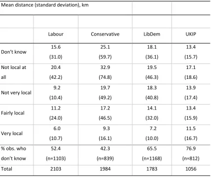
Table 1 presents the mean distance of candidates by perceived level of localness for
the four parties, and shows a clear pattern of monotonicity among the informed
responses, with the partial exception of Labour. Overall, candidates identified as
more local do indeed live closer to the voters, with those seen as ‘very local’ by
voters displaying extremely high levels of localness on average.
[Table 1 about here]
Nonetheless, the standard deviations illustrate that there is wide variation by
candidates around this mean. Moreover, there are a considerable number of voters
who say they do not know how local the candidates are: about 40% of voters were
unaware of Conservative candidates’ localness, rising to 50% for Labour, two-thirds
for Liberal Democrats and three-quarters for UKIP. This ‘Don’tKnow’ category
exhibits a lower mean than ‘not local at all’ across all four parties, and intermediate
levels of standard deviation. We might have expected the highest deviation scores
for this category, which could potentially include very proximate candidates of whom
voters are simply not aware. Finally, we should recall localness is not simply a
function of distance to residential address – high distance may not outweigh
birthplace in localness, for example.
We test information effects partly by using this same question about localness, and
retaining the ‘don’t know’ category as a valid response. But this only tests for the
effect of not knowing about the localness of a candidate – it does not test for broader
14
respondent is aware of ‘the [party] candidate’ is potentially uninformative, or worse,
and asking respondents to name each candidate is unrealistic in requiring a higher
degree of active knowledge, we instead use an aggregate index to measure the
degree of activity of a candidate in a constituency, and voters’ awareness of the
candidate. We test two versions of this. The first, from the same YouGov survey, is
an average index measuring knowledge of each candidate based upon all
respondents from a constituency. Other things being equal, we assume that in a
constituency where more respondents proffer a response as to the level of localness
of a give candidate, the greater the average knowledge of the candidate more
generally, and therefore the higher the likelihood of individual vote choice,
irrespective of knowledge of localness.
A second version of this test uses data from Wave 5 of the British Election Study
(BES), carried out between 31 March and 6 May 2015 and sampling 22,204 English
respondents, which asked people if they had been contacted by each of the main
parties during the campaign. A number of different modes of contact are specified by
the BES, but we restrict ourselves to using contact by leaflet – by far the most
common form of campaign information dissemination (Cowley and Kavanagh, 2015:
273), and the one most likely to contain positive information about the party
candidate, as well as information about the localness of the candidate. We calculate
the proportion of respondents surveyed by the BES in each constituency who state
that they received a campaign leaflet, and from which party. This proportion is then
matched to individual respondents in our YouGov dataset by party and by
constituency. Given the large sample size of the BES across constituencies, we see
this as an adequate measure of the relative extent of leafletting in the constituency.
15
disseminating candidate information in a constituency, will increase the probability of
vote for that party’s candidate.
We checked for a relationship between level of contact and distance, to understand if
the level of leafletting was strongly determined by the proximity of the candidate to
their constituency. Correlation coefficients were weak but significant for
Conservatives (-0.17), Labour (-0.09) and Liberal Democrats (-0.13), and absent for
UKIP (0.04). The inclusion of both variables in the models poses no issue.
Finally, to test the effect of party supply, and the chance of winning a constituency
for each of the four parties, we use a measure of marginality that is based on the
2010 results. Parties put in greater resources to marginal constituencies than to safe
seats, to increase their candidate’s competitiveness. We measure this using the
difference between the vote share for the party of the candidate in question and the
winning party, or the party and the second-placed party in the case of winning
candidates themselves. This results in a folded scale bounded by 0 and 100. Whilst
party strategy in targeting seats is more complicated than simply identifying marginal
constituencies where the party is well placed, it is difficult to reflect this complexity. It
does, however, require the loss of some observations due to the absence of a UKIP
candidate in 2010.
We run a series of alternative-specific multinomial probit (ASMP) models, predicting
vote likelihood for each of the four main parties, using a set of explanatory variables
for which there is a different score by candidate. ASMP models choice data including
both case-specific variables (such as a respondent’s age or gender) and alternative
-specific variables, which will normally vary across both cases and alternatives (a
16
candidates). As with the better-known multinomial probit (MNP) model, one picks an
arbitrary alternative (Labour in our case) as the reference category to identify the
model. A crucial difference between the MNP and ASMP models is that the latter
treats the choices each respondent (or case) made regarding the four main parties
as observations, producing a stacked data matrix of multiple observations per case.
Because the observations are not independent – since choices for/against the main
parties are 'nested' within choosers – standard errors are corrected accordingly, as
well as for clustering by constituency.
In reality, the number of observations is considerably smaller than the number of
respondents multiplied by four, because some respondents have missing values for
a single choice (the respondent did not rate one of the parties on the thermometer
scale, for example), one of the candidates did not provide their full address on the
SoPN (so distance cannot be calculated), or because the respondent did not vote for
one of the main parties so that there is no variation between the four possible
choices that could be modelled.
Previous research has used conditional logit models, as these are the most
prominent statistical method for analysing choice data. One potential concern with
the conditional logit model, however, is the assumption of independence from
irrelevant alternatives (IIA). The IIA assumption states that the odds of preferring
party A over party B are not affected if new parties are added to the choice set or
existing parties are removed. In the context of electoral choice, IIA would be violated
if some party C was seen as a perfect substitute for either A or B by voters. While
the validity of the IIA assumption can be formally tested, Monte Carlo experiments
have shown that the three most popular tests - the McFadden, Train, and Tye Test,
17
and have poor properties even in large samples (Cheng and Long 2007). Cheng and
Long therefore argue that that one should follow McFadden's (1973: 113) early
advice to treat the IIA not merely as a technical, but also as a substantive question:
that is, to restrict multinomial and conditional logit analysis to situations where
choices are perceived as "distinct ... by each decision maker".
Using ASMP takes an additional precaution again the IIA problem, as it assumes
that the error terms in the model have a multivariate normal distribution that is both
heteroskedastic and potentially correlated. Consequently, the odds of picking one
alternative may vary dependent upon the other available choices, and the IIA
assumption does not apply. The barrier to the use of ASMP has been computational,
given its reliance upon simulation techniques to establish the maximum likelihood
estimates for the parameters of the model. Achieving convergence in estimations for
our models proved unproblematic, and interestingly, the findings were largely
mirrored by those from the equivalent conditional logit model (see Appendix A). This
conforms to Dow and Endersby’s finding (2004) that the IIA rarely poses a problem
using election data from free multi-party elections such as those in the UK.
In each model, the outcome variable is vote, coded across the four possible choices
– Labour, Conservative, Liberal Democrat and UKIP. Models 1a and b introduce
candidate location measures with standard controls. We use two different location
models: the distance model 1a, which measures the straight-line distance between
the voter’s home address and that of the candidate; and the contiguity model 1b,
with a factor variable coded 1 for candidates living in a neighbouring constituency to
the voters, and coded 2 for candidates living in a non-neighbouring constituency
(with home constituency being the reference). Standard controls for party and
18
for each of the four main parties, and a dummy variable coded 1 for incumbent
candidate by constituency.
Models 2a and 2b introduce the localness variable, to look at the extent to which
perceptions of localness of a candidate matter independently from distance. Our
findings in Table 1 lead us to expect that distance should remain significant, with
variance explained by other elements of localness picked up by the relevant level of
localness. In the final two models, 3a and 3b, we include the party contact and profile
indices, and the measure of marginality, to look at the extent to which distance and
localness may simply be reflecting higher levels of information. We look in particular
to see if distance and contiguity retain an independent effect on vote likelihood.
Overall, we expect candidates to have the highest likelihood of vote if they have an
active party, a high profile in the constituency, or a high marginality – as well as if
they have a low distance to voters or live in their home constituency.
ANALYSIS
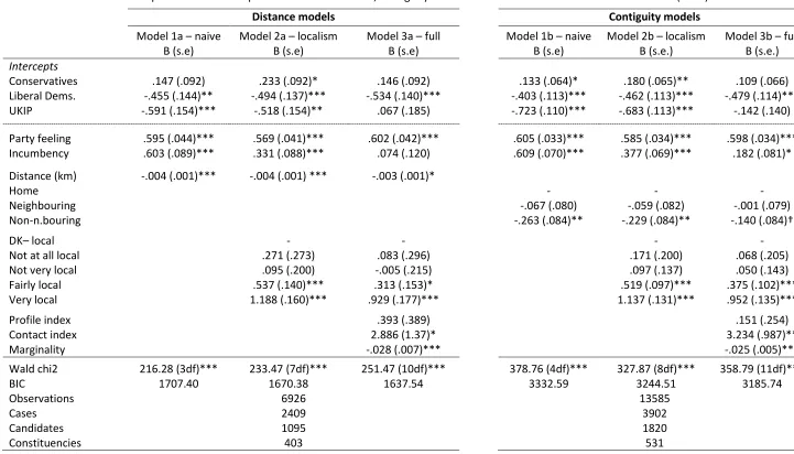
Table 2 presents the nested models for the distance and contiguity tests.
[Table 2 about here]
Models 1a and 1b broadly confirm what we expect to see, with one notable
exception. Model 1a indicates that distance matters, with candidates at higher
distances from voters less likely to receive their vote, even controlling for
incumbency and party feeling, which as we would expect are strong predictors of
vote choice. In Model 1b, candidates living in constituencies which do not neighbour
19
candidates living in their constituency. However, vote likelihood for a candidate living
in a neighbouring constituency is not significantly lower than vote for a home
candidate. Voters are no more likely to favour someone in their own constituency
than one next door. (A change in contrast to the non-neighbouring category
establishes a higher likelihood of vote for candidates in neighbouring over
non-neighbouring constituencies, significant at the 90% level.) This contrasts with the
contiguity findings for local elections in the UK, where the key difference was
between candidates in their home Electoral Division, or any other Electoral Division,
adjacent or not (Arzheimer and Evans, 2014). For national elections, contiguity
seems less restrictive, apparently.
Models 2a and 2b introduce the localness variable to the distance model. The
distance parameter remains stable and highly significant. Despite the clear
relationship between perceived localness and distance (see Table 1), there are other
elements of localness which explain variance in vote likelihood. For localness, in
contrast to the ‘don’t know’ baseline, candidates ranked as fairly local and very local
have much greater vote likelihood, other things being equal. If distance is picking up
the geographical element of this effect, other aspects such as length of residence in
the constituency, or candidates’ origins, that voters will use to construe ‘localness’
also clearly matter. Conversely, perceiving a candidate as not being local, or hardly
local, is no more or less deleterious to vote chances than not knowing their localness
at all. The size of the incumbency effect halves, demonstrating an association
between incumbency and voters’ perceptions of them as local. The results in the
contiguity model (2b) are substantively identical.
Models 3a and 3b introduce the candidate profile, candidate contact and marginality
20
itself, the effect is significant, but strong covariation between profile, contact and
marginality sees the former variable wash out in the fuller specification. While this
tells us something of interest – that voters are on average more aware of candidates
for parties standing in marginal seats and actively campaigning – it reduces the
explanatory power of the candidate profile index by itself. Of more value are the
contact and marginality indices, both of which are significant and in the expected
direction. Marginality is particularly significant – parties in closer races at the
previous election are more likely to win votes, other things being equal. Looking at
the contact variable, higher levels of constituency contact by the party or candidate
on average increase the probability of vote.
There is also an association between incumbency and candidate knowledge – in the
distance model sample, incumbents average a candidate profile index of 0.64,
against non-incumbents’ 0.30 – but much less so between incumbency and contact
by leaflet (.20 for incumbents, .12 for non-incumbents). Incumbents have a built-in
profile advantage through constituency service and established networks – a key
element of the ‘friends and neighbours’ vote – but challengers may campaign as
strongly, or more so, and this works to their advantage in raising the probability of
vote. The inclusion of these two variables sees incumbency lose significance.
Most importantly for this analysis, the distance effect diminishes but remains
significant at the 95% level. If parties are placing local candidates in target
constituencies, this does not entirely pre-determine distance, nor does information
about the candidate from contact eliminate this. This provides strong evidence that
the location of the candidate does matter, together with other aspects of localness,
21
Running the contiguity model with the contact, profile and marginality variables in
Model 3b, the effect of these is very similar to the distance model. However, the
contiguity effect attains significance only at the 90% level in Model 3b. This is
unlikely to be a sample-size related Type II error. Running the model with only the
non-neighbouring contrast included makes little difference to the effect size or
significance. Similarly, the reduction in significance does not appear to be due to
noise introduced by previous redistricting of incumbents, for example – interaction
effects between incumbency and contiguity confirm the null. One possible issue may
be the effect of the geographical size of constituency – for small, urban
constituencies, a non-neighbouring constituency may be closer than parts of a
neighbouring constituency in a large rural area. Given the lack of within-group
variation on constituency size, it is impossible to include this in the probit model.
However, if we run separate models (not shown) for small and large constituencies,
using mean area in hectares as the cut-off, an effect almost significant at the 99%
level and in the expected direction is found for non-neighbouring constituencies in
the larger constituencies, even when controlling for profile, contact and marginality.
Lastly, unlike the distance model, incumbency remains significant and with a larger
parameter point estimate. Given the model includes the same control variables as in
Model 3a, this must be related to the additional constituencies and cases included
through contiguity, but we have been unable to identify why incumbency should
retain an effect in constituencies where more candidates withhold their addresses.
[Table 3 about here]
Previous work has provided simulations showing how vote likelihood varies by
22
we cannot compare directly with the 2010 election, since in previous work voter
locations were estimated by ward centroid due to data restrictions on precise
geolocation. Moreover, we wish to look at the effect of distance in a more robust
model where candidate information and campaign behaviour have been included.
We will therefore briefly consider 2015 estimates using an approximation of the 2010
model.
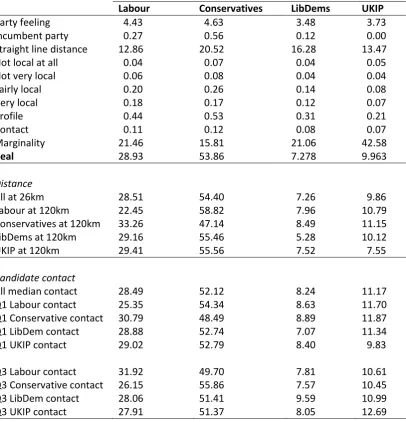
In the upper half of Table 3, we first look at vote probabilities when all candidates are
placed at 26km from a notional voter, and then in turn we move each party’s
candidate to 120km from the voter, leaving the other three parties at 26km. These
are the distances which were originally tested in the earlier 2010 analysis (Arzheimer
and Evans, 2012: 308, table 3). The top section gives the mean scores and
proportions of the other variables in the model, with the ‘Real’ row giving the actual
vote probabilities from the analytical sample. The size of change is conditional upon
the baseline probability for the party, with no evidence of differential effects by party
when these were tested using interactions between party and distance. The
Conservatives lose around 7 percentage points if their candidate is placed
substantially further away, compared to a situation where all candidates are placed
equally distant. Under equivalent scenarios, Labour lose around 6 percentage points,
and Liberal Democrats and UKIP around 2 points. Graphing probabilities and
marginal effects revealed a clearly linear effect (see Appendix B).
This Conservative effect compares with an estimate of around 16 percentage points
in the 2010 General Election (Arzheimer and Evans, 2012: 308). Given the
difference in choice set, voter location estimation, model specification and
measurement of distance – driving distance was used in the 2010 test – we also
23
UKIP as a choice response, and localness and contact as explanatory variables, and
estimating driving-distance from straight-line distance by regression on 2010 scores,
but the simulation estimates remained very similar (see Appendix C). We have no
reason to suspect that a distance effect should be greater in the context of the 2010
elections and consequently, we are left with an unstable distance effect across time.
We return to this in the discussion.
In the lower section of Table 3, we look at the effect of candidate contact on vote
share, to compare with the distance simulations. We look first at the vote
probabilities if candidate for all parties are set to the median proportion of leafletting.
We then in turn raise each party’s leafletting to the upper quartile proportion, holding
the others at the median, and then lower each party to the lower quartile proportion.
For the Conservatives, lower levels of campaigning result in around a 3.5 percentage
point drop, and a similar rise for higher campaigning. Similar changes affect the
other parties proportionate to their baseline probability. Labour drops or gains around
3 points due to low or high contact, respectively. Liberal Democrats and UKIP
variation is just over +/- 1 point. Contact through leaflets, then, makes a difference,
but not sufficient to offset concerns over localness. Other things being equal, a
relatively inactive candidate with strong local credentials will perform better than a
distant candidate with strong campaigning.
DISCUSSION
The distance effect found in 2010 thus persists in 2015, even when included in a
much more fully specified model accounting for other aspects of localness and voter
24
be regarded as a ‘game-changer’ under normal circumstances, and the instability of
the parameter estimate is noticeable across the two election years. But although a
host of other explanations of voter choice are controlled via the thermometer
instrument, and although the candidates’ individual incumbency status is accounted
for, too, the location of a candidate relative to her voters still has a bearing on the
likelihood of them voting for her, and this difference in 2015, as in 2010, could
potentially be crucial in marginal constituencies, particularly if parties maximise other
information and campaign effects.
An alternative mode of construing distance, contiguity, similarly finds support. Voters
prefer candidates to be placed in a more local environment – the constituency or a
neighbouring one – to further afield. However, once information and contextual
effects have been controlled for, this effect weakens more than is the case for the
distance variable. While contiguity might perhaps be closer to how we would expect
voters to perceive proximity of candidates, given it relies on distinct areas rather than
precise distance, the heterogeneity in constituency size and its weaker influence in
the fully specified model would still lead us to favour distance as the simplest,
consistent measure.
Other aspects of localness clearly matter too. We have been unable to unpick these
here from the voter perceptions, but our findings suggest empirical tests of such
things as candidate origins and ‘rootedness’ are worth pursuing. Distance matters as
it affects voter knowledge, and it is also an indirect manifestation of party strategy in
(un)winnable seats, but it also matters independently as a heuristic for candidate
25
Indeed, in some ways the persistence of a distance effect is the most striking finding,
given that the evidence suggests that, with the exception of the Conservative Party,
the majority of voter-candidate pairs result in a ‘Don’t Know’ for candidate localness.
As we noted at the beginning of the article, one possibility is that our survey
respondents received more information, including some indication of localness, in
the short campaign one month before the election. In this case, a higher proportion
would be aware of location, and this would account for distance mattering in the face
of locational ignorance at the time of the survey. Another necessarily speculative
explanation would be that some other mechanism still underlies distance, which we
have not picked up with our controls. These two possible explanations suggest very
different conclusions for the distance effect – the first positive, the second negative.
Both are weaknesses which we would strive to correct in subsequent testing.
Whilst the inclusion of information and contact effects provides an improved
specification of distance models, there are clearly other elements to candidate
location which remain to be examined. The next step should be to include a full
specification of all candidate traits, including gender (Dolan, 2004), occupation
(Mechtel, 2011) and ethnicity (Fisher et al, 2014), as well as attractiveness (Mattes
and Milazzo, 2014). We see no a priori reason to expect that the effect of distance
will vary by these traits, so believe that our model remains robust without them.
Similarly, traits in voters, as causal priors to political sophistication, may condition the
effect of distance, if use of location information is either the mark of a sophisticated
voter, or a variable which the sophisticated voter eschews in favour of alternative
indicators of competence and suitability. Lacking a suitable measure of political
26
In short, the robustness of the distance effect to controls for information and
candidate profile, party supply, as well as broader manifestations of localness, does
not settle the argument regarding its independence. However, it does provide
stronger evidence that the importance of localness to voters in their representatives
manifests itself through their location, as well as other aspects of their rootedness in
27
REFERENCES
Arzheimer, K. and Evans, J. (2012). Geolocation and voting: candidate-voter
distance effects on party choice in the 2010 UK general election in England.
Political Geography, 31(5), 301-310.
Arzheimer, K. and Evans, J. (2014). Candidate geolocation and voter choice in the
2013 English County Council elections. Research and Politics, July-September,
1(2).
Bowler, S., Donovan, T., and Snipp, J. (1993). Local sources of information and
voter choice in State elections: microlevel foundations of the "friends and
neighbors" effect, American Politics Research, 21(4), 473-489.
Campbell, R. and Cowley, P. (2014). What voters want: reactions to candidate
characteristics in a survey experiment. Political Studies, 62(4), 745-65.
Cheng, S. and Long, J.S. (2007). Testing for IIA in the multinomial logit model.
Sociological Methods & Research, 35(4), 583-600.
Childs, S. and Cowley, P. (2011). The politics of local presence: is there a case for
28
Cowley, P. (2013). Why not ask the audience? Understanding the public's
representational priorities. British Politics, 8(2), 138-63.
Cowley, P. and Kavanagh, D. (2015). The British General Election of 2015, London:
Palgrave.
Crewe, I. and Payne, C. (1976). Another game with nature: an ecological regression
model of the British two-party vote ratio in 1970. British Journal of Political
Science, 6(1), 43–81.
Cutler, F. (2002). The simplest shortcut of all: sociodemographic characteristics and
electoral choice. The Journal of Politics, 64(2), 466-90.
Denver, D., Hands, G., Fisher, J., & McAllister, I. (2002). The impact of constituency
campaigning in the 2001 general election. In L. Bennie, C. Rallings, J. Tonge, & P.
Webb (Eds.), British elections and parties review 12: the 2001 General Election.
London: Frank Cass, 80-94.
Dolan, K. (2004) Voting for Women: How the Public Evaluates Women Candidates,
29
Dudley, R. and Rapoport, R. (1989). Vice-Presidential candidates and the home
state advantage: playing second banana at home and on the road. American
Journal of Political Science, 33(2), 537-40.
Dow, J. and Endersby, J. (2004). Multinomial probit and multinomial logit: A
comparison of choice models for voting research. Electoral Studies, 23(1),
107-122.
Fieldhouse, E., Pattie, C., & Johnston, R. (1996). Tactical Voting and Party
Constituency Campaigning at the 1992 General Election in England. British
Journal of Political Science, 26(3), 403-418.
Fisher, S. D., Heath, A. F., Sanders, D., & Sobolewska, M. (2014). Candidate
ethnicity and vote choice in Britain. British Journal of Political Science, 45(4), 1-23.
Gallagher, M. (1980). Candidate selection in Ireland: the impact of localism and the
electoral system. British Journal of Political Science, 10(4): 489-503.
Garand, J. (1988). Localism and regionalism in Presidential elections: is there a
home state or regional advantage. The Western Political Quarterly, 41(1),
30
Gimpel, J. G., Karnes, K. A., McTague, J., & Pearson-Merkowitz, S. (2008).
Distance-decay in the political geography of friends-and-neighbors voting. Political
Geography, 27(2), 231-252.
Gorecki, M. A., and Marsh, M. (2012). Not just ‘friends and neighbours’: canvassing,
geographic proximity and voter choice. European Journal of Political
Research, 51(5), 563-582.
Górecki, M. A., and Marsh, M. (2014). A decline of ‘friends and neighbours voting’ in
Ireland? Local candidate effects in the 2011 Irish ‘earthquake election'. Political
Geography, 41, 11-20.
Johnson, C. and Rosenblatt, G. (2007). Do MPs have the ‘Right Stuff? Parliamentary
Affairs, 60(1), 164-9.
Johnson, N. (1989). An analysis of the ‘friends and neighbours’ effect in an Irish
urban constituency. Irish Geography, 22(2), 93–105.
Johnston, R. (1973). Spatial patterns and influences on voting in multi-candidate
elections: the Christchurch City Council election, 1968. Urban Studies, 10 (1),
31
Johnston, R., Cowley, P., Pattie, C. and Stuart, M. (2002). Voting in the House or
wooing the voters at home: Labour MPs and the 2001 General Election campaign.
Journal of Legislative Studies, 8(2), 9-22.
Key, V.O. (1949) Southern Politics in State and Nation. New York: Vintage.
Kjar, S. and Laband, D. (2002). On “home grown-ness” in politics: evidence from the
1998 election for Alabama’s Third Congressional District. Public Choice, 112(1-2),
143-150.
Krasno, J. and Green, D. (1988). Preempting quality challengers in House elections.
The Journal of Politics, 50(4), 920-36.
Lee, A.-R. and Glasure, Y. (1995). Party identifiers in South Korea: differences in
issue orientations. Asian Survey, 35(4), 367-376.
Lewis-Beck, M., and Rice, T. (1983). Localism in presidential elections: the home
state advantage. American Journal of Political Science, 27(3), 548-556.
Mattes, K. and Milazzo, C. (2014). Pretty faces, marginal races: predicting election
outcomes using trait assessments of British parliamentary candidates. Electoral
32
Mechtel, M. (2011). It's the occupation, stupid! Explaining candidates' success in
low-information elections.European Journal of Political Economy 33, 53-70.
Meredith, M. (2013a). Exploiting friends-and-neighbors to estimate coattail effects.
American Political Science Review, 107(4), 742-765.
Meredith, M. (2013b). Heterogeneous Friends-and-Neighbors Voting. Unpublished
manuscript.
Parker, A. (1982). The ‘friends and neighbours’ voting effect in the Galway West
constituency. Political Geography Quarterly, 1(3), 243-262.
Pattie, C. and Johnston, R. (2000). ‘People who talk together vote together’: an
exploration of contextual effects in Great Britain. Annals of the Association of
American Geographers, 90(1), 41-66.
Pattie, C. and Johnston, R. (2003) Local battles in a national landslide: constituency
campaigning at the 2001 British General Election. Political Geography, 22(4),
381-414.
Rice, T. and Macht, A. (1987). Friends and neighbors voting in statewide general
elections. American Journal of Political Science, 31(2), 448-52.
Roy, J. and Alcantara, C. (2015). The candidate effect: does the local candidate
33
Royston, P. and Sauerbrei, W. (2008). Multivariable Model-building: A Pragmatic
Approach to Regression Analysis Based on Fractional Polynomials for Modelling
Continuous Variables. Wiley.
Studlar, D. and McAllister, I. (1996). Constituency activity and representational roles
among Australian legislators. The Journal of Politics, 58(1), 69-90.
Tatalovich, R. (1975). Friends and neighbors' voting: Mississipi 1943-73. The Journal
of Politics, 37(3), 807-14.
Wagner, M., Campbell, R., Cowley, P. and Vivyan, N. (2015). Explaining voter
preferences for local legislators: evidence from a conjoint analysis survey
experiment', paper presented at Elections, Public Opinion and Parties annual
34
[image:35.595.70.499.92.453.2]TABLES AND FIGURES
Table 1 Mean candidate-voter distance by perceived candidate localness for the four parties
Mean distance (standard deviation), km
Labour Conservative LibDem UKIP
D 15.6 (31.0) 25.1 (59.7) 18.1 (36.1) 13.4 (15.7)
Not local at
all 20.4 (42.2) 32.9 (74.8) 19.5 (46.3) 17.1 (18.6)
Not very local
9.2 (10.4) 19.7 (49.2) 18.3 (40.8) 13.9 (17.4) Fairly local 11.2 (24.0) 17.2 (46.5) 14.1 (32.0) 13.4 (15.9) Very local 6.0 (10.7) 9.3 (16.1) 7.2 (10.0) 11.5 (16.7)
% obs. who 52.4
(n=1103) 42.3 (n=839) 65.5 (n=1168) 76.9 (n=812)
35
Table 2 Alternative-specific multinomial probit models of distance, contiguity and candidate information effects on vote choice (2015)
Distance models Contiguity models
Model 1a naive Model 2a localism Model 3a full Model 1b naive Model 2b localism Model 3b full
B (s.e) B (s.e) B (s.e) B (s.e) B (s.e.) B (s.e.)
Intercepts
Conservatives .147 (.092) .233 (.092)* .146 (.092) .133 (.064)* .180 (.065)** .109 (.066)
Liberal Dems. -.455 (.144)** -.494 (.137)*** -.534 (.140)*** -.403 (.113)*** -.462 (.113)*** -.479 (.114)*** UKIP -.591 (.154)*** -.518 (.154)** .067 (.185) -.723 (.110)*** -.683 (.113)*** -.142 (.140)
Party feeling .595 (.044)*** .569 (.041)*** .602 (.042)*** .605 (.033)*** .585 (.034)*** .598 (.034)*** Incumbency .603 (.089)*** .331 (.088)*** .074 (.120) .609 (.070)*** .377 (.069)*** .182 (.081)*
Distance (km) -.004 (.001)*** -.004 (.001) *** -.003 (.001)*
Home - - -
Neighbouring -.067 (.080) -.059 (.082) -.001 (.079)
Non-n.bouring -.263 (.084)** -.229 (.084)**
-DK local - - - -
Not at all local .271 (.273) .083 (.296) .171 (.200) .068 (.205)
Not very local .095 (.200) -.005 (.215) .097 (.137) .050 (.143)
Fairly local .537 (.140)*** .313 (.153)* .519 (.097)*** .375 (.102)***
Very local 1.188 (.160)*** .929 (.177)*** 1.137 (.131)*** .952 (.135)***
Profile index .393 (.389) .151 (.254)
Contact index 2.886 (1.37)* 3.234 (.987)**
Marginality -.028 (.007)*** -.025 (.005)***
Wald chi2 216.28 (3df)*** 233.47 (7df)*** 251.47 (10df)*** 378.76 (4df)*** 327.87 (8df)*** 358.79 (11df)***
BIC 1707.40 1670.38 1637.54 3332.59 3244.51 3185.74
Observations Cases Candidates Constituencies
6926 2409 1095 403
13585 3902 1820 531
36
Table 3 Simulations of vote share with variable candidate distance and campaign contact
Labour Conservatives LibDems UKIP
Party feeling 4.43 4.63 3.48 3.73
Incumbent party 0.27 0.56 0.12 0.00
Straight line distance 12.86 20.52 16.28 13.47
Not local at all 0.04 0.07 0.04 0.05
Not very local 0.06 0.08 0.04 0.04
Fairly local 0.20 0.26 0.14 0.08
Very local 0.18 0.17 0.12 0.07
Profile 0.44 0.53 0.31 0.21
Contact 0.11 0.12 0.08 0.07
Marginality 21.46 15.81 21.06 42.58
Real 28.93 53.86 7.278 9.963
Distance
All at 26km 28.51 54.40 7.26 9.86
Labour at 120km 22.45 58.82 7.96 10.79
Conservatives at 120km 33.26 47.14 8.49 11.15
LibDems at 120km 29.16 55.46 5.28 10.12
UKIP at 120km 29.41 55.56 7.52 7.55
Candidate contact
All median contact 28.49 52.12 8.24 11.17
Q1 Labour contact 25.35 54.34 8.63 11.70
Q1 Conservative contact 30.79 48.49 8.89 11.87
Q1 LibDem contact 28.88 52.74 7.07 11.34
Q1 UKIP contact 29.02 52.79 8.40 9.83
Q3 Labour contact 31.92 49.70 7.81 10.61
Q3 Conservative contact 26.15 55.86 7.57 10.45
Q3 LibDem contact 28.06 51.41 9.59 10.99
38
Appendix A Conditional logit models of distance, contiguity and candidate information effects on vote choice (2015)
Distance models Contiguity models
Model 1a naive Model 2a localism Model 3a full Model 1b naive Model 2b localism Model 3b full
B (s.e) B (s.e) B (s.e) B (s.e) B (s.e.) B (s.e.)
Intercepts
Conservatives .165 (.108) .267 (.107)* .161 (.106) .136 (.076) .204 (.076)** .103 (.077)
Liberal Dems. -.405 (.126)** -.474 (.120)*** -.496 (.131)*** -.368 (.102)*** -.432 (.098)*** -.482 (.103)*** UKIP -.567 (.155)*** -.439 (.147)** .259 (.190) -.712 (.102)*** -.619 (.100)*** .077 (.146)
Party feeling .748 (.033)*** .714 (.032)*** .729 (.033)*** .759 (.023)*** .725 (.023)*** .737 (.023)*** Incumbency .771 (.107)*** .436 (.103)*** .188 (.137) .776 (.079)*** .496 (.078)*** .269 (.095)**
Distance (km) -.005 (.001)*** -.004 (.001)*** -.003 (.001)**
Home - - -
Neighbouring -.051 (.092) -.041 (.092) .038 (.089)
Non-n.bouring -.263 (.099)** -.227 (.098)* -.127 (.099)
DK local - - - -
Not at all local .191 (.292) -.001 (.314) .151 (.239) .032 (.247)
Not very local .223 (.248) .141 (.253) .167 (.168) .111 (.172)
Fairly local .691 (.163)*** .437 (.175)* .615 (.113)*** .448 (.119)***
Very local 1.439 (.185)*** 1.139 (.201)*** 1.325 (.140)*** 1.108 (.148)***
Profile index .233 (.453) .173 (.301)
Contact index 3.234 (1.530)* 3.524 (1.145)**
Marginality -.033 (.008) -.032 (.006)***
Wald chi2 624.34 (6df)*** 634.21 (10df)*** 665.32 (13df)*** 1319.89 (7df)*** 1287.45 (11df)*** 1325.99 (14df)***
BIC 1637.106 1598.252 1572.908 3251.522 3171.449 3116.277
Observations Cases Candidates Constituencies
6926 2409 1095 403
13585 3902 1820 531
39
Appendix B Fitted probability and marginal effects graphs of distance on vote choice by party
.2 7 .2 8 .2 9 .3
0 10 20 30 40
probability of choosing Labour
-.
0
0
1
2 -.0
0 1 -. 0 0 0 8-. 0 0 0 6-. 0 0 0 4-. 0 0 0 2
0 10 20 30 40
Distance (km)
marginal effect of Labour distance and 95% confidence interval
.5 2 .5 3 .5 4 .5 5 .5 6
0 10 20 30 40
probability of choosing Conservative 0 .0 0 0 2 .0 0 0 4 .0 0 0 6 .0 0 0 8 .0 0 1
0 10 20 30 40
Distance (km)
marginal effect of Conservative distance and
40 .0 6 8 .0 7 .0 7 2 .0 7 4 .0 7 6
0 10 20 30 40
probability of choosing LibDem 0 .0 0 0 0 5 .0 0 0 1 .0 0 0 1 5
0 10 20 30 40
Distance (km)
marginal effect of LibDem distance and 95% confidence interval
.0 9 .0 9 5 .1 .1 0 5
0 10 20 30 40
probability of choosing UKIP 0 .0 0 0 0 5 .0 0 0 1 .0 0 0 1 5 .0 0 0 2
0 10 20 30 40
Distance (km)
41
Appendix C Distance effect and simulations in 2015 using 2010 specification (with precise distance)
Model C1 B (s.e)
Intercepts
Conservatives .135 (.117) Liberal Dems. -.393 (.128)**
Party feeling .776 (.040)*** Incumbency .820 (.114)***
Pseudo driving
distance (km) -.003 (.001)***
Wald chi2 434.53 (5df)*** Observations
Cases
Constituencies
5350 2109 362
Labour Conservatives LibDems
Party feeling 4.59 4.68 3.57
Incumbent party 0.27 0.54 0.12
Pseudo-driving distance 17.27 26.85 22.15
Real 36.34 53.98 9.67
Distance
All at 26km 35.65 54.70 9.65
Labour at 120km 28.71 60.60 10.69
Conservatives at 120km 41.91 46.74 11.35