time-domain model parameter uncertainty
.
White Rose Research Online URL for this paper:
http://eprints.whiterose.ac.uk/132161/
Version: Accepted Version
Article:
Jacobs, W.R., Dodd, T. and Anderson, S.R. orcid.org/0000-0002-7452-5681 (2018)
Frequency-domain analysis for nonlinear systems with time-domain model parameter
uncertainty. IEEE Transactions on Automatic Control. ISSN 0018-9286
https://doi.org/10.1109/TAC.2018.2866474
© © 2018 IEEE. Personal use of this material is permitted. Permission from IEEE must be
obtained for all other uses, in any current or future media, including reprinting/republishing
this material for advertising or promotional purposes, creating new collective works, for
resale or redistribution to servers or lists, or reuse of any copyrighted component of this
work in other works.
[email protected] https://eprints.whiterose.ac.uk/ Reuse
Items deposited in White Rose Research Online are protected by copyright, with all rights reserved unless indicated otherwise. They may be downloaded and/or printed for private study, or other acts as permitted by national copyright laws. The publisher or other rights holders may allow further reproduction and re-use of the full text version. This is indicated by the licence information on the White Rose Research Online record for the item.
Takedown
If you consider content in White Rose Research Online to be in breach of UK law, please notify us by
Frequency-domain analysis for nonlinear systems
with time-domain model parameter uncertainty
William R. Jacobs, Tony Dodd, and Sean R. Anderson
Abstract—Frequency-domain analysis of dynamic systems is important across many areas of engineering. However, whilst there are many analysis methods for linear systems, the problem is much less widely studied for nonlinear systems. Frequency-domain analysis of nonlinear systems using frequency response functions (FRFs) is particularly important to reveal resonances, super/sub-harmonics and energy transfer across frequencies. In this paper the novel contribution is a time-domain model-based approach to describing the uncertainty of nonlinear systems in the frequency-domain. The method takes a nonlinear input-output model that has normally distributed parameters, and propagates that uncertainty into the frequency-domain using analytic expressions based on FRFs. We demonstrate the ap-proach on both synthetic examples of nonlinear systems and a real-world nonlinear system identified from experimental data. We benchmark the proposed approach against a brute-force technique based on Monte Carlo sampling and show that there is good agreement between the methods.
Index Terms—nonlinear systems, frequency domain, uncer-tainty propagation
I. INTRODUCTION
The frequency response is an important method of analysing system dynamics and designing control systems. There are standard methods for analysing the frequency response of both linear and nonlinear systems using time-domain mod-els obtained from system identification techniques [1], [2]. For nonlinear systems, frequency-domain analysis methods from time-domain models include the generalised frequency response functions (GFRFs) [3] and the nonlinear output frequency response functions (NOFRFs) [4], which both aid in analysing phenomena such as sub- and super-harmonics as well as resonances and energy transfer between frequencies [5], [6].
A further key aspect for analysis and design in the frequency-domain is the characterisation of uncertainty. For linear systems, it is straight-forward to identify a time-domain model with uncertainty estimates for the parameters, from this obtain a transfer function description, and then use model-based methods for analysing uncertainty in the frequency-domain [7]–[9]. However, similar methods have not yet been developed for analysing uncertainty in the frequency-domain from identified time-domain models of nonlinear systems, which is a key gap in the literature. This is except for the brute-force approach of using numerical sampling to map uncertainty from a time-domain nonlinear model to a corresponding frequency response function (FRF), which is
W. R. Jacobs, T. Dodd, and S. R. Anderson are with the Department of Automatic Control and Systems Engineering, University of Sheffield, Sheffield, S1 3JD UK, e-mail: [email protected]
computationally expensive [10]. The aim of this paper is to address the problem of analytically mapping uncertainty from a time-domain nonlinear model to the GFRFs and NOFRFs in a computationally efficient manner, significantly extending the usefulness of models obtained from nonlinear system identification.
The approach taken here for solving the problem of mapping uncertainty from the time-domain nonlinear model to the FRFs is based on uncertainty propagation. The propagation of uncertainty for real-valued quantities is well understood, and is routinely used for calculating experimental measurement uncertainty across various scientific domains [11]. However, FRFs are complex-valued, i.e. they consist of a real and imaginary part, whilst parameter uncertainty in the time-domain model is real-valued, and so uncertainty propagation is more complicated in this scenario.
For complex-valued data, the propagation of uncertainty has not been widely studied but there are two main approaches that can be taken.
In one approach, the complex statistics method estimates the uncertainty in a complex variable as a symmetrical normal distribution in the real-imaginary space, such that its variance can be quantified by a single number [12]. The limitation of this method is that uncertainty is constrained to be the same in both the real and imaginary dimensions due to the use of a symmetrical normal distribution.
In the alternative approach, the multivariate uncertainty method assigns a bi-variate normal distribution to the complex variable such that a covariance matrix describes the correlation of the real and imaginary parts [13], [14]. This method can hence offer a more flexible and accurate description because it can represent the uncertainty as an ellipse rather than a circle (compared to the complex statistics method). Multivariate uncertainty propagation has been applied to quantifying the measurement uncertainty in experimentally gathered data [15], [16] and to finite-element models [17].
In this paper, we develop a novel method for the model-based frequency-domain uncertainty analysis of nonlinear sys-tems based on the second approach described above: multivari-ate uncertainty propagation, under the assumption that model parameters are normally distributed, and that uncertainties satisfy the local linear approximation. The method is appli-cable to both identified nonlinear models and also physically derived models and has the important novel feature that it can analytically generate uncertainty bounds for both the GFRFs and the NOFRFs.
numbers as random variables. In section III we develop uncertainty propagation for nonlinear models. In section IV we demonstrate the analysis method on a simulated example and a nonlinear model identified from experimental data. Finally, the paper is summarised in section V.
II. PROBLEMFORMULATION
In this section we motivate the problem of propagating uncertainty into the FRF from the time-domain model pa-rameters and background is given on how uncertainty can be approximately propagated through some nonlinear function into a complex output variable.
A. Nonlinear time-domain model with uncertain parameters
A single-input single-output nonlinear dynamic system can be described by a nonlinear function, f(.), of input-output signals, [2], [18],
yk=f yk−1, ..., yk−ny, uk−1, ..., uk−nu
(1)
where uk ∈R, for k = 1, . . . , nu are lagged system inputs,
andyk∈R, fork= 1, . . . , nyare lagged system outputs with
respect to sample timek. The non-linear functionf(·)can then be decomposed into a sum of weighted basis functions, where the basis functions can be from a wide class, e.g. polynomial, radial, B-spline, [19],
f(xk) = M X
m=1
θmφm(xk) (2)
where θm ∈ R is the mth model parameter, φm(xk) is the
mth basis function, x
k = yk−1, ..., yk−ny, uk−1, ..., uk−nu
andM is the total number of model terms. The model can be written more compactly as
f(xk) =φkθ (3)
whereθ= (θ1, . . . , θM)T,φk= (φ1(xk), . . . , φM(xk)).
We assume here that the parameters can be described by a normal distribution,
θ∼N(¯θ,Σθ) (4)
where in practice an estimate of the parameter mean and covariance can be obtained e.g. via least-squares [18] or Bayesian estimation [20].1
The key problem addressed here is the propagation of the time-domain model parameter uncertainty, characterised by the parameter covariance, Σθ, into the frequency-domain.
This propagation gives uncertainty bounds on the magnitude and phase of frequency response functions used to analyse nonlinear dynamics .
1To reduce parameter bias resulting from measurement noise iny k, the
model could be extended, e.g. to include a noise model with estimation by pseudo-linear regression [2], or to a state-space framework that explicitly includes measurement noise, with estimation by expectation-maximisation, the EM-algorithm [21].
B. Generalised frequency response functions: GFRFs
The dynamics of nonlinear systems can be analysed in the frequency-domain from time-domain models of the form given in (3) using generalised frequency response functions (GFRFs) [3].
To define the GFRFs, note that the output spectrum,Y(jω), of a wide class of nonlinear system can be described by [2],
Y(jω) =
N X
n=1
Yn(jω) (5)
where
Yn(jω) =
n−1/2
(2π)n−1
Z
ω
Hn(jω1, . . . , jωn) n Y
i=1
U(jωi)dσnω,
(6) where R
ωFn(jω1, . . . , jωn)dσnω denotes the integral of
Fn(jω1, . . . , jωn) over the n-dimensional hyperplane ω =
ω1+. . .+ωn, and the GFRF is defined as
Hn(jω1, . . . , jωn) = Z ∞
−∞
. . .
Z ∞
−∞
hn(τ1, . . . , τn)e−j(ω1τ1+...+ωnτn)dτ1. . .dτn
(7)
where hn(k1, . . . , kn) is the nth-order Volterra kernel, or
equivalently thenth impulse response function of the system.
The GFRFs can be calculated using the probing method, where sinusoidal excitation is applied to a model of the non-linear system [3], [22]. The probing method gives an explicit link between the time-domain model in (3) and frequency-domain analysis of the nonlinear system.
Whilst GFRF-based analysis of nonlinear systems is useful, it is also limited in the sense that it is not possible to visualise GFRFs above second order. Therefore, it is not possible to realise the same intuitive interpretation of nonlinear dynamics with GFRFs as it is with linear systems using Bode plots.
C. Nonlinear output frequency response functions: NOFRFs
The nonlinear output frequency response functions (NOFRFs) characterise the nonlinear system dynamics using input-specific one-dimensional frequency response functions [4]. Both of these aspects provide key advantages over GFRFs: 1. GFRFs are not input-specific, which is a limitation because nonlinear system responses are input-dependent; 2. GFRFs are multi-dimensional, which inhibits analysis for nonlinear orders greater than two. As shown below, the NOFRFs allow the nth
-order output spectra in (5) to be described in a manner similar to linear systems, which highly simplifies analysis and design for nonlinear systems in the frequency-domain.
To define the NOFRFs, we first extend the definition of the output spectrum of the nonlinear system in (5), so that
Y(jω) =
N X
n=1
Yn(jω) = N X
n=1
whereUn(jω)is an input signal designed by the user that can
include specific frequencies and amplitudes (see Appendix for details) and the NOFRF is
Gn(jω) = R∞
−∞. . .
R∞
−∞Hn(jω1, . . . , jωn)
Qn
i=1U(jωi)dω1. . .dωn R∞
−∞. . .
R∞
−∞
Qn
i=1U(jωi)dω1. . .dωn
(9)
under the condition that Un(jω)6= 0, where
Un(jω) =
n−1/2
2πn−1
Z ∞
−∞
. . .
Z ∞
−∞
n Y
i=1
U(jωi)dω1. . .dωn (10)
The decomposition of thenth
-order output spectra,Yn(jω),
into the product of the NOFRFs,Gn(jω), andnth-order input
spectra provides an important advantage over GFRFs in that the nonlinear effects of specific input signals can be analysed (in a one-dimensional form). For instance, analysis of the individual NOFRFs, Gn(jω), can reveal resonant modes at
different orders of nonlinearity. In addition, reconstruction of the nth output spectra, Y
n(jω), using the NOFRFs, permits
analysis of inter-kernel mixing effects, showing how energy is transmitted across frequencies.
The NOFRF, Gn(jω), is a function of the GFRF,
Hn(jω1, . . . , jωn). So, naively, it would seem that it is
nec-essary to obtain the GFRF before calculating the NOFRF, which is relatively long-winded and computationally expen-sive. However, a simpler and more efficient algorithm has been developed to calculate NOFRFs numerically, which by-passes the need to explicitly calculate the GFRFs [4]. This algorithm is model-based, in that it uses simulations of the model for various excitation signals to determine the NOFRFs from fast Fourier transforms of the input-output data. The algorithm is described in the Appendix A.
The description above shows how a nonlinear system can be analysed in the frequency-domain using either GFRFs and/or NOFRFs. The key novel problem addressed here is the propagation of uncertainty into the frequency-domain using a time-domain model with uncertain parameters, characterised by a covariance matrix Σθ. Simplistically, uncertainty in the
GFRF or NOFRF can be propagated by Monte Carlo simula-tions. However, this is a crude approach, which is relatively computationally expensive, and a more elegant analytic theory can be derived based on uncertainty propagation.
D. Uncertainty in complex valued quantities
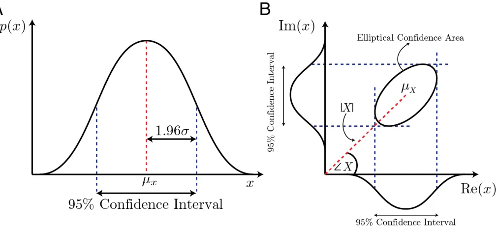
When considering the uncertainty associated with a real val-ued measurement of a system it is very common to assume that the variable is drawn from a normal probability distribution [23]. The assumption of normality allows the distribution to be defined by the statistics of the normal distribution, the meanµ
and the varianceσ2. The uncertainty can then be displayed by
a percentage confidence interval which defines the interval in which the measurement falls within a percentage probability, see Figure 1A.
When the measurement is drawn from a bivariate normal distribution the statistics are defined by the vector mean µ
and covariance given by
Σ =
σ1,1 σ1,2
σ2,1 σ2,2
(11)
where σ1,1, σ2,2 are the variance in the 1st and 2nd variate
respectively and σ1,2 = σ2,1 is the covariance between the
two. The mean and covariance matrix define a probability distribution in the space of two variates that characterise the uncertainty. Analogous to the univariate measurement where the uncertainty can be displayed as a confidence interval, for the bivariate measurement a percentage confidence area is defined by the uncertainty in each variate and the correlation between them [24]. In the space of the two variates the confidence area is elliptical.
A complex valued variable is often represented in two parts, real and imaginary (commonly plotted on an Argand diagram), where
x=a+jb= Re(x) +jIm(x). (12) Complex variables can hence be though of as bivariate:
X = [Re(x),Im(x)]. (13) In general the variance in the real and imaginary parts of the measurement will not be independent and can therefore be assumed to be drawn from the bivariate normal distribution
X ∼ N
X|
µRe(x)
µIm(x)
,ΣRe(x),Im(x)
. (14)
The uncertainty in a complex variable is then displayed as an elliptical confidence area in the real-imaginary space, see Figure 1B. Another alternative representation for complex variables is in gain-phase form, this is common practice when considering systems in the frequency domain [1]. The gain-phase representation of a complex variable can also be considered as bivariate and so can be treated similarly. Care should be taken when using the gain-phase representation however because the uncertainty predictions at near zero gain can be inaccurate in some cases, see [13].
E. Classical uncertainty propagation
Propagation of uncertainty is the calculation of the un-certainty associated with the output of some function by considering the uncertainty in its input variables and how these
propagatethrough the equation. A discussion of the classical treatment of uncertainty propagation follows.
Firstly consider a functionf which is a linear combination of p variables x1, x2, . . . , xp with coefficients c1, c2, . . . , cp,
such that
y=f(x1, x2, . . . , xp) = p X
i=1
cixi=cx (15)
where the uncertainty associated with the input variables is described by the covariance matrix
Σx=
σ2x1 σx1,2 · · · σx1,p
σx2,1 σ
2
x2 · · · σx2,p
..
. ... . .. ...
σxp,1 σxp,2 · · · σ
2
xp
Fig. 1. The uncertainty in a complex variable can be represented by a bivariate normal distribution creating an elliptical uncertainty area in the real imaginary space. A) The probability distribution of a real valued univariate variable with its 95% confidence intervals. B) The elliptical confidence area of a complex variable represented by a bivariate normal distribution.
The variance of the output variable,y, is then given by [11]
σ2y= p X
i p X
j
ciΣxijcj (17)
In the general case f is allowed to take the form of some non-linear combination of x1, x2, . . . , xp and a linearisation
of f has to be performed (except in some special cases where the variance can be calculated exactly, see for example [25]). The classical propagation law is found by approximatingf by a first order Taylor expansion
y≈f0+
p X
i=1
∂f ∂xi
xi (18)
which is valid only when the uncertainties associated with the input variables are small enough so that they satisfy the local linear approximation.
The variance of the non-linear function f(x1, x2, . . . , xp)
can be found from Equation (17) with
ci=
∂f ∂xi
(19)
producing the classical law of uncertainty propagation
σy2= n X
i=1
n X
i=1
∂f ∂xi
Σx
i,j
∂f ∂xj
. (20)
This method is used extensively for calculating errors in scientific measurements as recommended in the Guide to the Expression of Uncertainty in Measurement [11].
F. Multivariate uncertainty propagation
As shall be seen in Section II-G, when the output variable is complex valued it is necessary to consider a multivariate
form of the propagation law. The multivariate method allows for the estimation of uncertainty for multiple output variables simultaneously as well as the correlations between them.
The functionf considered in the previous section is modi-fied so that it is now a vector function denotedf of lengthq
with a real valued vector output,y, such that
y=f(x) =hf1(x), f2(x), . . . , fq(x)i (21)
The multivariate uncertainty propagation equation is then given by [13], [15], [26]
Σy=JΣxJT (22)
whereΣyis the covariance matrix for the output vectoryand
Jis the Jacobian matrix given by
J=
∂f1 ∂x1
∂f1 ∂x2 · · ·
∂f1 ∂xp
∂f2 ∂x1
∂f2 ∂x2 · · ·
∂f2 ∂xp
..
. ... . .. ...
∂fq
∂x1 ∂fq
∂x2 · · · ∂fq
∂xp
(23)
Note that for a scalar output, Equation (22) reduces to the classical case given by (20). It is worth noting the similarity to the propagation step in the extended Kalman filter (EKF), which makes the same assumption that higher order terms in the Taylor series are negligible, based on the approximation of local linearity.
G. Propagation of uncertainty in complex valued variables
the input and output variables of the function are complex valued. Here the input variables will be the real valued parameters of a time-domain, input-output model and only the output variable will be complex valued. The discussion presented here is based on the referenced work but considering a complex valued output only.
The complex valued output to some vector function f can be represented as the vector y = [y1, y2], where y1 and y2
represent the real and imaginary components of the output, such that
y=hf1(x), f2(x)i (24)
where the functions f1(x)andf2(x)map the input vector x
into the real and imaginary part of the output respectively. The variance propagation equation is hence given by (22) whereJis a[2×p]Jacobian matrix given by
J=
"∂f 1 ∂x1
∂f1 ∂x2 · · ·
∂f1 ∂xp
∂f2 ∂x1
∂f2 ∂x2 · · ·
∂f2 ∂xp
#
(25)
The covariance matrix representing the uncertainty associ-ated with the input variables remains unchanged (i.e.is given by equation (16)).
This method therefore allows uncertainty to be approxi-mately propagated through a function of multiple input vari-ables into a complex output. It is now in the correct form to approximate the uncertainty in the complex valued FRF as a function of uncertain model parameters. The approach is adopted in the following section.
III. FREQUENCY RESPONSE UNCERTAINTY PROPAGATION FOR GENERAL INPUT-OUTPUT MODELS
In this section, variance propagation from a time-domain nonlinear system into the (complex-valued) frequency-domain is derived for the GFRF, the NOFRF and nth
-order output spectra. In addition, an algorithm for the complete model-based analysis of nonlinear systems is presented, from sys-tem identification in the time-domain, to generation of the frequency response functions and the associated uncertainty propagation novel to this paper.
A. Uncertainty propagation into the GFRF, NOFRF and nth
-order output spectra
The GFRF is a complex valued function, typically visualised in the space of the magnitude and phase. It is therefore desirable to propagate the parameter uncertainty, characterised by Σθ, directly into the bi-variate magnitude-phase space rather than the real-imaginary space given by (13). Employing the multivariate propagation law, given by (22), the covariance in the magnitude and phase of the GFRF,Hn(jω1, . . . , jωn),
is given by
Σ|Hn|,∠Hn=JH(ω,θ)ΣθJH(ω,θ)
T, (26)
where
JH(ω,θ) = "∂|H
n|
∂θ1
∂|Hn|
∂θ2 . . . ∂|Hn|
∂θM
∂∠Hn
∂θ1
∂∠Hn
∂θ2 . . . ∂∠Hn
∂θM
#
(27)
where the GFRF covariance matrix is a function of the model parameters θ and the frequencies ω1, . . . , ωn. In order to
evaluate (27), expressions for the partial differentials of the magnitude and phase with respect to the model parameters must be derived, which is performed in the next section.
Multivariate uncertainty propagation for the NOFRFs,
Gn(jω), can be similarly described as
Σ|Gn|,∠Gn =JG(ω,θ)ΣθJG(ω,θ)
T, (28)
where
JG(ω,θ) = "∂|G
n|
∂θ1
∂|Gn|
∂θ2 . . . ∂|Gn|
∂θM
∂∠Gn
∂θ1
∂∠Gn
∂θ2 . . . ∂∠Gn
∂θM
#
. (29)
and also noting that for arbitrarym
∂Gn ∂θm = R∞ −∞. . . R∞ −∞
∂Hn(jω1,...,jωn)
∂θm
Qn
i=1U(jωi)dω1. . .dωn R∞
−∞. . .
R∞
−∞
Qn
i=1U(jωi)dω1. . .dωn
(30)
Multivariate uncertainty propagation for thenth-order output
spectra,Yn(jω), can also be described as
Σ|Yn|,∠Yn=JY(ω,θ)ΣθJY(ω,θ)
T,
(31)
where
JY(ω,θ) = "∂|Y
n|
∂θ1
∂|Yn|
∂θ2 . . . ∂|Yn|
∂θM
∂∠Yn
∂θ1
∂∠Yn
∂θ2 . . . ∂∠Yn
∂θM
#
(32)
and also noting that
∂Yn
∂θm
= n
−1/2
(2π)n−1
Z
ω
∂Hn(jω1, . . . , jωn)
∂θm
n Y
i=1
U(jωi)dσnω.
(33)
B. Partial derivatives of magnitude and phase with respect to model parameters
The multivariate uncertainty propagation expressions for GFRFs, NOFRFs and the nth-order output spectra all require
the definition of the partial derivative of the magnitude and phase with respect to themth model parameter. Therefore, to
avoid repetition we consider solving this problem for a general complex valued function, F, assuming we require ∂|Fn|
∂θm and
∂∠Fn
∂θm , for m= 1, . . . , M.
1) Partial derivative of the magnitude: firstly, noting that
Re(F) = 1
2(F+F), Im(F) = 1
whereF represents the complex conjugate ofF, and the partial derivative can be found by
∂|F| ∂θm
= ∂
∂θm
(F F)12
= ∂
∂F(F F)
1 2 ∂F
∂θm
+ ∂
∂F(F F)
1 2 ∂F
∂θm
=1 2F(F F)
−1 2 ∂F
∂θm
+1 2F(F F)
−1 2 ∂F
∂θm
= 1 2|F|
F ∂F ∂θm
+F ∂F ∂θm
= 1
|F|Re
F ∂F ∂θm
. (35)
2) Partial derivative of the phase: Taking the derivative of the angle ofF
∂∠F ∂θm =
∂
∂X arctan(X) ∂X ∂θm
, (36)
whereX =Im(Re(FF)). The derivative ofX is given by
∂X ∂θm
= ∂
∂Im(F)
Im(F) Re(F)
∂Im(F)
∂θm
+ ∂
∂Re(F)
Im(F) Re(F)
∂Re(F)
∂θm
= 1 Re(F)
∂Im(F)
∂θm
− Im(F)
Re(F)2
∂Re(F)
∂θm
.
(37)
Employing equation (34) in Equation (37) leads to,
∂X ∂θm = 1 j ∂F ∂θm − ∂F ∂θm
F+F
(F+F)2 −1 j ∂F ∂θm + ∂F ∂θm
F−F
(F+F)2
(38)
where the term on the left hand side has been multiplied by a factor ofF+F in the numerator and denominator. Collecting terms
∂X ∂θm
= 2
j(F+F)2
F ∂F ∂θm
−F ∂F ∂θm
= 4 (F+F)2Im
F ∂F ∂θm
= 1 Re(F)2Im
F ∂F ∂θm
. (39)
The derivative ofarctan(X)is given by the identity
∂
∂Xarctan(X) =
1 1 +X2 =
Re(F)2
|F|2 . (40)
The general solution is then found by substituting equations (39) and (40) into Equation (36) such that,
∂∠F ∂θm
= 1
|F|2Im
F ∂F ∂θm
. (41)
C. Algorithm for frequency-domain uncertainty analysis of nonlinear systems
The frequency-domain uncertainty analysis for a nonlinear system can be performed using the following algorithm, which describes the full procedure, from standard steps of nonlinear system identification through to the novel frequency-domain uncertainty analysis derived in this paper.
The first step is to identify a time-domain nonlinear model of the system, if one is not already available,
1) (Optional) Time-domain identification of a nonlinear model of the system. The identified model must include an estimate of both the parameter means θµ and the
parameter covariance Σθ.
Any suitable method can be used, e.g. for input design see [27], for identification algorithms see [20], [28]–[30] and for correlation-based validation methods see [31], [32].
The initial frequency-domain analysis can be performed using the identified model along with the following steps,
2) Calculate GFRFs, Hn, for n = 1, . . . , N using (7),
where the procedure makes use of the time-domain model obtained in step 1, e.g as described in [3] or using an efficient algorithm as described in [22].
3) Calculate thenth-order input spectra using (10) forn=
1, . . . , N. 4) Calculate the nth
-order NOFRFs, for n = 1, . . . , N, analytically using (9) or the data-driven algorithm in [4]. 5) Filter the nth
-order input spectra with the nth
-order NOFRF to obtain the nth
-order output spectra as de-scribed in (8).
Finally, the frequency-domain uncertainty analysis novel to this paper can be implemented by the following steps,
6) Calculate the partial derivatives of the GFRF with re-spect to the model parameters ∂Hn
∂θm using the definition
of Hn obtained in step 2.
7) Define F = [F1, . . . , FN], where Fn is the nth-order
frequency domain description of interest, Hn, Gn, or
Yn.
8) Calculate the partial derivatives in gain, ∂|Fn|
∂θm , and
phase, ∂∠Fn
∂θm , using (35) and (41) respectively.
9) DefineJF(ω,θ)using (27), (29) or (32) respectively.
10) Calculate the uncertainty in gain and phase Σ|Fn|,∠Fn,
forn= 1, . . . , Nmusing (26), (28) or (31) respectively.
IV. NUMERICAL EXAMPLES
A. Nonlinear model uncertainty propagation for a simulated system
We demonstrate the procedure for propagating uncertainty into the frequency response for nonlinear systems using the following NARX model,
yk =θ1yk−1+θ2yk−2+θ3uk−1
+θ4uk−2+θ5u2k−1+θ6yk2−1+ek (42)
The first order GFRF is given by
H1(ω,θ) =
θ3e−jω+θ4e−2jω
1−θ1e−jω−θ2e−2jω
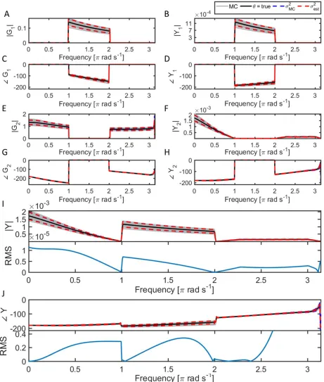
Fig. 2. Comparison of frequency-domain uncertainty estimates generated by Monte Carlo sampling and uncertainty propagation for a simulated nonlinear system. True parameter values (Black), Monte Carlo samples (Grey), sampled variance (Blue dashed - note that the Red dashed line overlays the Blue dashed line in most instances) and propagated variance (Red dashed). A) Magnitude ofG1, B) Magnitude ofY1, C) Phase ofG1, D) Phase ofY1, E) Magnitude of G2, F) Magnitude ofY2, G) Phase ofG2, H) Phase ofY2, I) Top: Magnitude ofY. Bottom: RMS error between estimated variance and propogated variance , and J) Top: Phase ofY. Bottom: RMS error between estimated variance and propogated variance.
The second order GFRF is given by
H2(ω1, ω2) =
θ5e−jπ(ω1+ω2)+θ6H1(ω1)H1(ω2)e−jπ(ω1+ω2)
1−θ1e−j(ω1+ω2)−θ2e−2j(ω1+ω2) (44)
Note that in general H1(ω) cannot be a function of the
parameters associated with higher order terms, in this case
θ5 and θ6. However, higher order GFRFs may depend on
lower order terms. Similarly, the partial derivatives of the
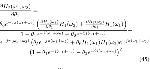
partial derivatives. For example, differentiating H2(ω1, ω2)
with respect to θ1 gives
∂H2(ω1, ω2)
∂θ1 =
θ6e−jπ(ω1+ω2)
∂H 1(ω1)
∂θ1 H1(ω2) +
∂H1(ω2) ∂θ1 H1(ω1)
1−θ1e−j(ω1+ω2)−θ2e−2j(ω1+ω2) +
e−jπ(ω1+ω2) θ5e−jπ(ω1+ω2)+θ6H1(ω1)H1(ω2)e−jπ(ω1+ω2)
1−θ1e−j(ω1+ω2)−θ2e−2i(ω1+ω2)
2
(45)
which is dependent on ∂H1(ω)
∂θ1 . Although the differentiation is
simple to perform it indicates that, in general, it is necessary to evaluate the differentials of all lower order FRFs.
To demonstrate the frequency-domain analysis procedure, the full algorithm given in section III.C was implemented here, beginning with identification of the model from simulated data. The system described by the nonlinear model in (42) was simulated for N = 1000 samples in response to an input excitation signal uk drawn from a uniform distribution
in the range [−0.5,0.5]. The parameters were defined as
θ = (0.2,0.1,0.1,0.05,0.2,0.5)T and ek was defined as an
i.i.d white noise sequence drawn from the normal distribution
ek ∼ N(0, σ2e)whereσe2= 0.0005.
Model parameters were estimated using an algorithm based on variational Bayesian inference, which intrinsically gener-ates parameter uncertainty [20]. The resulting posterior distri-bution for the parameters was normally distributed with mean and covariance given by
µθ=
0.189 0.108 0.099 0.049 0.198 0.627T Σθ= 10−1×
0.025 −0.008 0.000 −0.002 −0.000 −0.122
−0.008 0.010 −0.000 0.001 −0.000 0.001 0.000 −0.000 0.002 −0.000 −0.000 0.000
−0.002 0.001 −0.000 0.000 0.000 0.000
−0.000 −0.000 −0.000 0.000 0.001 −0.010
−0.122 0.001 0.000 0.000 −0.010 1.586
In this example, only the NOFRF and the output spectra were analysed. This is because the first order GFRF contains similar information to the first order NOFRF and so is re-dundant, whilst the second order GFRF is 2-dimensional and is therefore difficult to analyse, whilst higher order GFRFs cannot be visualised at all. In the general case, it would appear simpler to take this approach and focus on the NOFRF, which also has the advantage of being input-specific. Also, note that we only analyse the magnitude (or gain) of the nonlinear sys-tem here, which is most interesting for checking phenomena such as resonances, super/sub-harmomics and energy transfer across frequencies.
The covariance in the NARX model parameters was prop-agated into the nth
-order NOFRF and the nth
-order output spectra using (28)-(29) and (31)-(32) respectively. The input signal used to evaluate the NOFRF was uniform across fre-quencies in the band [1,2] rad s−1 and zero elsewhere, see [4] for the generation of such a signal. Monte Carlo sampling
was used as a comparison to benchmark and validate the approach for uncertainty propagation, using NM C = 100
samples (the number of samples was relatively small because the computational cost of repeatedly performing the frequency-domain mapping is prohibitively expensive). The evaluation of the NOFRFs for the true parameter vector took 0.89 seconds with a further 0.068 seconds to propagate the uncertainty with timings averaged over 100 runs. The evaluation of NOFRFs for
NM C = 100 samples took 88.7 seconds. Computations were
performed on a laptop computer with an intel(r) core(tm) i7 CPU @ 2.GHz processor and 8GB RAM.
The propagated variance in the gain and phase of both the NOFRF and the nth-order output spectra showed good
agreement to the sampled variance in all cases, see Figure 2A-H. The output spectrum was approximated as Y ≈Y1+Y2,
assuming higher orders have a negligible contribution to the output. The variance in the gain and phase of the output spectrum was calculated as σ2
Y = σ2Y1 +σ2Y2 and similarly
shows good agreement to the sampled variance, see Figure 2I-J. The error between the propogated variance and the MC sampled variance on both the gain and phase is shown in Figure (2) I and J respectively, where the error is expressed as the root mean square error. Errors are only shown forY, given that the first and second order frequency spectra are located at exclusive frequency bands, the errors of the individual orders can be inferred. Normalised errors are identical for Gi and
Yi, this is explained by noting that the source of error in both
Equations (30) and (33) originate from Hi. RMS errors are
small in both gain and phase for low frequencies, large errors are observed in the phase at high frequencies (>2.5 rad s−1).
B. Nonlinear model uncertainty propagation for a real-world experimental system
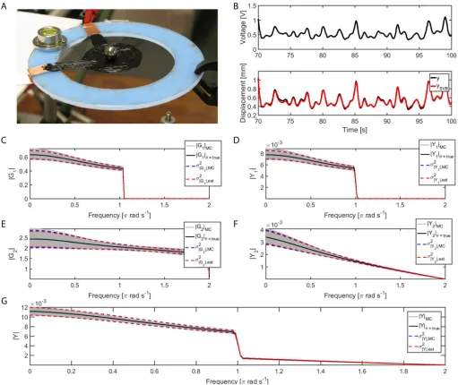
In this section the uncertainty propagation method is applied to characterising the frequency domain uncertainty of a class of soft-smart actuator known as a dielectric elastomer actuator (DEA), a type of electroactive polymer used in robotics that is known to display nonlinear behaviour [33]. Due to the wide fabrication tolerances of DEA uncertainty characterisation is particularly pertinent. The experimental set up and data collection procedure has been described before [34], therefore only a brief description is given here to put the case study into context.
[image:9.612.51.301.80.196.2]Fig. 3. Comparison of frequency-domain uncertainty estimates generated by Monte Carlo sampling and uncertainty propagation for identified nonlinear models of two dielectric elastomer actuators (DEAs). A) Picture of the DEA experimental set-up. B) Top: DEA system input (Voltage). Bottom: measured DEA system output (Displacement) DEA system (Black) with the model predicted output of the model identified with the SVB-NARX algorithm (Red). C-G) True parameter values (Black) with the Monte Carlo samples (Grey), sampled variance (Blue dashed - note that the Red dashed line overlays the Blue dashed line in most instances) and propagated variance (Red dashed) for experiment 1. C) Magnitude ofG1, D) Magnitude ofY1, E) Magnitude ofG2,F) Magnitude of Y2and G) Magnitude ofY.
The DEA nonlinear model was identified using the sparse variational Bayes-NARX (SVB-NARX) algorithm described in [20], which produced a model with accurate predictive capability, see Figure 3B. First and second order GFRFs, NOFRFs and output spectra were calculated for the DEA using the identified model, along with the variance using uncertainty propagation proposed here. Monte Carlo sampling was also used to generate numerical estimates of the variance for a comparison to uncertainty propagation. The propagated variance in the NOFRFs and output spectra closely matched the variance in the gain of the sampled output spectra, see Figure 3C-G.
The close agreement between the uncertainty propagation method and Monte Carlo sampling demonstrates the
effec-tiveness of uncertainty propagation, which avoids the compu-tational cost of sampling. Uncertainty propagation, therefore, provides a valuable addition to methods used in the analysis of nonlinear systems.
V. SUMMARY
Monte Carlo sampling from the model parameter distribution in order to build up a posterior distribution in the frequency-domain. A key advantage of the uncertainty propagation method is that it avoids the repeated sampling involved in Monte Carlo simulations and the associated computational cost. Uncertainty propagation is therefore a useful and im-portant addition to the suite of tools used in the analysis of nonlinear systems.
APPENDIX A. Direct evaluation of NOFRFs
This section describes the direct evaluation of NOFRFs from time-domain model simulations (as opposed to their indirect evaluation via GFRFs) using the method defined in [4].
Firstly, note that the output spectra of a nonlinear system as defined in (8) can be re-written as a function of the NOFRFs in the following form,
Y(jω) =
N X
n=1
Yn(jω) = N X
n=1
Gn(jω)Un(jω)
=
N X
n=1
Gn(jω)αnUn∗(jω)
(46)
where Gn(jω) is the nth-order NOFRF, and the input
fre-quency spectra of a specific time-domain inputu(t) =αu∗(t) is defined as
Un(jω) =
n−1/2
2πn−1
Z ∞
−∞
. . .
Z ∞
−∞
n Y
i=1
U(jωi)dω1. . .dωn
=αnn
−1/2
2πn−1
Z ∞
−∞
. . .
Z ∞
−∞
n Y
i=1
U∗(jωi)dω1. . .dωn
=αnUn∗(jω)
(47)
whereU∗(jω)is the Fourier transform ofu∗(t)and
Un∗(jω) =
n−1/2
2πn−1
Z ∞
−∞
. . .
Z ∞
−∞
n Y
i=1
U∗(jωi)dω1. . .dωn
(48) The key idea for estimating the NOFRFs is to define a rep-resentation of (46) based on numerical samples of frequency-domain transformations of time-frequency-domain input-output data, generated from K time-domain model simulations, where
K ≥N. TheK model simulations each use a distinct input signal, αiu∗(t), for i= 1, . . . , K, where a single waveform,
u∗(t), is scaled by increasing amplitudes defined byαi, where
αK > αK−1> . . . > α1>0, leading to
Y=UG (49)
where
Y= [Y1∗(jω), . . . , YK∗(jω)]T (50)
U=
α1U1∗(jω) . . . αN1 UN∗(jω)
..
. ...
αKU1∗(jω) . . . αNKUN∗(jω)
(51)
G= [G1(jω), . . . , GN(jω)]T (52)
where Yi∗(jω) for i = 1, . . . , K is the frequency-domain transformation of the corresponding time-domain output signal from the model simulation, yi∗(t) for i = 1, . . . , K, which can be obtained in practice by taking the fast Fourier trans-form (FFT) of yi∗(t). Note also that the terms Ui∗(jω), for
i= 1, . . . , K, can be obtained in practice by taking the FFT of (u∗(t))i, fori= 1, . . . , K.
Given Y and U it is straightforward to estimate the NOFRFs in closed form via
ˆ
G= UHU−1
UHY (53)
whereUH
denotes the conjugate transpose ofU.
Once the NOFRFs have been estimated, thenth-order output
spectra can also be reconstructed as
Yn(jω) = ˆGn(jω)Un(jω)for n= 1, . . . , N (54)
where Gˆn is an element of Gˆ and Un(jω) is the FFT of
(u(t))n, for n= 1, . . . , N.
REFERENCES
[1] L. Ljung,System identification: theory for the user, 2nd ed., ser. Prentice Hall information and system sciences series. Upper Saddle River, NJ: Prentice Hall PTR, 1999.
[2] S. A. Billings,Nonlinear system identification: NARMAX methods in the time, frequency, and spatio-temporal domains. Wiley, 2013. [3] S. A. Billings and K. M. Tsang, “Spectral analysis for non-linear
systems, Part I: Parametric non-linear spectral analysis,” Mechanical Systems and Signal Processing, vol. 3, no. 4, pp. 319–339, 1989. [4] Z. Q. Lang and S. A. Billings, “Energy transfer properties of non-linear
systems in the frequency domain,” International Journal of Control, vol. 78, no. 5, pp. 345–362, Mar. 2005.
[5] H. Zhang and S. Billings, “Analysing non-linear systems in the fre-quency domain–I. the transfer function,”Mechanical Systems and Signal Processing, vol. 7, no. 6, pp. 531–550, 1993.
[6] Z. Peng, Z.-Q. Lang, and S. Billings, “Resonances and resonant frequen-cies for a class of nonlinear systems,”Journal of Sound and Vibration, vol. 300, no. 3, pp. 993–1014, 2007.
[7] G. C. Goodwin, M. Gevers, and B. Ninness, “Quantifying the error in estimated transfer functions with application to model order selection,”
IEEE Transactions on Automatic Control, vol. 37, no. 7, pp. 913–928, 1992.
[8] B. Wahlberg and L. Ljung, “Hard frequency-domain model error bounds from least-squares like identification techniques,”IEEE Transactions on Automatic Control, vol. 37, no. 7, pp. 900–912, 1992.
[9] X. Bombois, B. Anderson, and M. Gevers, “Frequency domain image of a set of linearly parametrized transfer functions,” inEuropean Control Conference (ECC), 2001, pp. 1416–1421.
[10] K. Worden, “Confidence bounds for frequency response functions from time series models.”Mechanical Systems and Signal Processing, vol. 12, no. 4, pp. 559–569, Jul. 1998.
[11] Bureau International des Poids et Mesures,Guide to the Expression of Uncertainty in Measurement. International Organization for Standard-ization, 1995.
[12] R. Pintelon and J. Schoukens, “Measurement of frequency response functions using periodic excitations, corrupted by correlated input/output errors,” IEEE Transactions on Instrumentation and Measurement, vol. 50, no. 6, pp. 1753–1760, 2001.
[13] N. M. Ridler and M. J. Salter, “An approach to the treatment of uncertainty in complex S-parameter measurements,”Metrologia, vol. 39, no. 3, p. 295, 2002.
[14] B. D. Hall, “Calculating measurement uncertainty for complex-valued quantities,”Measurement Science and Technology, vol. 14, no. 3, p. 368, 2003.
[15] ——, “On the propagation of uncertainty in complex-valued quantities,”
Metrologia, vol. 41, no. 3, pp. 173–177, Jun. 2004.
[17] Thomas E. Fricker, J. E. Oakley, N. D. Sims, and K. Worden, “Proba-bilistic uncertainty analysis of an FRF of a structure using a Gaussian process emulator,”Mechanical Systems and Signal Processing, vol. 25, no. 8, pp. 2962–2975, 2011.
[18] O. Nelles,Nonlinear System Identification. Berlin: Springer, 2001. [19] J. Sj¨oberg, Q. Zhang, L. Ljung, A. Benveniste, B. Delyon, P.-Y.
Gloren-nec, H. Hjalmarsson, and A. Juditsky, “Nonlinear black-box modeling in system identification: a unified overview,”Automatica, vol. 31, no. 12, pp. 1691–1724, 1995.
[20] W. R. Jacobs, T. Baldacchino, T. J. Dodd, and S. R. Anderson, “Sparse bayesian nonlinear system identification using variational inference,”
IEEE Transactions on Automatic Control, 2018.
[21] T. Baldacchino, S. R. Anderson, and V. Kadirkamanathan, “Structure detection and parameter estimation for NARX models in a unified EM framework,”Automatica, vol. 48, no. 5, pp. 857–865, May 2012. [22] J. P. Jones and K. Choudhary, “Efficient computation of higher order
frequency response functions for nonlinear systems with, and without, a constant term,”International Journal of Control, vol. 85, no. 5, pp. 578–593, May 2012.
[23] A. Lyon, “Why are normal distributions normal?”The British Journal for the Philosophy of Science, vol. 65, no. 3, pp. 621–649, 2014. [24] W. K. H¨ardle and L. Simar, Applied Multivariate Statistical Analysis.
Berlin, Heidelberg: Springer Berlin Heidelberg, 2012.
[25] L. A. Goodman, “On the Exact Variance of Products,”Journal of the American Statistical Association, vol. 55, no. 292, p. 708, Dec. 1960. [26] R. Willink and B. D. Hall, “A classical method for uncertainty analysis
with multidimensional data,”Metrologia, vol. 39, no. 4, p. 361, 2002. [27] I. Leontaritis and S. Billings, “Experimental design and identifiability for
non-linear systems,”International Journal of Systems Science, vol. 18, no. 1, pp. 189–202, 1987.
[28] S. Chen, S. A. Billings, and W. Luo, “Orthogonal least squares methods and their application to non-linear system identification,”International Journal of Control, vol. 50, no. 5, pp. 1873–1896, Nov. 1989. [29] L. Piroddi and W. Spinelli, “An identification algorithm for polynomial
NARX models based on simulation error minimization,”International Journal of Control, vol. 76, no. 17, pp. 1767–1781, Nov. 2003. [30] T. Baldacchino, S. R. Anderson, and V. Kadirkamanathan,
“Com-putational system identification for Bayesian NARMAX modelling,”
Automatica, vol. 49, no. 9, pp. 2641–2651, Sep. 2013.
[31] S. A. Billings and W. S. F. Voon, “Correlation based model validity tests for non-linear models,”International Journal of Control, vol. 44, no. 1, pp. 235–244, Jul. 1986.
[32] S. Billings and Q. Zhu, “Nonlinear model validation using correlation tests,”International Journal of Control, vol. 60, no. 6, pp. 1107–1120, 1994.
[33] Y. Bar-Cohen, Ed.,Electroactive polymer (EAP) actuators as artificial muscles: reality, potential, and challenges, 2nd ed. Bellingham, Wash: SPIE Press, 2004.
[34] W. R. Jacobs, E. D. Wilson, T. Assaf, J. Rossiter, T. J. Dodd, J. Porrill, and S. R. Anderson, “Control-focused, nonlinear and time-varying modelling of dielectric elastomer actuators with frequency response analysis,”Smart Materials and Structures, vol. 24, no. 5, p. 055002, May 2015.
William R. Jacobs received the M.Phys. degree in physics with mathematics from the University of Sheffield, Sheffield, UK, in 2010 and the Ph.D. degree in nonlinear system identification from the University of Sheffield in 2016.
He is currently working as a Research Associate in the Rolls Royce University Technology Centre, Department of Automatic Control and Systems En-gineering at the University of Sheffield.
Tony Dodd received the B.Eng. degree in aerospace systems engineering from the University of Southampton, Southampton, UK, in 1994 and the Ph.D. degree in machine learning from the Department of Electronics and Computer Science, University of Southampton in 2000.
From 2002 to 2010, he was a Lecturer in the Department of Automatic Control and Systems En-gineering at the University of Sheffield, Sheffield, UK, and from 2010 to 2015 was a Senior Lecturer at the University of Sheffield. He is currently a Professor of Autonomous Systems Engineering and Director of the MEng Engineering degree programme at the University of Sheffield.
Sean R. Andersonreceived the M.Eng. degree in control systems engineering from the Department of Automatic Control and Systems Engineering, Uni-versity of Sheffield, Sheffield, UK, in 2001 and the Ph.D. degree in nonlinear system identification and predictive control from the University of Sheffield in 2005.